Indirect Vector Control of Linear Induction Motors Using Space Vector Pulse Width Modulation

1  Introduction

Induction machines are being used in many modern applications as these machines have features of simple assembly, low moment of inertia, and high initial torque with low ripple factor. These induction motors are used in heavy-duty applications by developing different control schemes [1]. The most important application of the LIM is the traction system, as the use of LIM in the traction system facilitated the technical design by direct drive [2]. A direct drive system requires an electric motor with high torque in a specified space. LIM in a proper shape and provided with variable frequency meets the required performance features by a driving system in electric traction. For many modern and heavy-duty applications such as mechanical manufacturing, robotics, CNC machines, and traction systems, linear motors are considered a better choice than rotary machines as they offer superior output and efficiency in modern applications [3–7]. The working principle of a linear motor is simple: the magnetic flux of the moving part is synchronized with the stationary section, which converts electromagnetic energy to linear motion, and the load is directly fixed with the mover. The invention of linear machines eliminated many tools such as ball and screw, belt and pulley, and other turning arrangements which were used for the conversion of rotary motion to linear motion, as well as losses involved in this conversion process [8–11]. Additionally, linear machines provide speed precision with improved efficiency and are easy to construct as the idea is simple: cut the rotary motor radially and set it flat. The working rule for linear and rotary induction motors is the same, but the air gap is more extensive in LIM, and the mover is shorter for a track, resulting in end effects [12].

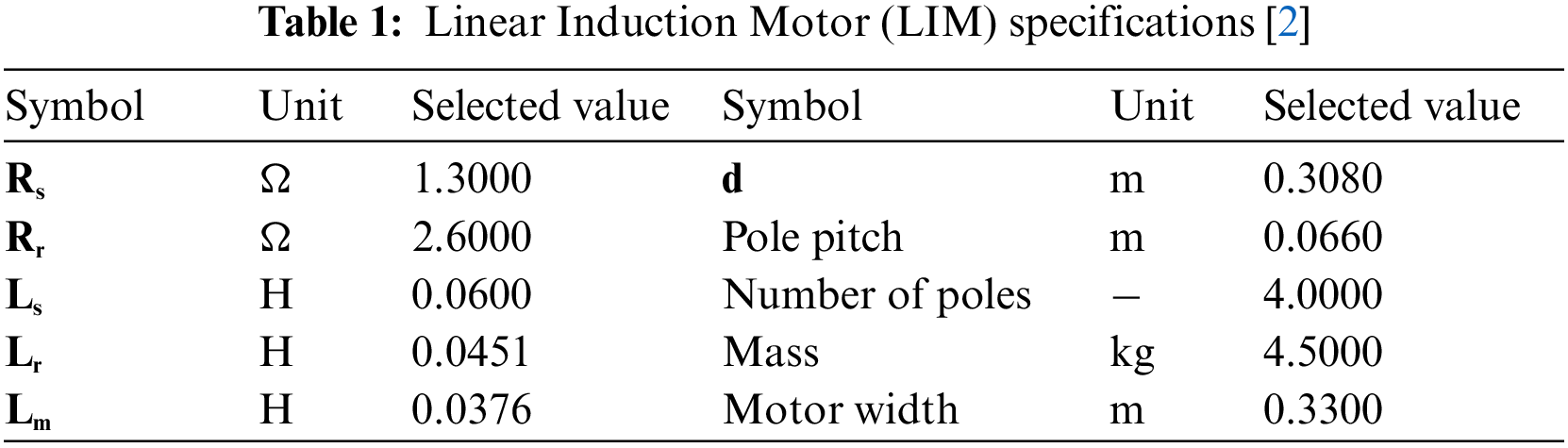
The dynamic performance, precise speed control, and trust force are significant, especially for heavy-duty applications. This research aims to develop SVPWM based control scheme, considering end effects, for speed and thrust force control of LIM, which will be applicable for a different speed range of low to high-speed applications. For this purpose, LIM’s working principle and construction are explored in depth. The dynamic model is developed in MATLAB Simulink after performing detailed mathematical modeling. Regarding the LIM, one of the objectives of research work is to establish the electrical parameters of the LIM to predict the response of dynamics associated with this system. LIM description in the dynamic response requires interaction between electrical and mechanical subsystems. For this purpose, governing differential equations representing the different phenomena of the electromechanical system is considered. A reliable simulation model is developed that describes the LIM dynamics derived from mathematical modeling, and for this purpose, the specifications of the LIM are chosen based on the previous study [2,13]. Relevant parameters are attached in Annexure, and motor specifications considered in this research are presented in Table 1. A valid SVPWM-based control scheme is implemented, and an optimized set of parameters are achieved in MATLAB Simulink.

Based on the developed dynamic model and integrated SVPWM inverter, the next step to control the electromechanical system is designing and tuning the PI controller. The proposed scheme contains three parts, a dynamic model of LIM, an SVPWM modulator-based inverter, and the PI controllers. Precise control of LIM parameters, including speed and thrust force, is given, verified by the simulation results.

2  Electromechanical Dynamic Modeling of Linear Induction Motor

In most applications related to control machine drives, transient response analysis of the electrical machines is critical, and a dynamic d-q model is developed for this purpose [14]. The d-q model of the equivalent electrical circuit, considering end effects, is used to present the dynamics for LIM and complete steps to develop the dynamic model are represented in Fig. 1 [15].

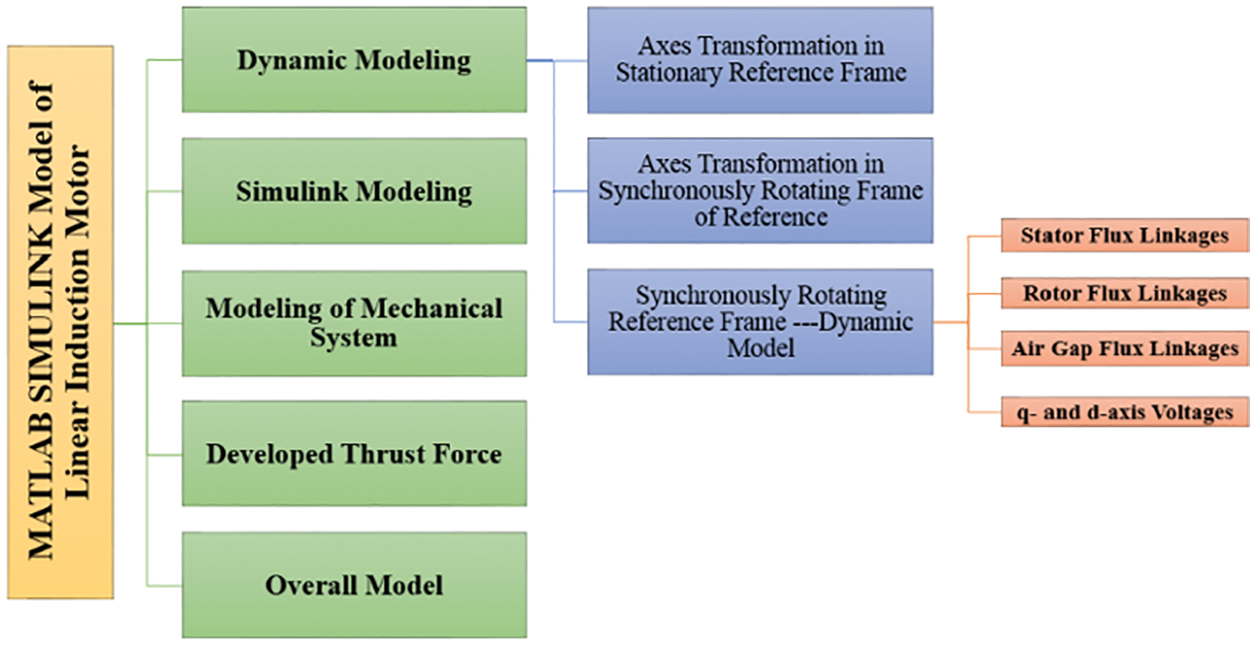
Figure 1: Electromechanical dynamic modeling steps for linear induction motor [15]

In the dynamic model, q-axis equivalent circuit for LIM is the same as of the rotary induction machine (RIM), and the reason for this similarity is that the parameters are independent of the end effects. For the d-axis equivalent circuit of LIM, end effects are reflected in the equivalent circuit of RIM. So, the development of an appropriate dynamic model of LIM needs consideration of fluxes induced due to moving parts named as end effect. The end effect at the starting and ending points from the secondary is reflected as a factor f(Q), mathematically given as in Eq. (1):

f(Q)=1−1−e−QQ(1)

The value of Q in (1) is given in Eq. (2):

Q=dTr.v=d (LrRr).v=dRr(Lm+Lir).v(2)

where Rr represents resistance and Lr indicates the inductance of the rotor, respectively, d gives the length of primary in meters, v shows the linear speed of the primary in m/s [16].

For dynamic modeling, 3-φ stationary frame of reference (as-bs-cs) variables are changed to 2-φ stationary frame of reference (ds-qs) variables, and after that, 2-φ variables of stationary frame of reference are changed to synchronously rotating frame of reference [17].

After considering end effects, the first step for dynamic modeling is the transformation of axes a-b-c in the ds-qs stationary frame of reference, as explained in Fig. 2, and the conversion matrix for this transformation is represented in Eq. (3):

[vsqsvsdsvsos]=[cos⁡θsin⁡θ1cos⁡(θ−2π3)sin⁡(θ−2π3)1cos⁡(θ+2π3)sin⁡(θ+2π3)1][vasvbsvcs](3)

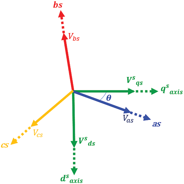
Figure 2: Stationary frame (abc-dq) transformation

Synchronously rotating axes (de−qe) rotate at synchronous speed ωe concerning stationary axes (ds−qs) and θe represents the angle between them. The relation between synchronous speed and the angle is expressed as θe=ωe t. Voltages on stationary axes (ds−qs) are resolved into synchronously rotating (de−qe) frames are represented in Fig. 3 and written mathematically in matrix form in Eq. (4):

[veqsveds]=[cosθesinθesinθecosθe][vsqsvsds](4)

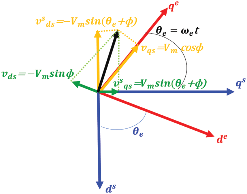
Figure 3: Axes transformation stationary (ds − qs) to synchronously rotating (de − qe) reference frame [17]

Vice versa in Eq. (5):

[vsqsvsds]=[cosθesinθe−sinθecosθe][veqsveds](5)

For dynamic modeling in synchronously rotating reference frame q-axis and d-axis stator flux linkages [18] are shown in Figs. 4 and 5, respectively, which are represented in Eqs. (6)–(8):

λds=Lls.ids+ Lm(1−f(Q))(ids+idr)=(Ls−Lmf(Q)) ids+(Lm(1−f(Q))idr(6)

λqs=Lls.iqs+Lm(iqs+iqr)= Ls iqs+Lm iqr(7)

Total flux linkages of stator side=(λds)2+(λqs)2(8)

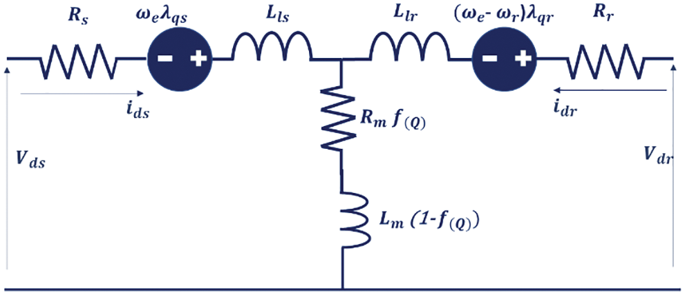
Figure 4: d-axis stator flux linkages [18]

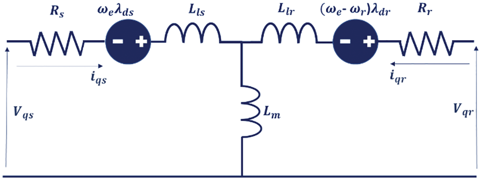
Figure 5: q-axis stator flux linkages [18]

From Figs. 4 and 5 q-and d-axis flux linkages for the rotor are represented mathematically in Eqs. (9)–(11):

λdr=Llr. idr+Lm(1−f(Q))(ids+idr)=(Lr−Lm f(Q)) idr+(Lm(1−f(Q))ids(9)

λqr=Llr iqr+Lm(iqs+iqr)= Lr iqr+Lm iqs(10)

Total flux linkages of rotor side=(λdr)2+(λqr)2(11)

where, Rr and Lr are rotor resistance and inductance, respectively, d represents the primary length in meters and v represents the primary linear speed in m/s. From Figs. 4 and 5, q-and d-axis air gap flux linkages are given in Eqs. (12)–(14):

λqm=Lm(iqs+iqr)(12)

λdm=Lm(ids+idr)(13)

Total flux linkages of air gap=(λdm)2+(λqm)2(14)

With reference to Figs. 4 and 5 the Equation for q-axis and d-axis stator voltages are represented in matrix form as given in Eq. (15):

[vqsvdsvqrvdr]=[(Rs+sLs)ωe(Ls−Lmf(Q))sLm−ωe(Lm−Lmf(Q))−ωeLsRs+sLs+Rrf(Q)−ωeLm sLm+Rrf(Q)−sLmf(Q)sLm(ωe−ωr)(Lm−Lmf(Q))Rr+sLr(ωe−ωr)(Lm−Lmf(Q))−(ωe−ωr)Lm+Rrf(Q)sLm−sLmf(Q) Rrf(Q)(ωe−ωr)LrRrf(Q)(ωe−ωr)][iqsidsiqridr](15)

The matrix equations are transformed for Simulink modeling and are written as Eqs. (16)–(19):

iqs=1Ls∫ vqsdt−RsLs∫ iqsdt−ωeLs(Ls−Lm f(Q))∫ idsdt−LmLsiqr−1Lsωe(Lm−Lm f(Q))∫ idrdt(16)

ids=1Ls∫vdsdt+ωe∫iqsdt−(Rs+Rrf(Q))Ls∫idsdt+ωeLmLs∫iqrdt−LmLsidr−LmLsf(Q))idr+RrLsf(Q)∫idrdt(17)

iqr=1Lr∫vqrdt--LmLriqs--(ωe−ωr)(Lm−Lmf(Q))1Lr∫idsdt−(ωe−ωr)(Lr−Lmf(Q))Lr∫idr.dt−Rr∫iqrdt (18)

idr=1Lm(1−f(Q))∫vdrdt−[--(ωe−ωr)Lm+Rrf(Q)]1Lm(1−f(Q))∫iqsdt+[Lr−Lmf(Q)]1Lm(1−f(Q))ids+Rrf(Q)Lm(1−f(Q))∫idsdt+(ωe−ωr)LrLm(1−f(Q))∫iqrdt−RrLm(1−f(Q)∫idrdt(19)

To develop a complete dynamic model, the mechanical part of the machine is also reflected in modeling. If Fm is mechanical thrust force, J represents rotor inertia, F shows the value of friction constant and vm gives mechanical speed than the following given differential equation represents a mechanical system of induction motor model as given in Eqs. (20)–(21):

ddt vm=12H(Fe−Fvm−Fm)(20)

vm=12H∫(Fe−Fvm−Fm)dt=1J∫(Fe−Fvm−Fm)dt (21)

The expression for thrust force and the motion equation are given as in Eq. (22):

Fe=K(λdriqs−λqrids)= mdvdt+ Dv +FL (22)

In the above Equation, K=3pπ4τp where K represents force constant, p gives no. of pairs, τp indicates pole pitch, D shows viscous friction and iron loss coefficient, and m is the mass of the LIM. By placing values, the thrust force is estimated as follows in Eq. (23):

Fe=32πτpp2(λdriqs−λqrids)(23)

An overall dynamic model of LIM is given in Fig. 6, developed by integrating different Simulink modules.

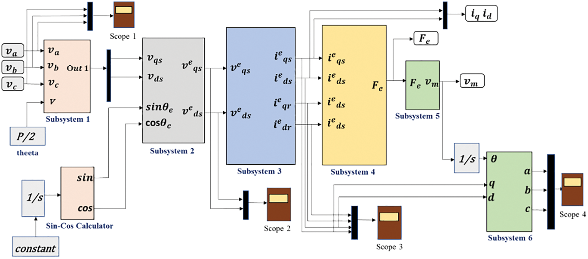
Figure 6: Overall simulink block of dynamic modeling for LIM

3  Space Vector Pulse Width Modulation-Based Inverter for Control of LIM

SVPWM is preferred for PWM implementation over other PWM techniques because of its advantages of improved fundamental output voltage, upgraded harmonic spectrum, and easy implementation in digital signal processors and microcontrollers [19]. SVPWM also provides instantaneous control of switching states and the flexibility for selecting vectors to achieve the balance of the neutral point. It is also possible to yield output voltages nearly for any average value by utilizing the closest three vectors, and this process gives the best spectral performance. SVPWM-based control is provided for LIM, and the main benefit of induction motor control with an SVPWM-based inverter is its improved performance and increased drive lifetime. These advantages motivate the SVPWM-based control scheme for managing electric vehicle-related machines as the proposed control scheme is provided for railway traction systems, and electric vehicles need high starting torque [20,21].

The space vector pulse width modulator is designed based on the SVPWM scheme, and its key parameters are given in Table 2. It comprises seven principle blocks as shown in Fig. 7. The first block is a three-phase generator that provides three sinusoidal waveforms by variable frequency and amplitude, and these three signals are at 120 degrees phase difference. This block has inputs of frequency and voltage required by the inverter. The low-pass bus filter eliminates fast transients from the DC bus voltage calculations. This filtered voltage computes the voltage vectors delivered to the motor [22]. The alpha-beta conversion block transforms variables from the three-phase reference frame to the two-phase reference frame. The plane is allocated into six different sectors separated by 60 degrees. The vector sector finds the sector of the plane having voltage vectors [23]. The switching time calculator gives the timing of the applied voltage vector. The voltage vector lies in the block input sector. The timing sequence from the switching time calculator and ramp signal from the ramp generator is delivered to the gate logic block. This block triggers the inverter switches based on comparing the ramp and the gate timing signals.

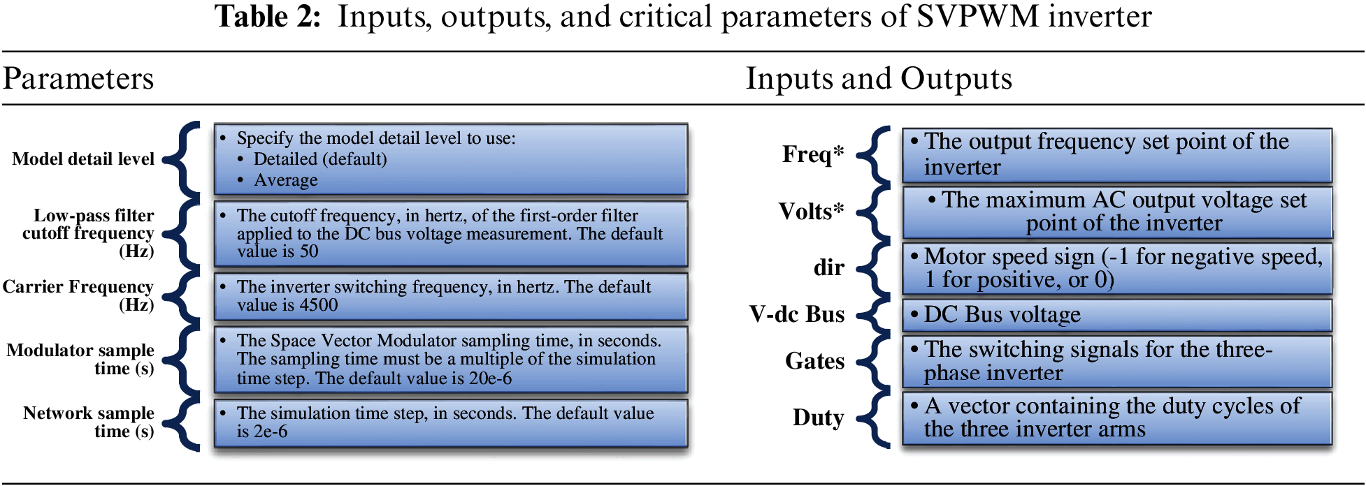
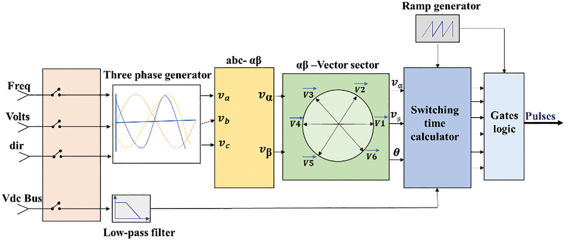
Figure 7: Space vector pulse width modulator structure

When utilizing an average-value inverter, the gates logic block is deactivated, and the inverter leg PWM duty cycles are allotted through the switching time calculator. In this mode, the Space Vector Modulator block outputs the duty cycles of the various pulses but not the pulses themselves. When used in space vector modulation mode, these duty cycle signals are expected by the average-value Three-Phase Inverter block [24]. The complete Simulink block of SVPWM is shown in Fig. 8.

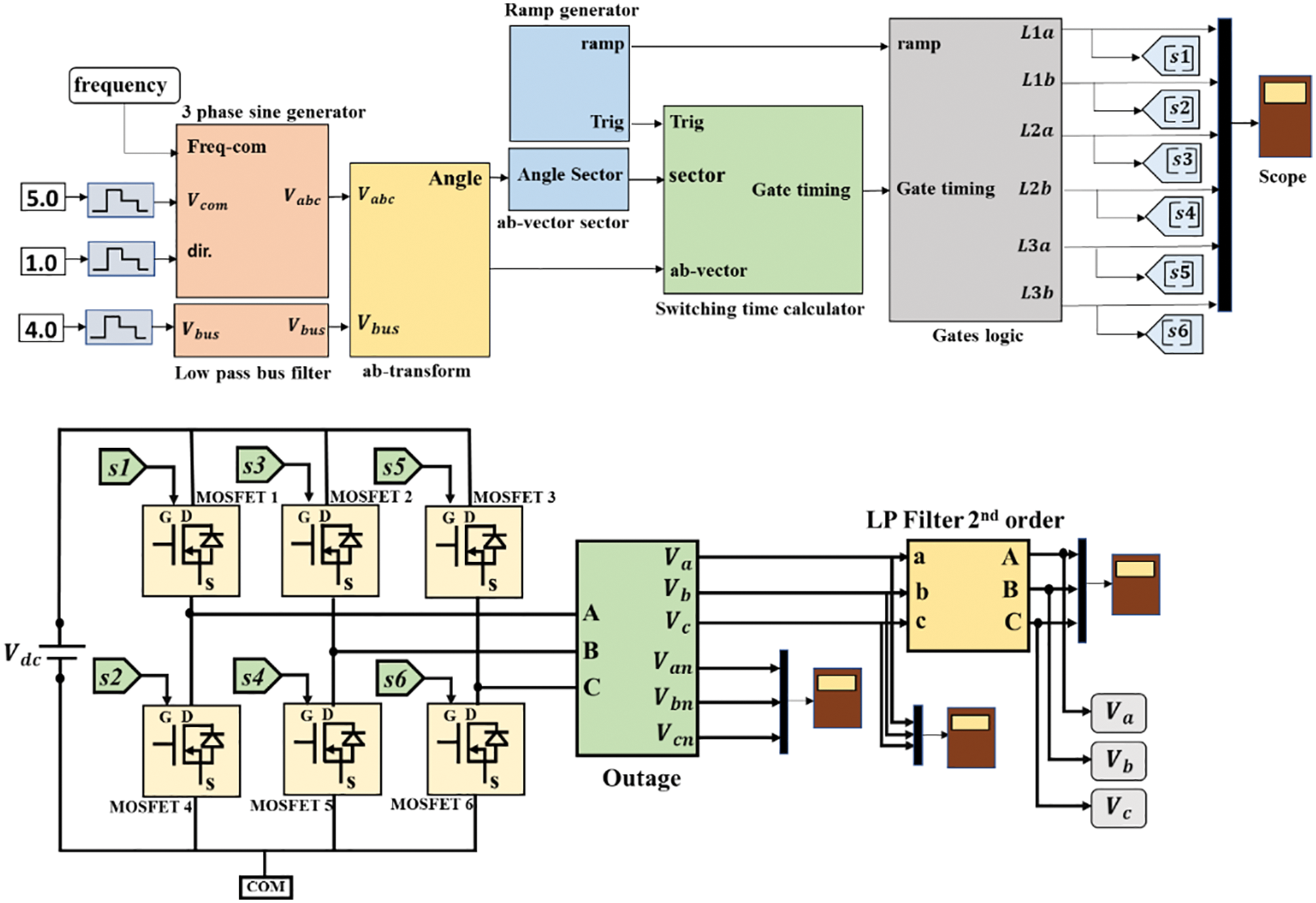
Figure 8: Simulink block of SVPWM

4  PI Controller Design and Tuning for Speed Control

Several approaches are being used to improve controller design and tuning performance [25–27]. An analytical methodology is followed to design a speed controller utilizing the transfer function in which flux linkages are kept fixed and transformed into the separately excited dc motor drive. The speed controller is designed with a systematic optimal approach by using the transfer function as this technique retains the speed-controller design’s consistency for all ac and dc drives [28].

The transfer functions of various subsystems are derived to obtain the block diagram of the indirect vector-controlled induction motor drive. These subsystems mainly include an induction machine, inverter speed controller, and transfer functions for feedback. The final block diagram of the induction motor drive is completed by integrating the subsystems in which the torque-current feedback loop and induced emf feedback loop are overlapped. Block-diagram reduction techniques are used to overcome this overlap in which the inner current loop is made independent of the motor mechanical transfer function, and this method offers a simpler construction of the current controller [29–32].

4.1 Vector-Controlled Induction Motor

For speed controller design of an indirect-controlled induction machine, the key assumption is to maintain constant rotor flux linkages and mathematically can be given as in Eqs. (24)–(25):

r=contant(24)

sr=0(25)

The stator equations of the motor are given as in Eqs. (26)–(27):

veqs=(Rs+sLs)ieqs+ωsLsieds+ sLmieqr+ωsLmiedr(26)

veds=−ωsLsieqs+(Rs+sLs)ieds−ωsLmieqr+sLmiedr(27)

The stator voltage equations can be reformed for the vector control scheme by using the following relationship in Eqs. (28)–(29) of the rotor q and d axis flux linkages.

ieqr=(−LmLr)ieqs(28)

iedr=λrLr−LmLrieds(29)

Modified values of stator voltages after placing values of the rotor currents are given in Eqs. (30)–(31):

veqs=(Rs+sσLs)ieqs+ωsσLsieds+ωsLmLrλr(30)

veds=(Rs+sσLs)ieds−ωsσLsieds+LmLrsλr(31)

where σ is the leakage coefficient. The flux-producing element of the stator current is fixed in steady state condition, which is the d axis stator current in the synchronous frames. Its derivative is also zero, which results as given in Eqs. (32) and (33):

if=ieds(32)

s.ieds=0(33)

The q-axis current in the synchronous frames is the part of the stator current that produces torque, and it is given as in Eq. (34):

iT=ieqs(34)

placing these values into q-axis voltage results via Eq. (35):

veqs=(Rs+ sLa)iT+ωsLaif+ωsLmLrλr(35)

Value of La is given in Eq. (36):

La=σLs=(Ls−Lm2Lr)(36)

The q-axis stator voltage in synchronous frames of reference is found by substituting λr=Lm as in Eq. (37):

veqs=(Rs+ sLa)iT+ωsLaif+ωsLm2Lrif=Rs+ sLaiT+ωsLsif(37)

The Equation of the second stator is not mandatory; the arrangement of both results iT and it is the variable that is controlled in the system. So, the frequency of the stator can be given as in Eq. (38):

ωs=ωr+ωsl=ωr+iTif.RrLr(38)

The electrical equations of the motor are obtained by placing the value of ωe from the above equation results Eq. (39):

veqs=(Rs+sLa)iT+ωrLsif+ωslLsif=(Rs+ sLa)iT+ωrLsif+RrLsLr iT=(Rs+RrLsLr+sLa)iT+ωrLsif(39)

From the above expression, the torque-generating element of the stator current is given as Eq. (40):

iT=veqs−ωrLsifRs+RrLsLr+sLa=Ka1+sTa(veqs−ωrLsif)(40)

where Ra=Rs+RrLsLr, Ka=1Ra and Ta=LaRa. Mathematical expression for electromagnetic force is given from the block that transforms the voltage and speed feedback into the electromagnetic current as Eq. (41):

Fe=KtiT(41)

where electromagnetic constant is given in Eq. (42):

Kt=32P2Lm2Lrif(42)

The load dynamics can be presented given the developed thrust force and a load thrust force that is assumed to be frictional for this specific case as given in Eq. (43):

Jdvmdt+Btvm=Fe−F1= KtiT−Blvm(43)

which is given in Eq. (44) in the form of the electrical rotor speed through multiplication of both sides with the pair of poles.

dvrdt+Bvr=P2KtiT−Blvr(44)

The transfer function between the speed and the thrust force-generating component of current results as Eq. (45):

iT(s)vr(s)=Km1+sTm(45)

where; Km=P2KtBt , Bt=B+Bl and Tm=JBt

4.2 Inverter

The inverter provides stator q-axis voltage as an input signal. The error signal is generated by the reference and thrust force-current feedback, which is the input signal. The generated current error signal is amplified using a current controller. The current controller gain is taken unity, but any other gain value is certainly integrated with the successive progress. Mathematical representation for modeling of the inverter is given as in Eq. (46):

Kin=0.65VdcVcm(46)

where Kin represents the gain of the inverter with a time lag of Tin. Above Equation exhibits that the gain is achieved from the dc-link voltage to the inverter, and the maximum control voltage represented by Vdc and Vcm respectively. The factor of 0.65 gives the maximum peak fundamental voltage available from the inverter through the given dc-link voltage. The torque error signal is limited to the maximum control voltage,Vcm. The time delay in the inverter is equivalent to the average carrier switching-cycle time, i-e, half the period, and is represented using PWM switching frequency as mathematically expressed in Eq. (47):

Tin=12fc(47)

4.3 Speed Controller

The speed error generated by the comparison of the reference and filtered speed feedback command is processed using a proportional-plus-integral (PI) controller, and the transfer function of the speed controller is represented as Eq. (48):

Gs(s)=Ks(1+sTs)sTs(48)

where Ks represents the gain and Ts shows the time constant of the speed controller.

4.4 Feedback Transfer Function

Current and speed are the feedback signals, and these are processed using first-order filters. Usually, minor filtering is provided in the current feedback signal; the gain function of a signal can be given in Eq. (49):

Gc(s)=Hc(49)

Modified speed-feedback signal using a first-order filter can be represented as Eq. (50):

Gω(s)=vrm(s)vr(s)=Hω1+sTω(50)

In above expression Hω represents the gain and Tω gives the time constant for the speed filter.

The speed signals are fed to the speed filter in the form of input, and an improved speed command is developed to compare with the reference signal of speed, ωr∗. It finalizes the progress of all subsystems of the vector-controlled induction machine drives through fixed rotor flux linkages. By combining equations to the mechanical impedance of the load, speed filter, speed controller and iT loop, the block diagram shown in Fig. 9.

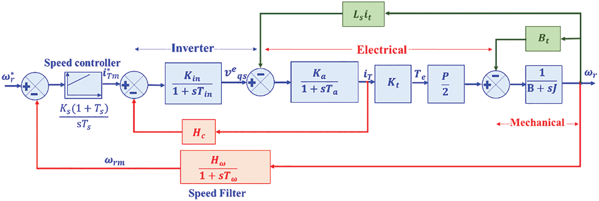
Figure 9: Block diagram of a vector-controlled machine with constant rotor flux linkages

4.5 Block Diagram Reduction

Additionally, the speed-feedback pick-off connection of the electrical system is switched to the iT point providing the diagram given in Fig. 10, which is further reduced and gives the current closed-loop transfer function as presented mathematically in Eq. (51):

Gi(s)=KinKa(1+sTm)(1+sTin)[(1+sTa)(1+sTm)+KaKb]+HcKaKin(1+sTm)(51)

where the electromagnetic force constant is given by Eq. (52):

Kb=KmLsif(52)

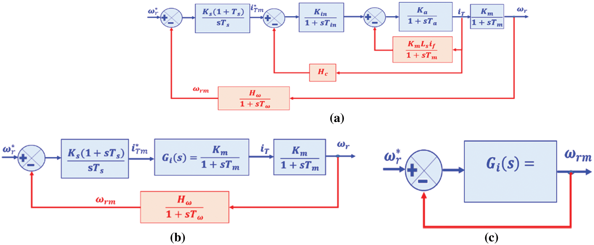
Figure 10: Block diagram reduction of indirect vector-controlled induction motor

4.6 Reduction of Current-Loop Transfer Function

This third-order current transfer function, +iTmHciT∗ , is estimated to first order transfer function as given, Tin is generally neglected in comparison with T1T2 and Tm, and, in the locality of the crossover frequency, the given approximations are effective and presented in Eqs. (53)–(56):

1+ sTin≈1(53)

(1+ sTa)(1+ sTin)≈1+ s(Ta+ Tin)≈1+ sTar(54)

where:

Tar= Ta+ Tin(55)

Placing these results into Gi(s) gives:

Gi(s)=KaKin(1+ sTm)((1+ sTar)(1+ sTm)+ KaKb+HcKaKin(1+ sTm))(56)

which can be written as Eq. (57):

Gi(s)=T1 T2KaKinTar Tm.(1+ sTm(1+ sT1)(1+ sT2))(57)

where Eqs. (58)–(61) are:

−1T1,−1T2=−b±b2−4ac2a(58)

a =TarTm(59)

b= Tar+ Tm+HcKaKinTm(60)

c =1+ KaKb+ HcKaKin(61)

The transfer function Gi(s) is simplified based on the point that T1 < T2 < Tm and close to the locality of the crossover frequency, the effective approximations are given as follows in Eqs. (62)–(63):

1+ sTm≈sTm(62)

1+sT2≈sT2(63)

Placing values into Gi(s) results in Eqs. (64)–(66):

Gi(s)=KaKinT1Tar11+sT1=Ki1+sTi(64)

Ki=KaKinT1Tar(65)

Ti=T1(66)

where KI and TI represent the gain and time constants of the simplified current loop transfer function. The loop transfer function of the speed is set by replacing this simplified transfer function of the current loop and by reducing all the blocks to get the ultimate block diagram as given in Fig. 10.

4.7 Speed Controller Design

The transfer function of the speed loop is mathematically represented by using the following Eq. (67):

GH(s)≈KsTsKg1+sTss2(1+sTωi)(67)

where approximation 1+ sTm≈sTm is considered, and time constants of the current loop and speed filter are integrated into an equivalent time constant as given in Eqs. (68)–(69):

Tωi=Tω+Ti(68)

Kg=KiKmHωTm(69)

The transfer function of the speed to its command can be given as following Eq. (70):

ωr(s)ωr(s)∗=1Hω1+sTs1+sTs+TsKgKss2+TsTωiKgKs.s3(70)

And by relating the coefficients of the denominator polynomial to the coefficient of the symmetric optimum function, Kg and Ts can be assessed as: 1+sTs1+sTs+38Ts2s2+116Ts3s3

From which mathematical expression of speed controller constants are given in Eqs. (71)–(72):

Ts=6Tωi(71)

Ks=491KgTωi(72)

The values of proportional and integral gains for speed controller are derived as Eqs. (73) and (74):

Kp=Ks=491KgTωi(73)

Ki=KsTs=2271KgTωi2(74)

The overshoots can be suppressed by canceling the zero by adding a pole (1 + sTs) in the route of the speed signal.

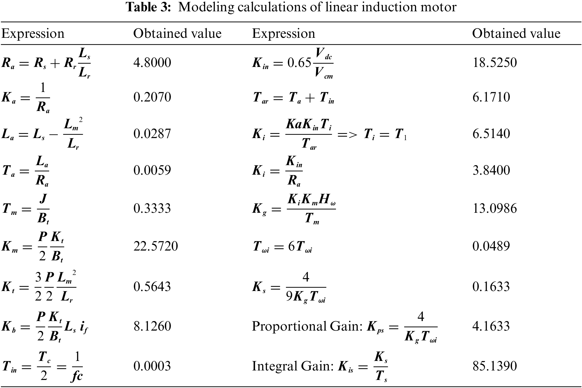
4.8 Optimal Calculations of PI Coefficients for Linear Induction Motor

Considering the parameters of LIM as given in Tables 1 and 2, Optimized values of proportional and integral gain coefficients of the speed controller can be derived as in Table 3.

5  Results and Discussion

The proposed work is completed in three stages. In the first stage, mathematical modeling of a LIM is done in a step-by-step manner. The parameters for the respective machine are given in Table 1, and the presented model was tested in the Simulink environment for the same machine. The simulated LIM exhibited a satisfactory response regarding the torque and speed characteristics. After developing the LIM model, the SVPWM block is developed for the control scheme of LIM, and the output of the respective block is verified. The next step covers the PI controller tuning, using the transfer function of the various subsystems for indirect vector-controlled LIM. The developed dynamic model, SVPWM block, and PI controller with derived parameters are integrated into the Simulink environment as presented in Fig. 11, and Simulation results verify its applicability and robustness. The actual speed of LIM is compared with the step input taken as a reference speed value to get the error signal ultimately transmitted to the PI controller. The controller produces a speed control signal fed to the SVPWM generator as the magnitude of reference vector. The output of SVPWM generator is three modified sinusoidal waveforms of variable frequency and amplitude. These three signals have phase difference of 120°.

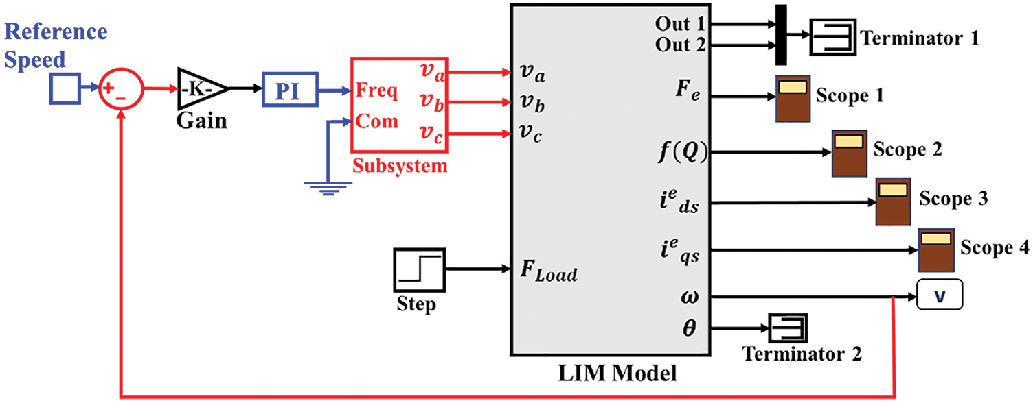
Figure 11: MATLAB/Simulink model of the proposed control scheme

5.1 Outputs of SVPWM Block

Input and output for transformation block of SVPWM inverter as shown in Fig. 8 are presented in Figs. 12–14. Input of the block is a three-phase sinusoidal voltage signal, with a phase difference of 120° among them, and its output is angle selector which is fed to switching time calculator for an accurate decision of gate timings to generate modified line and phase voltage signals.

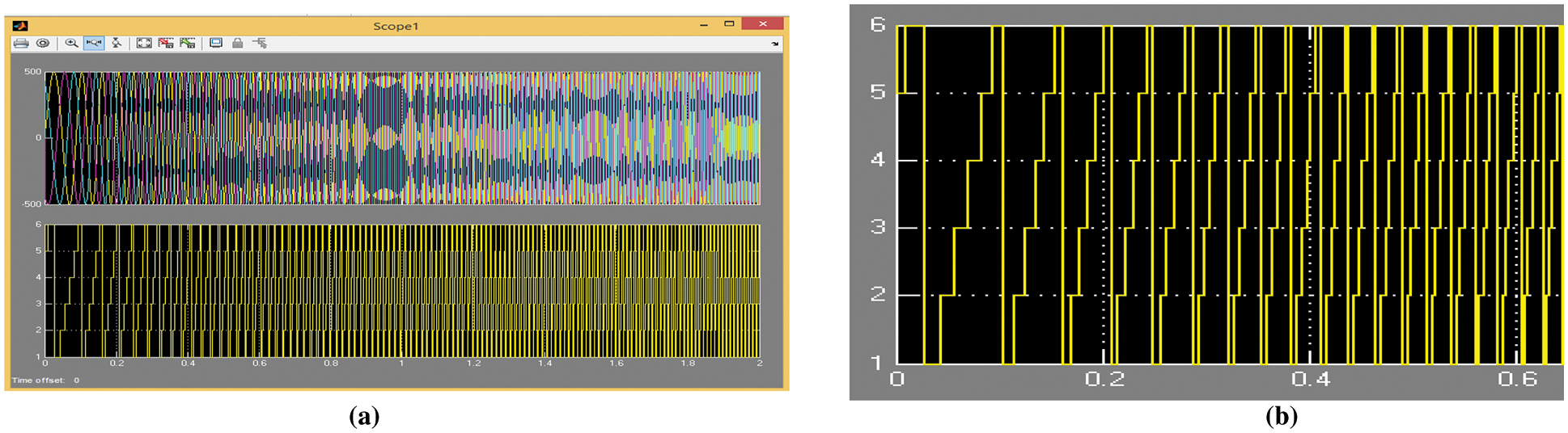
Figure 12: Input (Vabc) and output (angle selector) of transformation block in SVPWM inverter

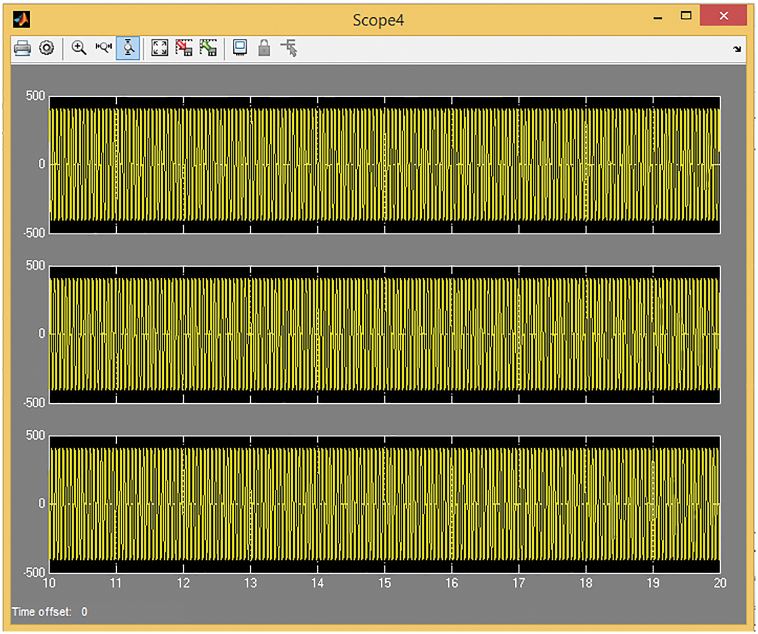
Figure 13: Line voltages output of SVPWM inverter

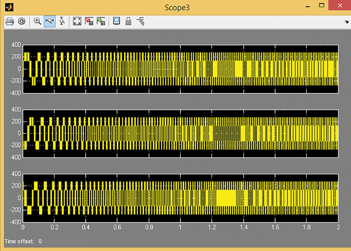
Figure 14: Phase voltages output of SVPWM inverter

5.2 Output at Low Speed

The performance of the proposed system is firstly verified at a low speed of 5 m/s, which is equal to 18 km/h, and the output shown in Fig. 15 exhibits the accurate control of the LIM. Speed output overshoots to the value of 5.8 and is then restored to the reference value in 0.2 s, indicating the prompt response of the proposed control system at the low-speed range. Time response of thrust force at low-speed overshoots to 400 Nm and fluctuates between −10 to 10 Nm once the motor achieves its reference speed.

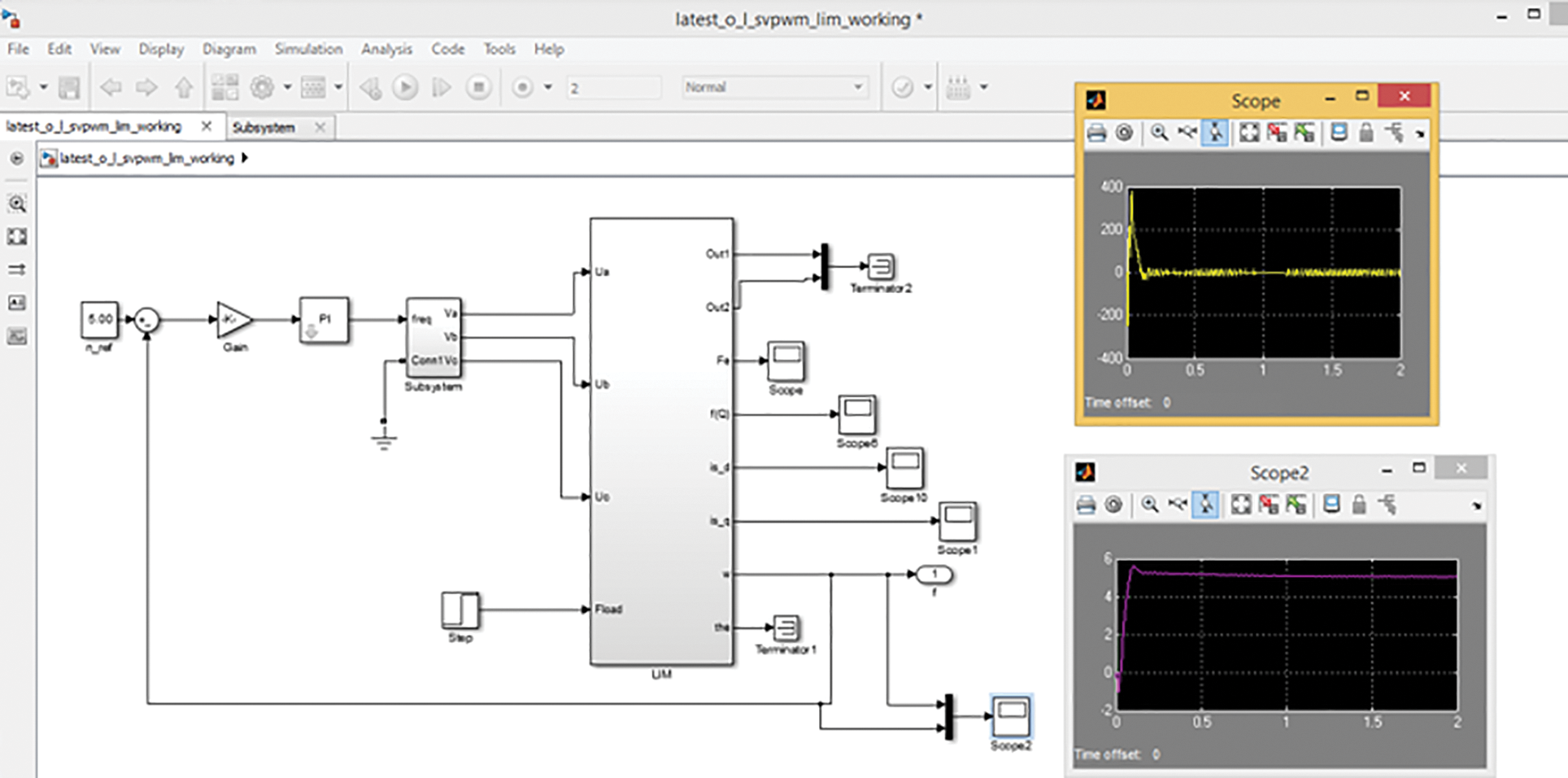
Figure 15: Speed and thrust force output at low-speed range

5.3 Output at High Speed

The dynamic response of the SVPWM-based control scheme is tested considering the end effects of LIM. The simulation results of the motor speed and thrust force at a high-speed range are given in Figs. 16 and 17. To assess the performance of the proposed scheme, Fig. 16 shows that the reference value of LIM speed is selected 100 m/s, equal to 360 km/h, clearly indicates that the selected speed value is higher than conventional range. The green line presents the reference speed, which is followed by the actual speed indicated with the blue line, and it is noted that the motor gained the reference value in 8.5 s.

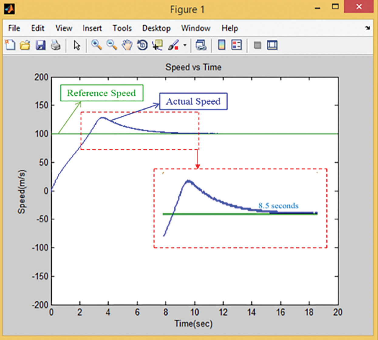
Figure 16: Time response of reference and actual speed

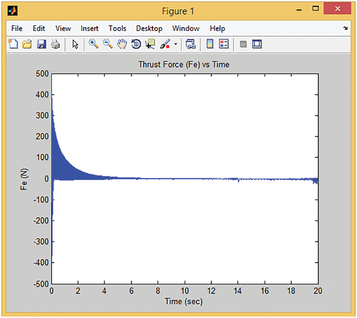
Figure 17: Time response of thrust force at high speed

The thrust force to generate the desired speed is shown in Fig. 17. The maximum amplitude of thrust is less than 400 N, illustrating the controller’s capability to control roughly high-speed LIM with low thrust ripple and oscillation. After achieving the reference value of speed isd and isq have fluctuation range values as shown in Figs. 18 and 19. isd varies in range of −1 to 2 and isq fluctuates in range of −8 to 8 once motor has achieved its reference speed at 8.5 s.

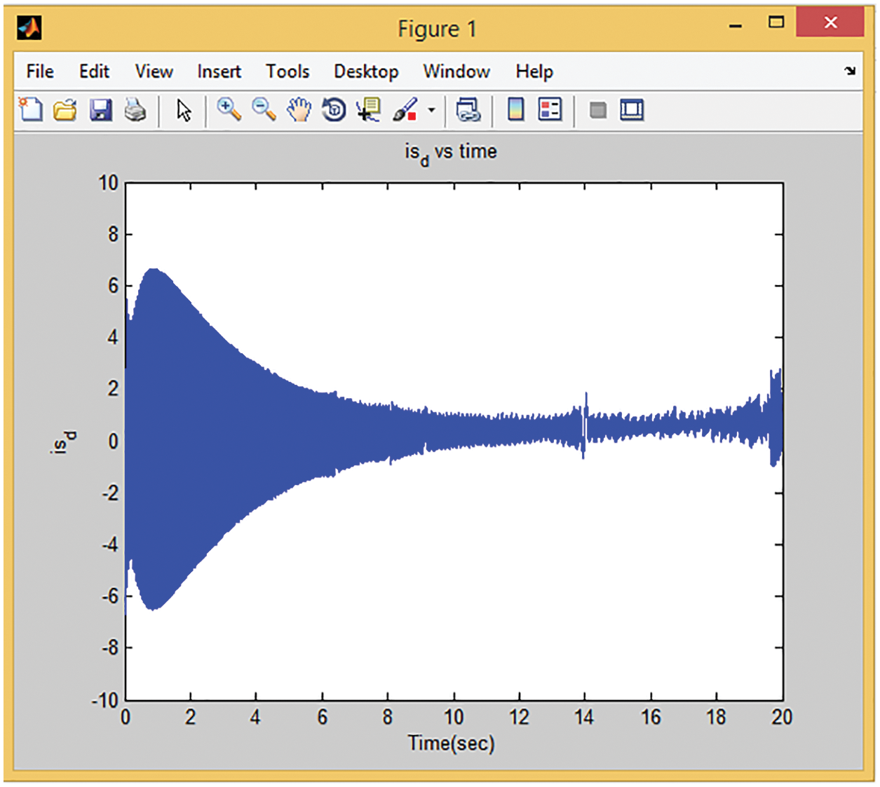
Figure 18: Time response of rotor current

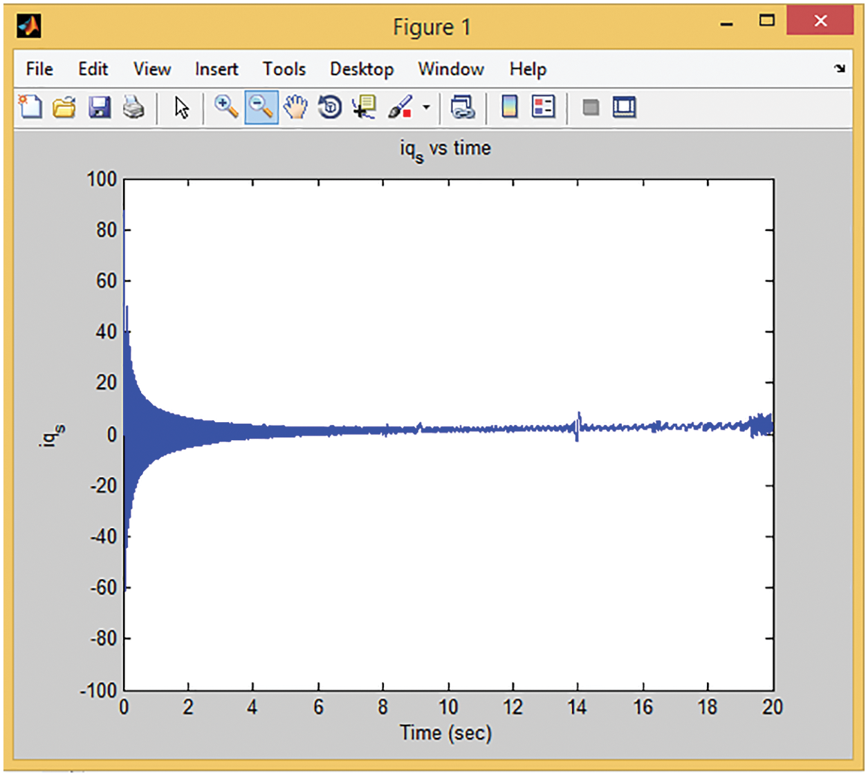
Figure 19: Time response of stator current

In accordance with the study’s objectives, it is determined that the highest thrust amplitude obtained is less than 400 N, indicating the controller’s capacity to regulate a high-speed LIM with minimal thrust ripple. Due to the controlled speed range, the designed system is primarily suggested for low-speed and high-speed, and heavy-duty traction applications.

6  Conclusions

This research develops a novel framework in MATLAB Simulink by integrating three subsystems: an electromechanical model of linear induction motor, an SVPWM-based inverter, and a PI controller. This work aims to achieve precise LIM speed control for low and high-speed applications considering end effects. The developed electromechanical model helps improve the vector control scheme’s transient performance. The model reflects LIM’s final effect, which rises with speed. This effect must be reflected in high-speed control.

The SVPWM generates inverter bridge pulses based on dynamic model command values. SVPWM enables instantaneous switching state control and vector selection flexibility to balance the neutral point. This approach delivers the optimum spectrum performance for generating output voltages for any average value. SVPWM-based inverters are used to manage speed and torque with full dynamic control for high-speed applications.

Integrated controllers have been designed for a six-switch, three-phase inverter loop. The proposed framework is output by altering low and high-speed reference values. The reference value for low-speed performance is 5 m/s, and for high speed, it is 100 m/s. The simulation output motor achieved the reference speed in a few seconds and thrust force less than 500 N, which is acceptable. The proposed framework adjusted the end effects that dominate at high speed. Precise speed control and thrust force prove the framework’s success. Based on its performance, the suggested framework is highly recommended for electric vehicle control; because electric vehicles require high initial torque; thus, this yields the requisite torque at a very high speed, and its control with accommodation of end effects is a significant concern.

Data Availability Statement: No datasets were generated or analyzed during the current study.

Funding Statement: The authors extend their appreciation to the Deanship of Scientific Research at King Khalid University for funding this work through Large Groups Project under grant number (RGP.2/111/43).

Conflicts of Interest: The authors declare that they have no conflicts of interest to report regarding the present study.

References

 1.  Z. Yang, D. Zhang, X. Sun and X. Ye, “Adaptive exponential sliding mode control for a bearingless induction motor based on a disturbance observer,” IEEE Access, vol. 6, pp. 35425–35434, 2018. [Google Scholar]

 2.  H. Hamzehbahmani, “Modeling and simulating of single side short secondary linear induction motor for high speed studies,” European Transactions on Electrical Power, vol. 22, no. 6, pp. 747–757, 2012. [Google Scholar]

 3.  I. Boldea and S. A. Nasar, “Linear electric actuators and generators,” IEEE Transactions on Energy Conversion, vol. 14, no. 3, pp. 712–717, 1999. [Google Scholar]

 4.  H. Gurol, “General atomics linear motor applications: Moving towards deployment,” in Proc. of the IEEE, Torino, Italy, vol. 97, no. 11, pp. 1864–1871, 2009. [Google Scholar]

 5.  M. Anwar, A. H. Abdullah, A. Altameem, K. N. Qureshi, F. Masud et al., “Green communication for wireless body area networks: Energy aware link efficient routing approach,” Sensors, vol. 18, no. 10, pp. 3237, 2018. [Google Scholar]

 6.  M. Anwar, F. Masud, R. A. Butt, S. M. Idrus, M. N. Ahmad et al., “Traffic priority-aware medical data dissemination scheme for IoT based WBASN healthcare applications,” Computers, Materials & Continua, vol. 71, no. 3, pp. 4443–4456, 2022. [Google Scholar]

 7.  K. K. Tan, H. Dou, Y. Chen and T. H. Lee, “High precision linear motor control via relay-tuning and iterative learning based on zero-phase filtering,” IEEE Transactions on Control Systems Technology, vol. 9, no. 2, pp. 244–253, 2001. [Google Scholar]

 8.  R. C. Creppe, J. A. C. Ulson and J. F. Rodrigues, “Influence of design parameters on linear induction motor end effect,” IEEE Transactions on Energy Conversion, vol. 23, no. 2, pp. 358–362, 2008. [Google Scholar]

 9.  M. A. Alqudah, I. Ahmed, F. Ahmad, S. Naseem and K. S. Nisar, “Energy reduction through memory aware real-time scheduling on virtual machine in multi-cores server,” IEEE Access, vol. 9, pp. 55436–55447, 2021. [Google Scholar]

10. M. Faheem, S. B. H. Shah, R. A. Butt, B. Raza, M. Anwar et al., “Smart grid communication and information technologies in the perspective of industry 4.0: Opportunities and challenges,” Computer Science Review, vol. 30, pp. 1–30, 2018. [Google Scholar]

11. M. M. Ud Din, N. Alshammari, S. A. Alanazi, F. Ahmad, S. Naseem et al., “InteliRank: A four-pronged agent for the intelligent ranking of cloud services based on end-users’ feedback,” Sensors, vol. 22, no. 12, pp. 4627, 2022. [Google Scholar]

12. H. Hamzehbahmani, “Modeling and simulating of single side short stator linear induction motor with the end effect,” Journal of Electrical Engineering, vol. 62, no. 5, pp. 302–308, 2011. [Google Scholar]

13. H. Shadabi, A. R. Sadat, A. Pashaei and M. Sharifian, “Speed control of linear induction motor using DTFC method considering end-effect phenomenon,” International Journal on Technical and Physical Problems on Engineering, vol. 7, pp. 75–81, 2014. [Google Scholar]

14. D. Saha, P. Das and S. Chowdhuri, “Design trends of linear induction motor (LIM) and design issues of a single sided LIM,” in Proc. of the 2014 Int. Conf. on Control, Instrumentation, Energy and Communication (CIEC), Calcutta, India, pp. 431–435, 2014. [Google Scholar]

15. X. Wang and F. Blaabjerg, “Harmonic stability in power electronic-based power systems: Concept, modeling, and analysis,” IEEE Transactions on Smart Grid, vol. 10, no. 3, pp. 2858–2870, 2018. [Google Scholar]

16. S. Motlagh and S. S. Fazel, “Indirect vector control of linear induction motor considering end effect,” in 2012 3rd Power Electronics and Drive Systems Technology (PEDSTC), Tehran, Iran, pp. 193–198, 2012. [Google Scholar]

17. H. Shadabi, A. R. Sadat, M. H. Nabavi, M. A. Azari and M. B. Sharifian, “Dynamic performance improvement of linear induction motor using DTFC method and considering end-effect phenomenon,” in 2014 Australasian Universities Power Engineering Conf. (AUPEC), Perth, Australia, pp. 1–6, 2014. [Google Scholar]

18. S. Shah, A. Rashid and M. Bhatti, “Direct quadrate (dq) modeling of 3-phase induction motor using matlab/simulink,” Canadian Journal on Electrical and Electronics Engineering, vol. 3, no. 5, pp. 237–243, 2012. [Google Scholar]

19. K. M. Siddiqui, M. Khursheed, R. Ahmad and F. Rahman, “Performance assessment of variable speed induction motor by advanced modulation techniques,” in Renewable Power for Sustainable Growth, Singapore: Springer, pp. 729–737, 2021. https://doi.org/10.1007/978-981-33-4080-0_70. [Google Scholar]

20. C. Edrington, O. Vodyakho, M. Steurer, S. Azongha, F. Fleming et al., “Power semiconductor loss evaluation in voltage source IGBT converters for three-phase induction motor drives,” in 2009 IEEE Vehicle Power and Propulsion Conf., Dearborn, Michigan, pp. 1434–1439, 2009. [Google Scholar]

21. M. Anwar, A. H. Abdullah, K. N. Qureshi and A. H. Majid, “Wireless body area networks for healthcare applications: An overview,” Telkomnika, vol. 15, no. 3, pp. 1088–1095, 2017. [Google Scholar]

22. S. A. R. Kashif, M. A. Saqib and S. Zia, “Implementing the induction-motor drive with four-switch inverter: An application of neural networks,” Expert Systems with Applications, vol. 38, no. 9, pp. 11137–11148, 2011. [Google Scholar]

23. H. A. Wahab and H. Sanusi, “Simulink model of direct torque control of induction machine,” American Journal of Applied Sciences, vol. 5, no. 8, pp. 1083–1090, 2008. [Google Scholar]

24. M. Anwar, A. H. Abdullah, R. A. Butt, M. W. Ashraf, K. N. Qureshi et al., “Securing data communication in wireless body area networks using digital signatures,” Technical Journal, vol. 23, no. 2, pp. 50–55, 2018. [Google Scholar]

25. G. Liu and S. Daley, “Optimal-tuning PID control for industrial systems,” Control Engineering Practice, vol. 9, no. 11, pp. 1185–1194, 2001. [Google Scholar]

26. M. Tursini, F. Parasiliti and D. Zhang, “Real-time gain tuning of PI controllers for high-performance PMSM drives,” IEEE Transactions on Industry Applications, vol. 38, no. 4, pp. 1018–1026, 2002. [Google Scholar]

27. A. H. Majid, M. Anwar, M. W. Ashraf, “Classified structures and cryptanalysis of Wg-7, Wg-8 and Wg-16 stream ciphers,” Technical Journal, vol. 23, no. 2, pp. 50–55, 2018. [Google Scholar]

28. E. -C. Shin, T. -S. Park, W. -H. Oh and J. -Y. Yoo, “A design method of PI controller for an induction motor with parameter variation,” in IECON’03. 29th Annual Conf. of the IEEE Industrial Electronics Society, Virginia, USA, 2003, vol. 1, pp. 408–413. https://doi.org/10.1109/IECON.2003. [Google Scholar]

29. H. Benbouhenni, Z. Boudjema and A. Belaidi, “A comparative study between four-level NSVM and three-level NSVM technique for a DFIG-based WECSs controlled by indirect vector control,” Carpathian Journal of Electronic and Computer Engineering, vol. 11, no. 2, pp. 13–19, 2018. [Google Scholar]

30. M. Anwar, A. H. Abdullah, R. R. Saedudin, F. Masud and F. Ullah, “CAMP: Congestion avoidance and mitigation protocol for wireless body area networks,” International Journal of Integrated Engineering, vol. 10, no. 6, pp. 59–65, 2018. [Google Scholar]

31. E. Robles, M. Fernandez, J. Andreu, E. Ibarra, J. Zaragoza et al., “Common-mode voltage mitigation in multiphase electric motor drive systems,” Renewable and Sustainable Energy Reviews, vol. 157, pp. 111971, 2022. [Google Scholar]

32. T. Imtiyaz, A. Prakash, F. I. Bakhsh and A. Jain, “Modelling and analysis of indirect field-oriented vector control of induction motor (IM),” in Power Electronics and High Voltage in Smart Grid, Springer: Singapore, pp. 215–228, 2022. [Google Scholar]

Annexure