Efficient Numerical Scheme for Solving Large System of Nonlinear Equations

1  Introduction

Determining the roots of polynomial equations is among the oldest problems in mathematics, whereas polynomial equations have a wide range of applications in science and engineering. For example, aerospace engineers may use polynomials to determine the acceleration of a rocket or jet, and mechanical engineers use polynomials to research and design engines and machines. The search for finding the roots of a system of polynomials and a system of linear or nonlinear equations is one of the primal and difficult problems with wide applications in science, engineering, finance and particular in differential equations. Iterative numerical schemes for solving nonlinear systems of equations associated with initial value problems or boundary value problems are very important because, in general, obtaining a closed form solution using the analytical or exact technique is quite difficult. Generally, nonlinear initial value problems or boundary value problems are solved in two main steps i.e., first to discretize the problem using the difference method, finite difference method, finite element method, Pseudo-Spectral collocation method to the obtained tridiagonal system of linear or nonlinear equations, and in the second step, some numerical iterative numerical schemes are used to solve the tridiagonal system of linear or nonlinear equations.

The first famous, effective and very simple scheme is Newton’s method to solve a nonlinear system of equations is given as:

y(k)=x(k)−F′(x(k))−1F(x(k)),(1)

where F′(x) is the Jacobin matrix approximated at x(k) i.e.,

F′(x)=(∂f1∂x1∂f1∂x2⋯∂f1∂xn∂f2∂x1∂f2∂x2⋯∂f2∂xn⋮⋮⋮⋮∂fn∂x1∂fn∂x2⋯∂fn∂xn)andF(x)=F(x1,…,xn)=(f1(x1,…,xn)f2(x1,…,xn)⋮fn(x1,…,xn))=0.(2)

Method (2), has quadratic convergence locally. A lot of modifications have been made in classical Newton’s Raphson method in order to reduce the number of function and Jacobin evaluations in each iteration step, and so accelerate the convergence order. The extension of the classical Newton method, as described by Weerakoon et al. [1], Özban [2], Gerlach [3] and Young et al. [4], to the function of serval variable has been developed in [5–7] and references therein.

An open closed quadrature-based iterative method was designed by Frontini et al. [8]. This method was improved by Darvishi et al. [9] to obtain a fourth-order scheme. A number of methods, such as the domain decomposition method [10,11], the weight function technique [12], and the replacement of the higher derivative by an approximation [13–15], were used to develop iterative methods to solve a system of nonlinear equation.

The fundamental goal of this study is to construct a higher-order iterative method for solving nonlinear system of equations and highly nonlinear boundary value problems. Basins of attraction are used to demonstrate the efficiency of our method in comparison to the literature’s existing method.

This article is organized as follows: Following the introduction in Section 1, Section 2 provides a brief description of method construction and convergence analysis. The dynamical aspect of the proposed technique’s attraction basins is discussed in Section 3. The numerical outcomes of the proposed method and comparisons to other higher-order existing methods from the literature are shown in Section 4. The paper concludes with Section 5.

2  Construction of Numerical Methods and Convergence Analysis

This section presents some well-known existing iterative schemes of fifth-order convergence.

In 2020, Singh [16] proposed the following fifth-order technique (MSα1):

x(k+1)=w(k)−(F(w(k))F′(x(k))),(3)

where w(k)=z(k)−(F(z(k))F′(x(k))), z(k)=x(k)−(F(x(k))+F(y(k))F′(x(k))) and y(k)=x(k)−(F(x(k))F′(x(k))).

In 2013, Zhang et al. [17] presented the fifth-order iterative technique (MSα2) as below:

x(k+1)=z(k)−(F(z(k))F′(y(k))),(4)

where z(k)=x(k)−12(8F(x(k))F′(x(k))+3(F′(2x(k)+y(k)3)+F′(x(k)+2y(k)3)+F′(y(k)))) and y(k)=x(k)−(F(x(k))F′(x(k))).

Cordero et al. [18] developed the following fifth-order iterative scheme (MSα3) in 2007:

z(k)=x(k)−3(F(x(k))2F′(3x(k)+y(k)4)−F′(x(k)+y(k)2)+2F′(x(k)+3y(k)4)),(5)

where y(k)=x(k)−(F(x(k))F′(x(k))).

Cordero et al. [18] also constructed the following fifth-order iterative scheme (MSα4):

z(k)=x(k)−6(F(x(k))F′(x(k))+4F′(x(k)+y(k)2)+F′(y(k))),(6)

where y(k)=x(k)−(F(x(k))F′(x(k))).

The following scheme (abbreviated as MSα∗) is proposed in the present study:

x(k+1)=y(k)−(8F′(y(k))−6F′(x(k))10F′(y(k))−8F′(x(k))−154(F′(y(k))−F′(x(k))F′(x(k)))2)(F(y(k))F′(x(k))),(7)

where y(k)=x(k)−(F(x(k))F′(x(k))).

Convergence analysis

For the iteration schemes (7), we have the following convergence theorem by using the computer algebra system CAS-Maple 18 and finding the error relation of the iterative schemes defined in (7).

Theorem Let the function F:E⊆Rn→Rn be sufficiently Fréchet differentiable on an open set E containing the root ζ of F(x(k))=0. If the initial estimation x(0) is close to ζ, the method’s MSα∗ convergence order is at least five and satisfies the following:

e⌢(k)=(−186C24−C22C3)(e(k))5+‖O(e(k))6‖,(8)

where Ci=1i!F′(ζ(k))F(i)(ζ(k)),i=2,3,…

Proof: Let e(k)=x(k)−ζ, e∼(k)=y(k)−ζ and e⌢(k)=x(k+1)−ζ be the error in generating Taylor series F(x(k)) in the region of ζ assuming that F′(r)−1 exists, we write:

F(x(k))=Fζ(k)+F′(ζ(k))(x−x(k))+12!F′′(ζ(k))(x−x(k))2+13!F′′′(ζ(k))(x−x(k))3+…(9)

and F(x)=0,

F(x(k))=F′(ζ(k)){e(k)+C2(e(k))2+C3(e(k))3+⋯+C6(e(k))6}+||O(e(k))7||,(10)

Dividing Eq. (9) by [F′(x(k))]−1, we have:

[F′(x(k))]−1F(x(k))=e(k)−C2(e(k))2+(2(C2)2−2C3)(e(k))3+…(11)

e∼(k)=y(k)−ζ=C2+(−2C22+2C3)(e(k))3+…(12)

Expanding F′(y(k)) about ζ and using Eq. (12), we obtain:

F′(y(k))=1+2C22(e∼(k))2+2(−2C22+2C3)(e∼(k))3+…(13)

8(F′(y(k))−6F′(x(k)))]=2−12C2(e∼(k))+(16C22−18C3)(e∼(k))2+(−32C23+32C2C3−24C4)(e∼(k))3+…(14)

10(F′(y(k))−8F′(x(k)))=2−16C2(e∼(k))+(20C22−24C3)(e∼(k))2+(−40C23+40C2C3−32C4)(e∼(k))3+…(15)

15(F′(y(k))−F′(x(k)))]2=60C22(e∼(k))2+(−120C23+180C2C3)(e∼(k))3+(300C24−420C22C3+240C2C4+125C32)(e∼(k))4+||O(e∼(k))5||.(16)

4(F′(x(k)))]2=4+162C(e∼(k))+(16C22+24C3)(e∼(k))2+(48C2C3+32C4)(e∼(k))3+(64C2C4+36C32+40C5)+||O(e∼(k))4||.(17)

Using Eq. (13) and Eq. (15) in the second-step of Eq. (7), we get:

(8F′(y(k))−6F′(x(k))10F′(y(k))−8F′(x(k))−154(F′(y(k))−F′(x(k))F′(x(k)))2)(F(y(k))F′(x(k)))=1+2C(e∼(k))+(−C22+3C3)(e∼(k))2+(186C23−C2C3+4C4)(e∼(k))3+(5C5−285C24+94C32+836C22C3−2C2C4)(e∼(k))4+(5856C25+2267C23C3+1118C22C4+1251C32C2−3C2C5+6C4C3+6C6)(e∼(k))5+…(18)

e⌢(k)=x(k+1)−ζ=(−186C24−C22C3)(e(k))5+||O(e(k))6||.(19)

Hence, it proves the theorem

3  Dynamical Planes

The basins of attraction [19–22] is a graphical representation of how root-finding algorithms respond to different initial estimate points. It is more than a graphical illustration of how a root-finding approach works; it also enables the comparsion of qualitative issues. Visual analysis of dynamical planes, i.e., basins of attraction, is another effective and profitable means of demonstrating the usefulness of iterative methods for solving nonlinear equations with these advantageous properties. A complex square |−3,3×−3,3|2∈C with its centre at the origin and a total of 490000 points is used to generate the dynamical planes. The region on which the first hypotheses are predicted is analyzed in order to locate the root of the nonlinear equation. The stopping criterion |xk+1−xk|<10−3 is utilised to terminate the computer program, and a maximum of 20 iterations are needed root to convergence of the root. Dark black points are assigned, if the orbit of the iterative methods does not converge to root after 20 iterations. Each root is assigned a unique color. In iterative techniques, distinct basins of attraction are illustrated by different colours. Figs. 1–15 illustrate basins of attraction generated by iterative methods for the following non-linear equations:

x5+x3−x−1=0.(20)

Figure 1: The program’s outcome—the basins of attraction for MSα∗ applied to Eq. (20)

Figure 2: The program’s outcome—the basins of attraction for MSα1 applied to Eq. (20)

Figure 3: The program’s outcome—the basins of attraction for MSα2 applied to Eq. (20)

Figure 4: The program’s outcome—the basins of attraction for MSα3 applied to Eq. (20)

Figure 5: The program’s outcome—the basins of attraction for MSα4 applied to Eq. (20)

Figure 6: The program’s outcome—the basins of attraction for MSα∗ applied to Eq. (21)

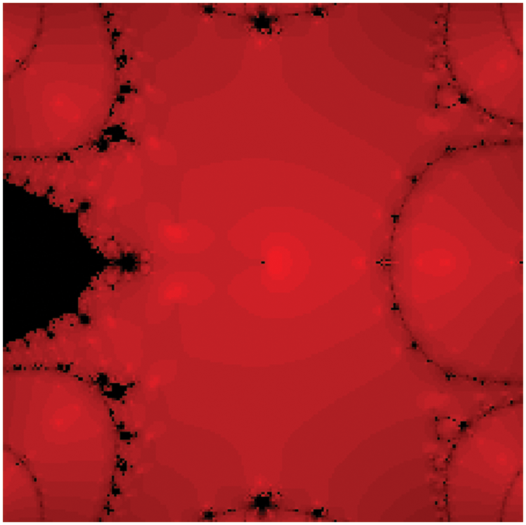
Figure 7: The program’s outcome—the basins of attraction for MSα1 applied to Eq. (21)

Figure 8: The program’s outcome—the basins of attraction for MSα2 applied to Eq. (21)

Figure 9: The program’s outcome—the basins of attraction for MSα3 Eq. (21)

Figure 10: The program’s outcome—the basins of attraction for MSα4 applied Eq. (21)

Figure 11: The program’s outcome—the basins of attraction for MSα∗ applied to Eq. (22)

Figure 12: The program’s outcome—the basins of attraction for MSα1 applied to Eq. (22)

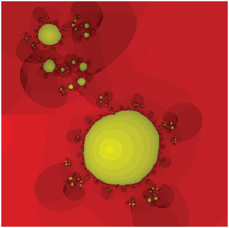
Figure 13: The program’s outcome—the basins of attraction for MSα2 applied to Eq. (22)

Figure 14: The program’s outcome—the basins of attraction for MSα3 applied to Eq. (22)

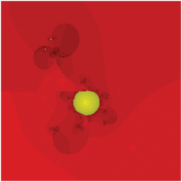
Figure 15: The program’s outcome—the basins of attraction for MSα4 applied to Eq. (22)

Eq. (20) has the following exact roots −0.62174−0.0440597i,−0.621744+0.440597i,0.121744−1.306621i,0.121744+1.30662i,1

cos⁡(x5+x3−x−1)−ex13=0.(21)

Eq. (21) has one real root i.e., 1.135001329.

x35−1x34+2i=0.(22)

Eq. (22) has the following exact roots −2.15564−0.356601i,−0.0918328−0.630339i.

In Tables 1–3, CPU-Time refers to the elapsed time in seconds, Start-Points denote the number of starting points, i.e., 490,000 in a square, Con-Points represent the number of converging points, and Div-Points signify the number of divergent points for the creation of dynamical planes (Attractions’ basins). In terms of CPU-Time, Average-It, Start-Points, Con-Points, and Div-Points, Tables 1–3 clearly show that our newly developed technique MSα∗ outperforms the existing iterative methods MSα1,MSα2,MSα3,MSα4.

4  Numerical Outcomes

The following iterative techniques are used to solve some extremely non-linear boundry value problem BVP and a large system of non-linear equations:

1.    The newly constructed method MSα∗ is of convergence order five

2.    Singh et al.’s method MSα1 is of convergence order five

3.    Zhang et al.’s method MSα2 is of convergence order five

4.    Cordero et al.’s method MSα3 is of convergence order five

5.    Cordero et al.’s method MSα4 is of convergence order five

All numerical computations are done using maple 18.0 with 75-digit floating point arithmetic in a laptop having Processor Intel® Core™ i3-3310 m CPU@2.4 GHz with a 64-bit operating system on Window 8. We terminate the computer program when the following stopping criterion is satisfied:

e=||x(k+1)−x(k)||<∈=10−15,

where e is the absolute error of the consecutive iterations. In Tables 4–8, D represents the dimension of the non-linear system of equations.

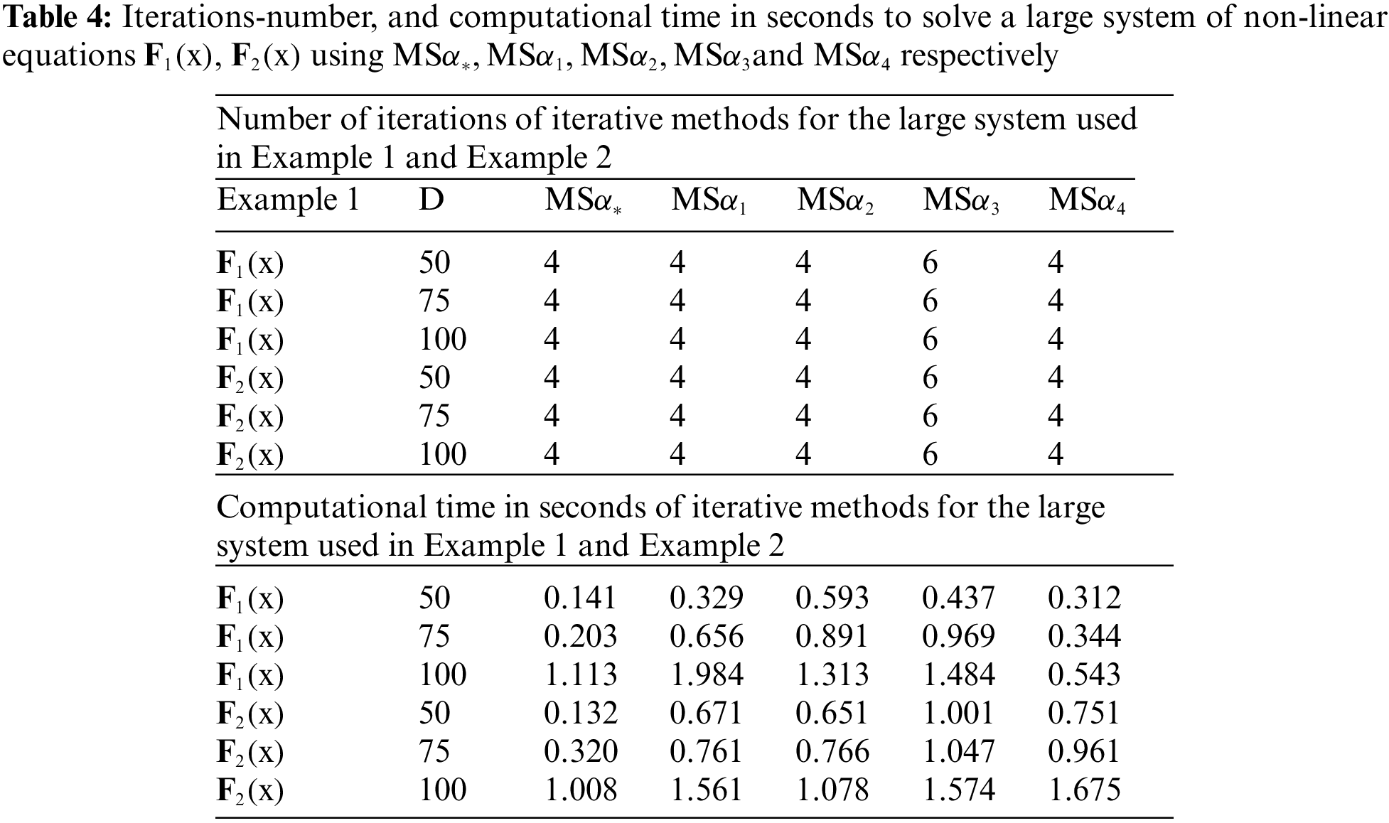
Example 1: N-Demission Problem [23]

Consider

F1:fi(xi)=exi2−1,i=1,2,3,..,m(23)

the exact solution of the system Eq. (23) is X∗=[0,0,0,…,0]T taking X0=[0.5,0.5,0.5,…,0.5] as an initial estimate. Tables 4–5, indicates the numerical results of the system of non-linear equations Eq. (23) used.

Example 2: N-Dimensional Problems [23]

Consider

F2:fi(xi)=xi2−cos⁡(xi−1),i=1,2,3,..,m(24)

the exact solution of the system Eq. (24) is X∗=[1,1,1,…,1]T and taking X0=[2,2,2,…,2]T as an initial estimate. Tables 4–5, indicates the numerical results of the system of non-linear equations Eq. (24) used.

Application in Differential Equation

Here, we solve some highly non-linear BVPs using the newly constructed iterative method and existing methods in literature to show the dominance efficiency of our methods MSα∗ with comparison to MSα1,MSα2,MSα3and MSα4 respectively.

Example 3: [24,25]

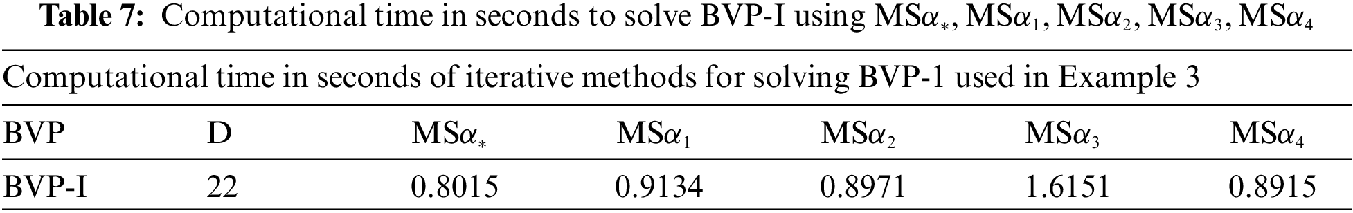
Consider the non-linear boundary value problem (BVP-I):

y′′=−β(ey),0≤x≤1(25)

y(0)=0;y(1)=0. The exact solution to the non-linear boundary value problem does not exist therefore for graphical comparison we take the approximate solutions using the shooting method Fig. 16.

Figure 16: Numerical solution of BVP-1 using shooting methods, MSα∗,MSα1−MSα4.

By dividing the interval [0,1] into n = 22 equal subinterval as:

x0=0<x1<…<xn=1;xi+1=xi+h and h=1n.

Assuming y0=y(x0)=0,y1=y(x1),…,yn=y(xn)=1. Using the procedure of finite-difference central approximations of the derivatives i.e.,

y′′(xi)=1h2(y(xi+1)−2y(xi)+y(xi−1))−h212y(iv)(ξ),for some ξ∈(xi−1,xi+1)(26)

y′(xi)=12h(y(xi+1)−y(xi−1))−h26y(iii)(ξ),for some ξ∈(xi−1,xi+1)(27)

In non-linear boundary value problem Eq. (25), we get the following non-linear system of equations:

484yi+2−968yi+1+848yi+βeyi=0,i=1,2,…,22(28)

We chose the following initial approximation

X0=[0.5,0.5,0.5,0.5,0.5,0.5,0.5,0.5,0.5,0.5,0.5,0.5,0.5,0.5,0.5,0.5,0.5,0.5,0.5,0.5,0.5]T The solution to this non-linear boundary value problem up to 5 decimal places is X∗=[0.00,0.8363576950e−1,0.1650251902,0.2439777869,0.3202933671,0.3937628071,0.4641691297,0.5312888986,0.5948939496,0.6547534661,0.7106363959,0.7623141892,0.8095638206,0.8521710394,0.8899337709,0.9226655761,0.9501990588,0.9723891027,0.9891158112,1.000287032,1.005840356,1.005744498,1.000000000]T

We solve the nonlinear system of equations Eq. (28) by taking β=10.5,10,11. Tables 6–8, indicates the numerical results of the BVP-1 used.

5  Conclusion

A precise approach was developed in this paper for constructing iterative schemes. Using Computer Algebra System CAS-symbolic computation with strong speeding iterative numerical schemes, we developed novel efficient numerical iterative methods for solving nonlinear systems of equations. We were prompted to use symbolic computation via multiple programs written in the computer algebra system CAS-Maple due to the fact that the newly derived technique required lengthy and complicated mathematical statements. Maple was used to perform numerical examples of higher-order nonlinear systems of equations as well as to solve some highly nonlinear BVPs. These examples revealed that the newly developed approaches’ theoretical order of convergence corresponds to the computational outcomes. In addition to providing visual insight into the convergence behavior of iterative methods, the generation of basins of attraction could also generate qualitative concerns for comparison. It is evident from all Figs. 1–16 and Tables 1–8, that the iterative schemes MSα∗ are more effective than MSα1,MSα2,MSα3,MSα4.

Funding Statement: The authors extend their appreciation to the Deanship of Scientific Research at King Khalid University for funding this work through the Large Groups Project under grant number RGP. 2/235/43.

Conflicts of Interest: The authors declare that they have no conflicts of interest to report regarding the present study.

References

1. S. Weerakoon and T. G. I. Fernando, “A variant of newton’s method with accelerated third-order convergence,” Applied Mathematics Letters, vol. 13, no. 8, pp. 87–93, 2000. [Google Scholar]
2. A. Y. Özban, “Some new variants of newton’s method,” Applied Mathematics Letters, vol. 17, no. 6, pp. 677–682, 2004. [Google Scholar]
3. J. Gerlach, “Accelerated convergence in newton’s method,” SIAM Review, vol. 36, no. 2, pp. 272–276, 1994. [Google Scholar]
4. J. Young and M. David, “AM ostrowski, solution of equations and systems of equations,” Bulletin of the American Mathematical Society, vol. 68, no. 4, pp. 306–308, 1962. [Google Scholar]
5. A. Cordero and J. R. Torregrosa, “Variants of newton’s method for functions of several variables,” Applied Mathematics and Computation, vol. 183, no. 1, pp. 199–208, 2006. [Google Scholar]
6. W. Haijun, “New third-order method for solving systems of nonlinear equations,” Numerical Algorithms, vol. 50, no. 3, pp. 271–282, 2009. [Google Scholar]
7. A. Cordero and J. R. Torregrosa, “On interpolation variants of newton’s method for functions of several variables,” Journal of Computational and Applied Mathematics, vol. 234, no. 1, pp. 34–43, 2010. [Google Scholar]
8. M. Frontini and E. Sormani, “Third-order methods from quadrature formulae for solving systems of nonlinear equations,” Applied Mathematics and Computation, vol. 149, no. 3, pp. 771–782, 2004. [Google Scholar]
9. M. T. Darvishi and A. Barati, “A fourth-order method from quadrature formulae to solve systems of nonlinear equations,” Applied Mathematics and Computation, vol. 188, no. 1, pp. 257–261, 2007. [Google Scholar]
10. G. Adomian, “Solution of physical problemes by decomposition,” Computers & Mathematics with Applications, vol. 27, no. 9, pp. 145–154, 1994. [Google Scholar]
11. D. K. R. Babajee, M. Z. Dauhoo, M. T. Darvishi and A. Barati, “A note on the local convergence of iterative methods based on adomian decomposition method and 3-node quadrature rule,” Applied Mathematics and Computation, vol. 200, no. 1, pp. 452–458, 2008. [Google Scholar]
12. A. Cordero, E. Martínez and J. R. Torregrosa, “Iterative methods of order four and five for systems of nonlinear equations,” Journal of Computational and Applied Mathematics, vol. 231, no. 2, pp. 541–551, 2009. [Google Scholar]
13. J. F. Traub, “Computational complexity of iterative processes,” SIAM Journal on Computing, vol. 1, no. 2, pp. 167–179, 1972. [Google Scholar]
14. S. A. Sariman and I. Hashim, “New optimal newton-householder methods for solving nonlinear equations and their dynamics,” Computers, Materials & Continua, vol. 65, no. 1, pp. 69–85, 2020. [Google Scholar]
15. J. R. Sharma, R. K. Guha and R. Sharma, “An efficient fourth order weighted-newton method for systems of nonlinear equations,” Numerical Algorithms, vol. 62, no. 2, pp. 307–323, 2013. [Google Scholar]
16. A. Singh, “An efficient fifth-order iterative scheme for solving a system of nonlinear equations and PDE,” International Journal of Computing Science and Mathematics, vol. 11, no. 4, pp. 316–326, 2020. [Google Scholar]
17. X. Zhang and J. Tan, “The fifth order of three-step iterative methods for solving systems of nonlinear equations,” Mathematica Numerica Sinica, vol. 35, no. 3, pp. 297–304, 2013. [Google Scholar]
18. A. Cordero and J. R. Torregrosa, “Variants of newton’s method using fifth order quadrature formulas,” Applied Mathematics and Computation, vol. 190, no. 1, pp. 686–698, 2007. [Google Scholar]
19. A. Naseem, M. Rehman and T. Abdeljawad, “Computational methods for non-linear equations with some real-world applications and their graphical analysis,” Intelligent Automation & Soft Computing, vol. 30, no. 3, pp. 805–819, 2021. [Google Scholar]
20. Y. M. Chu, N. Rafiq, M. Shams, S. Akram, N. A. Mir et al., “Computer methodologies for the comparison of some efficient derivative free simultaneous iterative methods for finding roots of non-linear equations,” Computers, Materials & Continua, vol. 66, no. 1, pp. 275–290, 2021. [Google Scholar]
21. O. S. Solaiman and I. Hashim, “Optimal eighth-order solver for nonlinear equations with applications in chemical engineering,” Intelligent Automation & Soft Computing, vol. 27, no. 2, pp. 379–390, 2021. [Google Scholar]
22. M. Shams, N. Rafiq, N. A. Mir, B. Ahmad, S. Abbasi et al., “On computer implementation for comparison of inverse numerical schemes for non-linear equations,” CSSE-Computer Systems Science & Engineering, vol. 36, no. 3, pp. 493–507, 2021. [Google Scholar]
23. M. Q. Khirallah and M. A. Hafiz, “Solving system of nonlinear equations using family of jarratt methods,” International Journal of Differential Equations and Applications, vol. 12, no. 2, pp. 69–83, 2013. [Google Scholar]
24. R. L. Burden and J. D. Faires, “Boundary-value problems for ordinary differential equations,” in Numerical Analysis, 9th ed., vol. 1. Boston, MA 02210, USA: Belmount Thomson Brooks/Cole Press, pp. 1–863, 2005. [Google Scholar]
25. Y. Lin, “Enclosing all solutions of two point boundary value problems for ODEs,” Computer and Chemical Engineering, vol. 32, no. 8, pp. 1714–1725, 2008. [Google Scholar]
Cite This Article
Copyright © 2023 The Author(s). Published by Tech Science Press.
This work is licensed under a Creative Commons Attribution 4.0 International License , which permits unrestricted use, distribution, and reproduction in any medium, provided the original work is properly cited.
Downloads
Citation Tools