An Optimization Approach for Convolutional Neural Network Using Non-Dominated Sorted Genetic Algorithm-II

1  Introduction

Numerous scientific domains, including medicine, astronomy, biology, agriculture, and everyday life, have been transformed by digital images. Image classification is a complex process and one of the most frequently performed in applications that use digital images. There has been great progress since the development of convolutional neural networks. The use of CNNs has greatly improved image classification applications. With today’s technology, CNNs are very easy to implement and work with, but for best results you need to choose the optimal architecture and hyperparameters for each individual task. CNN algorithms can be significantly improved if certain hyperparameters (underlying architecture, learning rate, regularization variables, etc.) are well defined. In fact, choosing the right set of hyperparameters can lead to poor or average results, or state-of-the-art performance [1]. In addition to the standard ANN hyperparameters, CNNs include additional hyperparameters such as the number of filters per convolutional layer and filter size. One of the main issues is the time required to evaluate the CNN’s hyperparameter configuration. This is especially true for more complex models that can have many filters per layer. Therefore, CNN inputs are usually simplified or compressed by reducing the image resolution. Recent studies have shown that high-resolution images are beneficial for many classification tasks [2]. This is especially true for images with small regions of interest or where distortion from scaling parameters affects performance. Therefore, practically it is advisable to use high-resolution images, especially when optimizing hyperparameters. In 1989, researchers combined convolutional and backpropagation layers to create the LeNet-5 framework, a neural network applied to MNIST data to improve CNN architecture [3]. CNNs can more easily capture local invariant features, overcome the problems of traditional neural networks, and improve speech and text recognition performance. As the layer depth increases, the gradient vanishes due to the backpropagation process. However, deep learning overcomes the vanishing problem by using ReLU functions as trigger functions and is associated with various applications [4]. However, there is no established method to optimize the hyperparameters, and much research is ongoing. “Manual search” is the traditional optimization strategy.

It is determined by the experimenter’s experience hyperparameters cannot be replicated scientifically, and requires a lot of intuitive observations. Due to the large number of hyperparameters and the lack of deterministic techniques for implementing them, finding the ideal configuration can be difficult. Guess matching techniques are common for tuning CNNs in the early stages of development. Include guesses and estimates. Since this is a difficult problem to optimize, we can use optimization meta-heuristics. Stanley et al. Use reinforcement learning to train recurrent neural networks and identify neural network architectures that are most likely to perform well in professional activities. However, only the hyperparameters of the architecture are optimized, and the learning rate and regularization parameters are finally chosen manually. Moreover, this technique requires a lot of resources. We optimized over 15,000 hyperparameter iterations on hundreds of graphics processing units (GPUs) [5]. Smithson et al. Use neural networks to predict the performance of a set of hyperparameters for a given dataset. Potential hyperparameter samples from the Gaussian containing previously evaluated solutions are sent to the neural network for evaluation. If the neural network uses hyperparameters to predict high performance, the proposed solution is trained, tested, and added to the neural network’s training set. After retraining the neural network predictor on the largest training set, new candidate solutions are selected from the hyperparameter space [6]. Recent studies have shown that obtaining more optimized parameters requires more complex and automated procedures.

Hyperparameters are considered constants that are not updated by training and have a large impact on the accuracy of the algorithm. Various optimization methods are used to optimize hyperparameter tuning for more accurate results. Recent studies have shown that obtaining the optimal hyperparameters requires a more automated and complex procedure rather than manual selection or the guesswork of hyperparameter selection [7]. Most of the basic methods for finding the best hyperparameters are ‘grid search’ and ‘random search’. According to research results, “random search’’ is considered to be more effective than “grid search’’ both experimentally and theoretically [8]. Similarly, “Bayesian optimization” is used for hyperparameter optimization. However, population-based algorithms are better suited for optimizing large numbers of hyperparameters simultaneously, such as CNNs. Recently, reinforcement learning techniques such as Q-learning have been used for hyperparameter optimization [9]. However, while most reinforcement learning techniques excel at optimizing structural parameters, many other parameters such as learning rate and regularization have drawbacks that are user-selectable. “PSO, Simulated Annealing, and Execution Algorithms” are three strategies that have been studied recently. Simple iterative and simple probability-related strategies are suboptimal in hyperparameter optimization In this study, we used the population-based NSGA algorithm to optimize the hyperparameters of the CNN network and classify the MNIST data, cifar-10 and cifar-100 dataset. In addition, we use a computationally accurate CNN network to validate the performance of hyperparameters optimized using the NSGA algorithm.

The contribution of the proposed method can be concluded as follow.

1.    We proposed a hybrid non-dominated sorted genetic algorithm (NSGA) approach to systematically and automatically optimize CNN hyperparameters, improving CNN performance. It makes hyperparameter optimization more feasible for researchers within limited computing resources.

2.    Our approach does not have a constraint on the depth of deep learning models, which means our method can handle problems of different sizes.

3.    An Experimental study is performed to evaluate the performance stability of proposed approach with different schemes on three benchmark datasets. The result shows that the performance of NSGA-CNN is more stable than other traditional CNN architectures on our proposed approach.

2  Background

Hyper parameters are parameters that users must define manually before applying a deep learning model. They are not generated by training. Even if the deep learning model is generated correctly, setting the wrong hyper parameters will prevent training from functioning properly [10]. Training two CNN models with two different sets of hyper parameters results in different accuracy performance. Table 1 shows the results of implementing two CNN models with two different set of hyper parameters. With the same algorithm network structure, you will see slightly different performance. Assuming the rest of the hypermeters are the same, change one of the hyper parameters called learning rate and check the performance of the two CNN networks termed as case 1 and case 2.

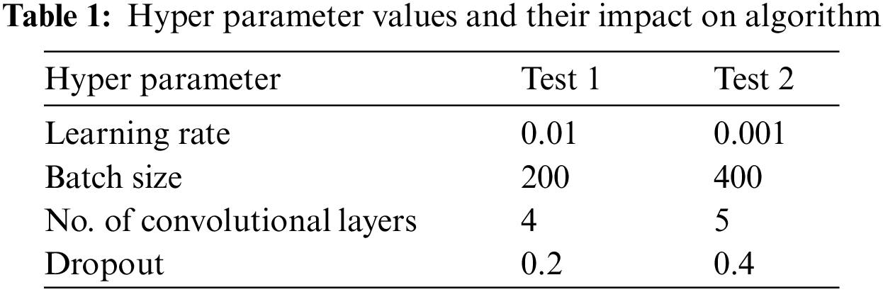
It is clearly indicated from Fig. 1. Due to the numerous ranges and types of hyper parameters, it is very challenging to systematically find the optimal set of values for hyper parameters.

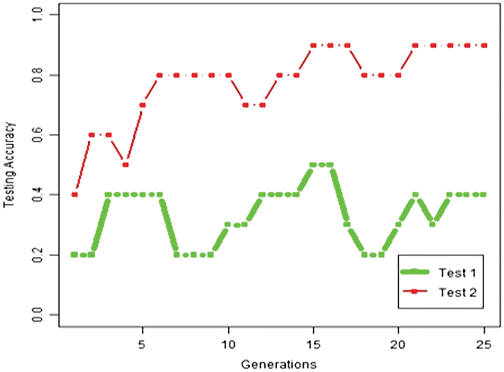
Figure 1: Accuracy changes according to hyperparameter

2.1 Convolutional Neural Network

In recent years, CNN have consistently performed well on a variety of computer vision tasks. CNN’s remarkable performance, especially in automated image processing or video-based recognition and classification systems is not a major factor in CNN’s success. The CNN-based methods require a change in design and engineering focus ahead from hand-crafted features, such as Histogram of Oriented Gradient (HoG) [11,12] for image processing or LaSIFT [13,14] for graphics processing, and toward the heterogeneous network connectivity structures, rigorous training phases with substantial amounts of data, and relevant optimization techniques.

Optimal choice of hyperparameters is one of the main concerns when implementing CNN-based techniques. To our knowledge, there seems to be no reliable way to identify specific network structures that can significantly improve performance. In practice, this means that network architectures are often based more on “educated guesses” than on successful designs. Furthermore, this seems to mean that it is often unclear whether a particular solution yields an ideal or near-optimal configuration, or whether other constructions significantly outperform previous results.

2.2 Non-Dominated Sorted Gentic Algorithm (NSGA-II) Optimization

Over the past decade, many multi-objective evolutionary algorithms (MOEAs) have been introduced. The main motivation for this is to be able to provide many Pareto optimal solutions in one run. The main reason a problem has a multi-objective formulation is that it is impossible to have a single solution that simultaneously optimizes all objectives, so the algorithm provides a large number of alternative solutions that are Pareto-optimal or nearly so is useful for Great practical value. The NSGA algorithm proposed by Srinivas and Deb, was one of the original evolutionary algorithms [15]. The standard NSGA algorithm has faced criticism for its high computational cost in non-dominant sorting, Absence of elitism, and Necessity for Specifying the Sharing Parameter, that explains why we’re adopting NSGA-II to overcome above aforementioned limitations. The most well-known multi-objective optimization algorithm, NSGA-II, is characterised by three key characteristics: a quick non-dominated sorting technique, a quick estimation of the crowded distance parameter, and a quick comparison operator [16]. According to Babajamali et al. [17], the NSGA-II optimization approach performed much better than PAES and SPEA in specifying a larger variety of approaches to several test issues from previous research. It is known as the latest version of Genetic Algorithm because it implements constraints by adjusting the dominant interpretation without requiring a penalty function and has a good mating mechanism that depends on the crowding distance. Compared to evolutionary algorithms, genetic algorithms operate on binary representations of individuals (a string of bits represents each person), which simplifies the combination of mutation and crossover. Such processes generate candidate values outside the permitted search space. In contrast, NSGA algorithms focus on unique data structures that require appropriate mutations and crossovers, which are highly dependent on the situation at hand [18]. The authors of [19] state that the NSGA algorithm can be used when the gradient function is not understood at the point of evaluation. It gives good results because there are many local minima or maxima. In contrast to previous search techniques, features are determined at multiple locations at once instead of one. Since the function computations at each point are generally independent of each other, they can run on multiple processors.

Solution steps for suggested algorithm described in following steps:

Step 1: Initializing the population, Generate the population with the problem’s range and restrictions in consideration.

Step 2: non-dominated sort, sorting approach by using population’s initial non-dominance criteria.

Step 3: Crowd distance, The crowding distance value assigned front-wise whenever the sorting is accomplished. The population is determined according to rank and crowding distance.

Step 4: Selecting A binary tournament selection with crowded-comparison operator is used to choose the individual.

Step 5: Operator Selection, Simulate a binary crossover and integrate a polynomial mutation encoded real GA.

Step 6: Reorganize and Select, Combine the population of the current generation and its descendants to select the individuals that make up the next generation. Each front increases the size of the next generation until the population exceeds the size of the current generation.

Fig. 2 shows the procedure for determining the fitness of the offspring chromosomes. The new parent chromosomes are previous offspring chromosomes and producing a new generation of offspring chromosomes. This is the NSGA method for finding an optimal solution by continuing the phases above.

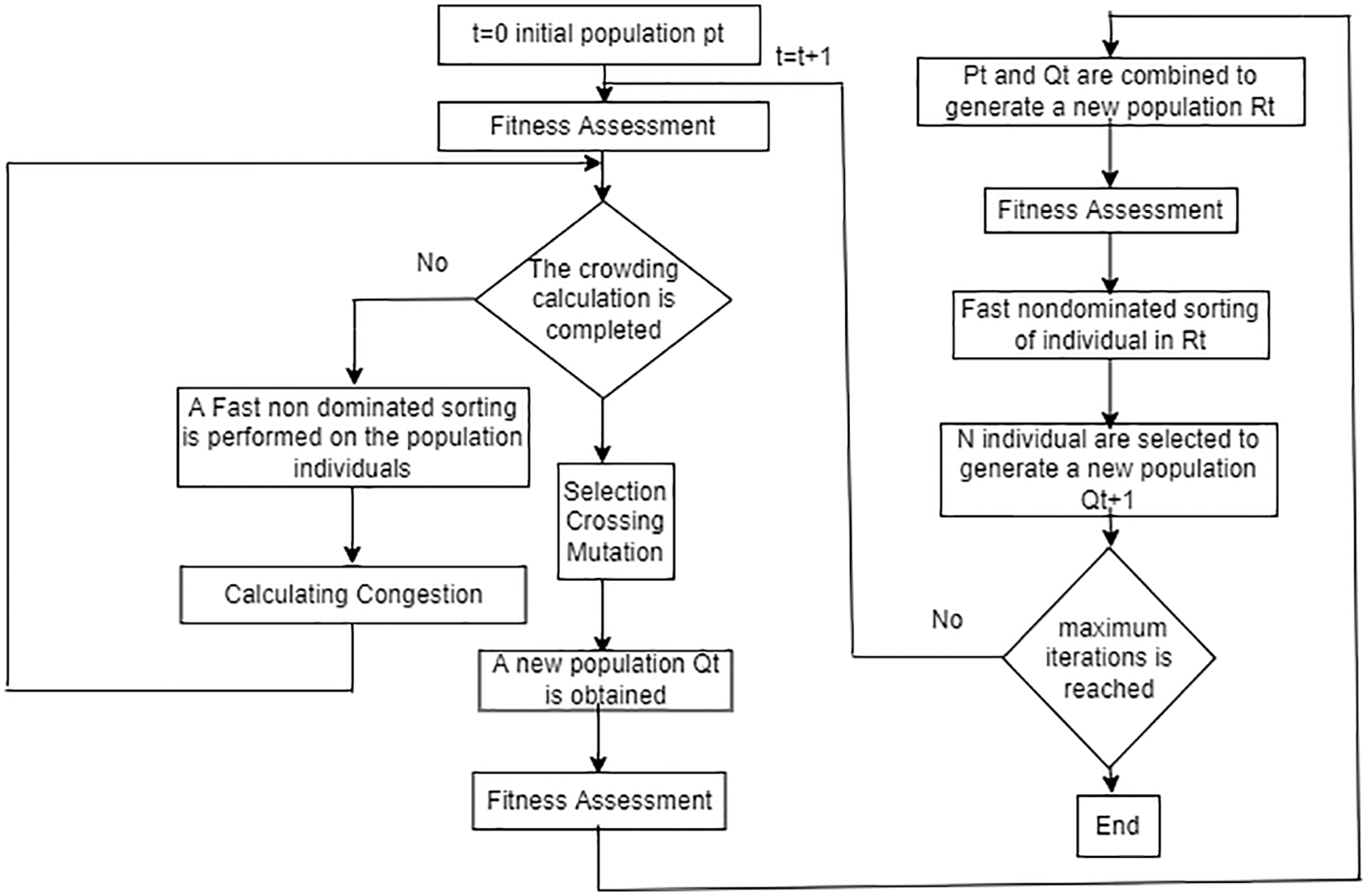
Figure 2: NSGA-II working flowchart

The NSGA-II algorithm is still simple but effective. Route optimization, dynamic channel allocation, training of various neural networks, neuroscience search problems, deep learning hyper parameter optimization, aircraft design by evolving better solutions, neural network weight optimization like great results have been obtained by solving research problems such as optimization. Many challenges have been solved using a NSGA-II algorithm with variable chromosome length.

2.3 Exsisting Hyperparameter Optimization Algorithms

The two most common strategies for hyperparameter optimization are grid search and random search [20]. When using the grid search method, each hyperparameter setting is evaluated over a predefined range of values. Grid search has the advantage of being easy to parallelize. Researchers and experts select edges and transitions between hyperparameter values that form a configuration grid [13]. However, if one job does not go as planned, the others will fail to perform accordingly. Machine learning models typically start with a basic grid and extend it to better lay out the optimal grid while constantly searching for new grids [21]. Because the number of functions to be evaluated increases with each new parameter, we cannot use four hyperparameters due to dimensionality constraints [22].

Random search methods randomly sample the hyperparameter space. According to [23], random search has significant advantages over grid search for applications that can survive the failure of a computer cluster. Solutions can be changed on the fly, new tests can be added to the collection, and failed tests can be ignored. The random search strategy allows concurrent use and flexible termination, making it a whole experiment to be carried out simultaneously. However, if more computers are available, new tests can be added to the experiment without endangering it [24]. Luketina et al. and Fu et al. [25,26] used the gradient descent method to adjust hyperparameters. A framework based on reinforcement learning is used to automatically design the CNN structure. Ma et al. [27] deployed a recurrent neural network to develop a CNN model structure and improved it using reinforcement learning.

Using Bayesian optimization is yet another steady improvement in hyperparameter tuning. It involves use of the Gaussian Process, which is a distribution over functions. Fitting the Gaussian Process to the given data is critical since the resulting function will be very identical to the observed data. The Gaussian process will optimum the predicted improvement and surrogate the model, which is the possibility of a next trial and will optimize the most recent best observation in Bayesian optimization. The next phase will be to use the highest expected improvement, and expected improvement might well be determined anywhere in the search window. Spearmint, which employs the Gaussian process, is a frequent source of Bayesian optimization [28]. The strategy of Bayesian optimization, as according Probost et al. [29] has limitations because it only works with high-dimensional hyperparameters and is extremely computationally expensive. As a consequence, it performs poorly.

Using an evolutionary algorithm to determine the optimal hyperparameters is another approach. Population-based optimization techniques are suitable for optimization problems in high-dimensional variable spaces because they can analyze multiple potential solutions simultaneously. Furthermore, they provide an additional option to combine random searches with previous findings. Chung et al. [30] Kumar et al. [31] and Hinz et al. [32] use genetic algorithms to optimize a subset of hyperparameters in neural networks, showing the general applicability of this approach to problems.

However a small change in hyperparameters can change the efficiency of deep learning algorithms. This means that random searches initially have a large list of instances where hyperparameters determine the correct probability. Therefore, it is difficult to choose random search as the optimal hyperparameter optimization strategy because the first candidate is determined without specific criteria [33]. To solve these problems, hyperparameter optimization studies are conducted based on the algorithm performance of the hyperparameter modification results. In this study, a non-dominated sorted genetic algorithm is used to determine the hyperparameter for CNN which can improve the efficiency and reduce the training time.

3  Optimization Process

Compared to traditional machine learning algorithms, deep machine learning algorithms require more time and space to train the algorithms for multiple important mathematical operations [34]. It is not uncommon for these algorithms and models to take hours or days to solve difficult topics on multiple machines at once. Resolving these issues can be important, but it is time-consuming and memory intensive. Using deep learning algorithms and models, a variety of specialized optimization techniques and approaches have been generated to tackle the problem with less effort and time. These methods and techniques can be successfully used to improve the quality and efficiency of training deep machine learning models. Therefore, Genetic algorithm is used for this research to optimize hyperparameters for CNN. The optimization process for this study consists of data selection, hyperparameter selection and how to create initial population.

3.1 Dataset Selection

This study uses data from the MNIST, Ciphar-10 and Ciphar-100 to train deep CNN networks. The modified National Institute of Standards and Technology (MNIST) benchmark dataset is based on the NIST database. NIST was designed for training and testing (SD-3) using data from Special Database 1 (SD-1) and Special Database 3 (SD-3). SD-3 is less complex than SD-1 because SD-1 is collected from US high school students, while SD-3 is collected from US Census Bureau staff [35]. The conclusions are independent of the proportion of training. The main motivation for combining two NIST datasets and normalizing them to a 28 × 28 pixel image bounding box to generate the MNIST dataset. MNIST data consists of a test set of 60,000 training data and 10,000 black and white handwritten digit data. However, KMNIST contains 70,000 black and white images. Of these, 60,000 will be used for training purposes and the remaining 10,000 will be considered useful for test data.

3.2 Hyperparameter Selection

To perform experiment in this study, the learning rate, dropout rate, batch size, Weight initialization and number of layers are set as hyperparameters.

The learning rate hyperparameters determine the learning speed of the model. Coordinate the generation of allocation errors and update the model weights, for example, at the end of each batch of training samples, each time the parameter is updated. Given a well-designed learning rate, the model is trained to best approximate the functionality of a given available resource for a given number of training periods. If the value is too small, learning will stop before training. Similarly, if the value is too large, the value will diverge and you will not be able to learn effectively.

The concept of “dropout” refers to a neural network unit that is no longer active (both hidden and obvious) [36]. Deleting a unit temporarily removes it from the network, along with all incoming and outgoing connections, as shown in Fig. 3. The units to be dropped are randomly selected. In the most basic example, each unit is held with a fixed probability p. This can be selected using the validation set or set to 0.5. This is true for many networks and the task is almost efficient. On the other hand, the ideal retention probability of an input unit is usually closer to 1 than 0.5. Without dropout, the network overfits with training data and is less efficient with test data. Dropout technique should be used to avoid overfitting and improve accuracy. On the other hand, due to the reduced number of parameters, the impact of dropout on the convolution layer is smaller than the fully connected layer. Therefore, the ratios of dropout rate applied to the layer fully connected to the convolution layer are different.

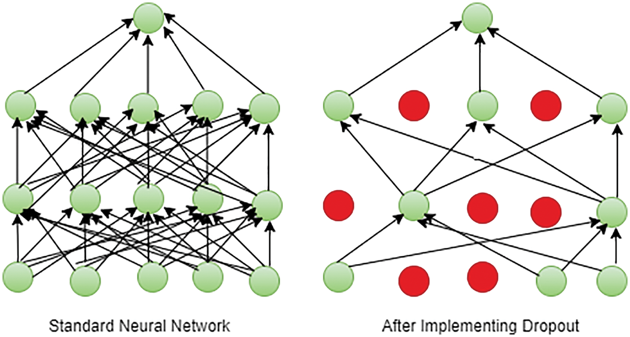
Figure 3: Impact of dropout on standard neural network

The batch size indicates how many samples we can sent to network at once. The model will achieve each epoch faster during training if the batch size is large. This is because, depending on your computing power, the system may be able to process more samples at one time. For training with large amounts of data such as MNIST, researchers prefer to use batch size to avoid computer overload and speed up training [37]. It is chosen for this study to see if the batch size seems to affect your training.

The purpose of weight initialization is to prevent the layer activation output from exploding or vanishing during the training of the deep learning model [38]. If any of these events occur, the loss gradient is too high or too small to move forward and the network will take longer to converge or even show an inability to converge. The process of weight initialization is depicts in Fig. 4.

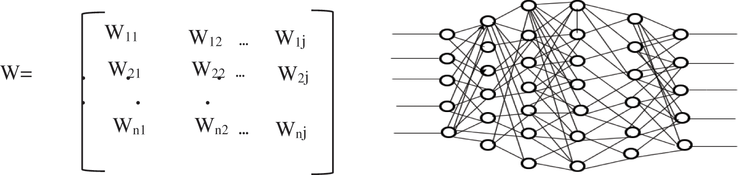
Figure 4: Weight initialization process

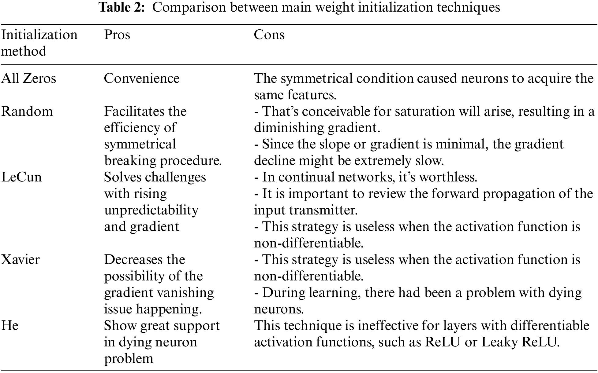
All zeros, random, LeCun, Xavier, and He are perhaps the most often employed weight initialization techniques. The detailed comparison of mentioned techniques are presented in Table 2.

3.3 Create Initial Population

Five genes are to be part of one chromosome. The five genes selected for one chromosomes are learning rate, dropout, batch size, layer and weight initialization. To perform non-dominated sorted genetic algorithm (NSGA) each gene was encoded in a binary format associated with a specific number of bits. The learning rate was observed at 8 bits and ranged from 0.0001 to 0.1. This indicates that there are 28 (= 256) values in the range 0.0001 to 0.1. The drop rate for convolutional levels is drop rate 1 and the drop rate for fully connected levels is drop rate 2. These two values have been classified as 4 bits on a scale of 0 to 0.5. Between 0 and 0.5, there seem to be 24 (= 16) possible values. The batch size is represented by 3 bits and is set to the numbers 50, 100, 200, 250, 400, 500, 1000 and 1250. Similarly, to show this the number of convolution layers has been set to 1, 2, 3 and 4 and represented by 2 bits. A 21-bit chromosome was created by combining these five genes. The chromosomal arrangement is demonstrated in Fig. 5 and Table 3.

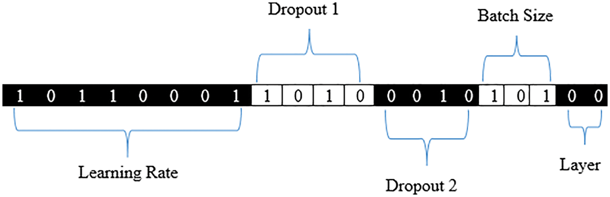
Figure 5: Chromosome arrangement

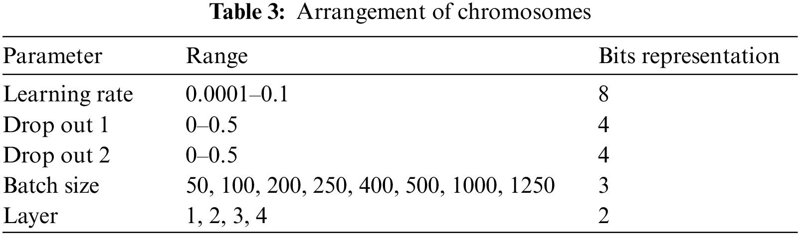
The initial population is made up of 50 chromosomes produced by chosen at random values. Table 3 is depicting arrangement of chromosome for obtaining better results using NSGA algorithm.

3.4 Fitness Evaluation

Fitness should be analysed to assess the generated chromosomes. The accuracy of the test data is used to evaluate fitness in this experiment. The number of valid identified data out of 10,000 testing data is the ratio of accuracy.

Fitness=Number of correctly categorized dataTest data

3.5 Parent Chromosome for Generation

After the successful calculation of fitness value the next generation is generated by selecting the parent chromosomes. Roulette wheel selection method is preferred in this study for selecting parent chromosomes. This became one of the most widely used selection operators, and it is predicated on the proportionality principle. The surface of the roulette wheel proportions corresponds to the fitness value of each individual or potential solution in a population. After the roulette wheel has been spun, the roulette wheel pointer is used to choose a solution. The higher the fitness value and the greater the region, the more probable you are to be chosen. All through the selection phase, the segment size and selection probability remain stationary. This technique’s benefit is that it generates no bias and has an endless spread. This is designed so that if fitness is high, the chances of selection are correspondingly high, and even if fitness is minimal, there is a possibility of still being chosen.

3.6 Offspring Chromosome Generation

By crossing parental chromosome that have been chosen using the roulette wheel selection process, new offspring genes were produced.

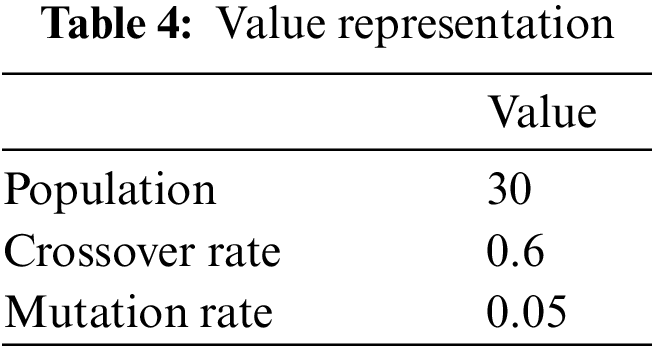
As demonstrated in Fig. 6, the centre of each genome are chosen as crossover regions. The crossovers likelihood was set to 0.6. With a likelihood of 0.05, the mutation procedure is conducted to the newly generated offspring. The contents of the randomly selected bit are reversed during the mutation process.

Figure 6: Chromosome crossover

Mutations affect the fourth element of the learning rate, the first element of dropout 1 and dropout 2, the second element of batch size, and the last element of the layer, as shown in Fig. 7.

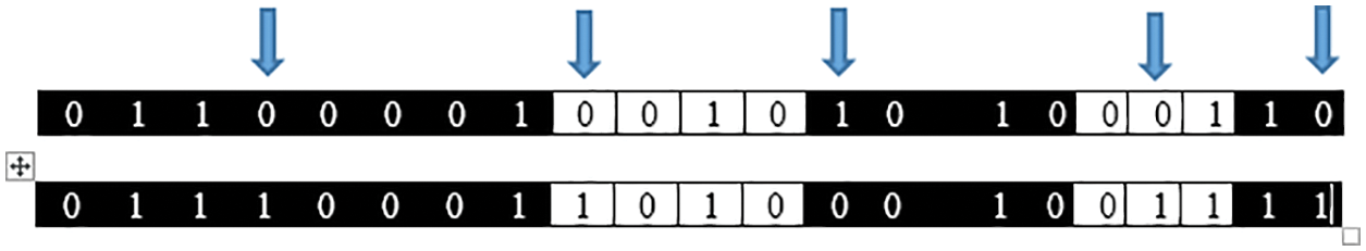
Figure 7: Chromosome mutation

The number of generation is set to 25 to obtain optimal result, as shown in Table 4. The fitness are presented in Table 5.

4  Experimental Result and Analysis

Three experiments were conducted in order to test the effectiveness of this parameter optimization technique. All of the three experiments were tested on 100 generations but we found the desired optimal value at and after 25 generations. We performed a 2-step process to choose the most desired initial value: 1) We sorted the population based on the non-domination, 2) and assign each solution a fitness equal to its non-domination level (minimization of fitness is assumed in this case). The parameters with the highest fitness value were determined for each generation at 25 generations.

Fig. 8, illustrates the variation in fitness of the test data across 25 generations of Genetic Algorithm. It can be observed that the fitness of each generation increases. Three experiments have an accuracy of 0.994 to 0.996.

Figure 8: Fitness by generation (3 Experiments)

Figs. 9–13 presents the values from each hyper-parameter used to determine fitness in Table 6. Each hyper-parameter value changes as the generation grows up, and fitness increases.

Figure 9: Learning rate by generation

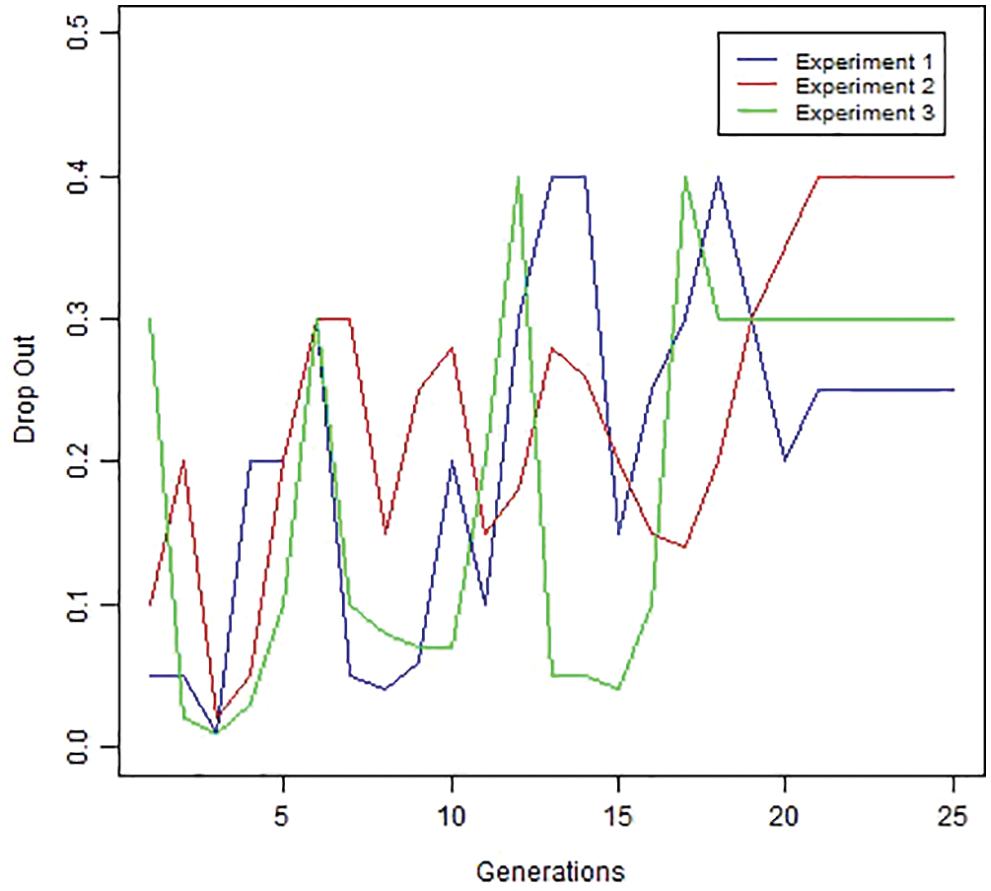
Figure 10: Dropout by generation

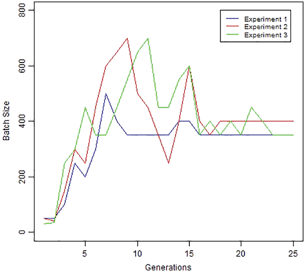
Figure 11: Batch size by generation

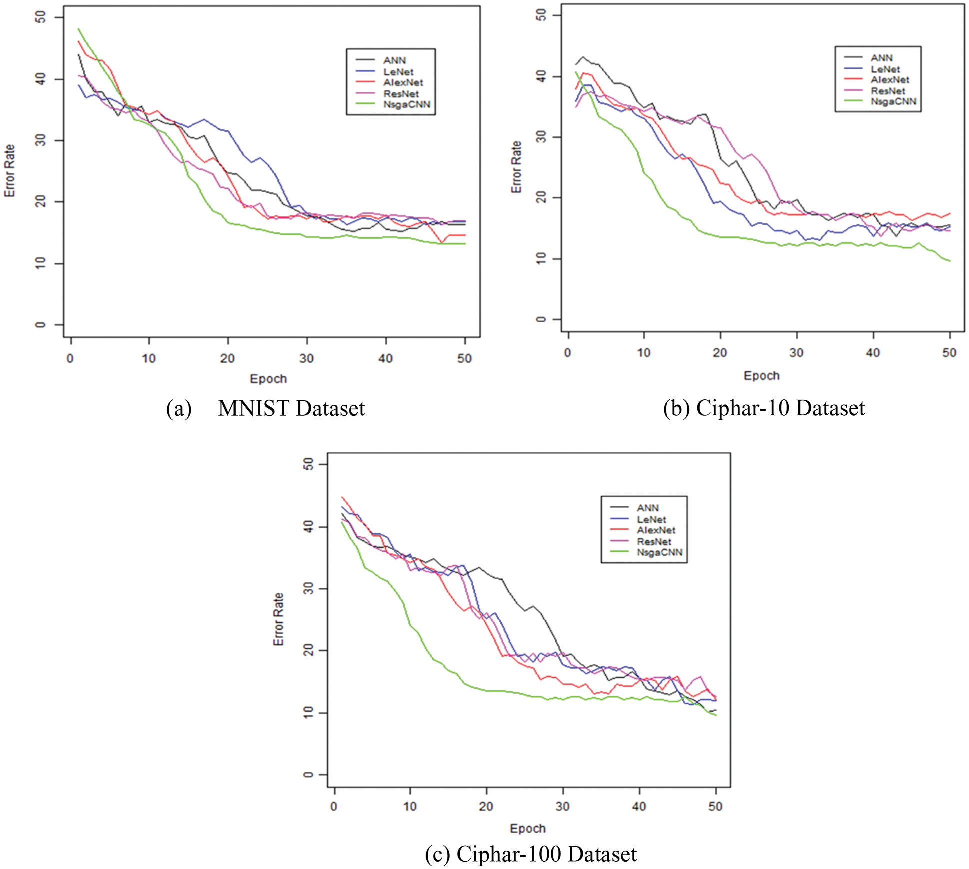
Figure 12: Epoch on MNIST, Ciphar-10 and Ciphar-100 dataset

Figure 13: Accuracy and time complexity on datasets (Ciphar-10, Ciphar-100 and MNIST). Part (a) shows 50% training and testing, Part (b) shows accuracy results on 70% training and 30% testing data, part (c) shows time complexity for standard and proposd approach

The learning rate range was selected between 0.0001 and 0.1, as indicated in Fig. 9, however the optimal learning rate remains relatively low. When the number of generations reaches roughly 18, it is obvious that the learning rate does not fluctuate and remains constant.

The dropout ration to convolutional layer can be seen in Fig. 10. The range difference for each trial is an optimal dropout.

The variation in batch size is seen in Fig. 11. Each experiment has a varied optimal batch size. It has a limited range of possible values. The accuracy of the test data did not enhance by training more data in one go.

5  Comparative Analysis

This section shows the rate of convergence of the competition model established based on the dataset selected from the experiment. The NSGA-II algorithm includes improvements in model accuracy and convergence speed during the training phase for the MNIST, Ciphar-10, and Ciphar-100 datasets, Fig. 12, show the training convergence of all models. All rates of convergence remain the same for each of the 50 iterations. However, after 50 iterations, the error rates for all models remained the same.

With minor changes, the developed model and some competition models work the same for convergence on MNIST datasets. The rates of convergence of all models differed to some extent, and the Ciphar-10 data was much more complex than the MNIST dataset, but proposed NSGA-CNN was able to maintain convergence after 50 iterations. Consistent with the evidence of convergence, the proposed model is superior to other comparable methods in terms of fast convergence speed using NSGA techniques for hyperparameter optimization.

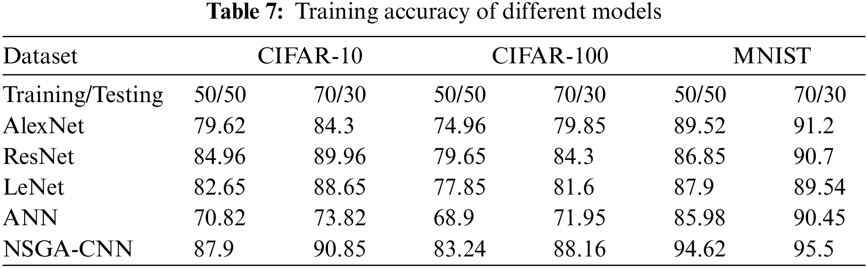
The evaluation of the proposed CNN-NSGA model based on training accuracy. It also shows the definitive finding that the proposed method improves as the complexity and amount of data increases, as shown in Table 7.

The goal of time complexity analysis is to estimate an upper bound on the effort required to evaluate the effectiveness of a proposed algorithm. Comparing various standard algorithms is another target of time complexity analysis for making the most appropriate implementation decisions. The work done provided by the algorithm is used as the basis for time complexity analysis. It will explain the relationship between input size and algorithm execution time to predict constraints.

6  Discussion

The NSGA-II algorithm has been used to approximate solutions to the conventional manual hyperparameter selection problem. This paper studies the multi objective optimization algorithm NSGA-II and optimize the process of hyperparameter selection for standard CNN algorithm. In summary, three experiments were conducted to verify the performance of the hyperparameter optimization method. All of the experiments was tested on 100 generation but the optimal results have been found by after 25 generations. The learning rate was selected between 0.001 and 0.1. Table 6 is representing hyperparameter optimized value. Modelling the CNN by using the achieved mentioned value given in the table has significant accuracy. Three standard datasets were used to evaluate the proposed approach with standard approaches named Cipher 10, Ciphar-100 and MNIST. We can clearly see from Fig. 13 the proposed approach performs better than standard comparative approaches. In order to evaluate our approach we divided data into 50% training and 50% testing (50/50) similarly 70% training and 30% testing (70/30) ratio to see how proposed algorithm effect the accuracy.on both of 50/50 and 70/30 the NSGA-CNN greater accuracy with minmum training time. It depicts that the proposd algorithm will also perform up to the mark on smaller data and optimize hyperparameter efficiently. Time complexity also measured and Table 8 depicts proposed approach reduced training time which would be great advantage for recent advancements.

7  Conclusion

Determining the best architectural design for a machine learning model is difficult as each dataset is different and needs to be tailored to each. Most datasets only need a few hyperparameters. Therefore, different hyperparameters are important for different datasets. There is no mathematical way to determine the appropriate hyperparameters for a given dataset, so trial and error is the only option. Optimization strategies should be adjusted to reduce search space and reduce training time. In this paper, we discover optimal values of CNN hyperparameters for classifying MNIST, Cifar-10 and Cifar-100 data using NSGA algorithm. The learning rate ranges from 0.0004 to 0.0012. You can see that the learning rate of the backpropagation network is decreasing. The loss shows consistent results around 0.2. However, since it uses black and white data, the dropout value is low.

Additionally, training with less than 250 variables at a time guarantees high accuracy. Using a lot of data at once does not lead to high accuracy. With only one or two layers, the structure is too simple to train effectively. The evaluation and selection of the optimal generation in this study took approximately 3990 s. Since the experiment contains a lot of information, estimating the global optimum takes a long time. In the future, we should investigate using NSGA to identify hybrids of global and local optimal search algorithms to find specific optimal values for faster optimization and better results.

Author Contributions: A.Z. Conceptualization; M.A. Implementation; N.M.N. Supervision; A.A. Software, Writing—review & editing; S.R Review & editing; A.R.A Review; A.K.D Editing; B.A review; S.A. Review and funding acquisition.

Acknowledgement: The authors deeply acknowledge the Researchers supporting program (TUMA-Project-2021-27) Almaarefa University, Riyadh, Saudi Arabia for supporting steps of this work.

Funding Statement: This research was supported by the Researchers Supporting Program (TUMA-Project-2021-27) Almaarefa University, Riyadh, Saudi Arabia.

Conflicts of Interest: The authors declare that they have no conflicts of interest to report regarding the present study.

References

 1.  Z. Wang, G. E. Dahl, K. Swersky, C. Lee, Z. Mariet et al., “Automatic prior selection for meta Bayesian optimization with a case study on tuning deep neural network optimizers,” arXiv Preprint arXiv, vol. 11, pp. 2109.08215, September 2021. [Google Scholar]

 2.  H. Talebi and P. Milanfar, “Learning to resize images for computer vision tasks,” in Proc. of the IEEE/CVF Int. Conf. on Computer Vision, Canada, vol. 17, pp. 497–506, May 2021. [Google Scholar]

 3.  Q. Zhang, M. Zhang, T. Chen, Z. Sun, Y. Ma et al., “Recent advances in convolutional neural network acceleration,” Neurocomputing, vol. 323, pp. 37–51, 2019. [Google Scholar]

 4.  L. Alzubaidi, J. Zhang, A. J. Humaidi, AAl-Dujaili, A. Duan et al., “Review of deep learning: Concepts, CNN architectures, challenges, applications, future directions,” Journal of Big Data, vol. 8, pp. 1–74, Springer, March, 2021. [Google Scholar]

 5.  K. O. Stanley, J. Clune, J. Lehman and R. Miikkulainen, “Designing neural networks through neuroevolution,” Nature Machine Intelligence, vol. 1, pp. 24–35, January 2019. [Google Scholar]

 6.  Z. Yin, W. Gross and B. H. Meyer, “Probabilistic sequential multi-objective optimization of convolutional neural networks,” in 2020 Design, Automation & Test in Europe Conf. & Exhibition (DATE), IEEE, vol. 15, Grenoble, France, pp. 1055–1060, 2020. [Google Scholar]

 7.  B. Li, “A more effective random search for machine learning hyperparameters optimization,” Master Thesis, University of Tennessee, Knoxville, vol. 1, December, 2020. [Google Scholar]

 8.  J. Boelrijk, B. Pirok, E. B. Ensing and P. Forre, “Bayesian optimization of comprehensive two-dimensional liquid chromatography separations,” Journal of Chromatography, vol. 1659, pp. 53–72, Elsevier, December, 2021. [Google Scholar]

 9.  A. kumar, A. Zhou, G. Tucker and S. Levine, “Conservative q-learning for offline reinforcement learning,” Advances in Neural Information Processing System, vol. 33, pp. 1179–1191, March, 2020. [Google Scholar]

10. J. Gu, Z. Wang, J. Kuen, A. Shahroudy, B. Shuai et al., “Recent advances in convolutional neural networks,” Pattern Recognition, vol. 77, pp. 354–377, Elsevier, May, 2018. [Google Scholar]

11. T. Zhang, X. Zhang, X. Ke, C. Liu, X. Xu et al., “HOG-ShipCLSNet: A novel deep learning network with hog feature fusion for SAR ship classification,” IEEE Transactions on Geoscience and Remote Sensing, vol. 60, pp. 1–22, IEEE, June 2021. [Google Scholar]

12. J. Sun, Y. Tang, J. Wang, X. Wang, J. Wang et al., “A multi-objective optimisation approach for activity excitation of waste glass mortar,” Journal of Materials Research and Technology, vol. 17, pp. 2280–2304, March 2022. [Google Scholar]

13. A. Axenopoulos, V. Eiselein, A. Penta, E. Koblents, E. Mattina et al., “A framework for large-scale analysis of video\“ in the wild\” to assist digital forensic examination,” IEEE Security & Privacy, vol. 17, no. 1, pp. 23–33, March 2019. [Google Scholar]

14. W. Feng, Y. Wang, J. Sun, Y. Tang, D. Wu et al., “Prediction of thermo-mechanical properties of rubber-modified recycled aggregate concrete,” Construction and Building Materials, vol. 7, no. 318, pp. 125970, February 2022. [Google Scholar]

15. N. Srinivas and K. De, “Muiltiobjective optimization using nondominated sorting in genetic algorithms,” Evolutionary Computation, vol. 2, no. 3, pp. 221–48, September 1994. [Google Scholar]

16. Q. Tashi, E. A. Akhir, S. J. Abdulkadir, S. Mirjalil, T. M. Shami et al., “Classification of reservoir recovery factor for oil and gas reservoirs: A multi-objective feature selection approach,” Journal of Marine Science and Engineering, vol. 18, pp. 888, August 2021. [Google Scholar]

17. Z. Babajamali, F. Aghadavoudi, F. Farhatnia, S. A. Eftekhari and D. Toghraie, “Pareto multi-objective optimization of tandem cold rolling settings for reductions and inter stand tensions using NSGA-II,” ISA Transactions, April 2022. [Google Scholar]

18. A. Dinu, G. M. Danicu and P. L. Ogrutan, “Cost-efficient approaches for fulfillment of functional coverage during verification of digital designs,” Micromachines, vol. 13, pp. 1–32, May 2021. [Google Scholar]

19. J. Islam, P. M. Vasant, B. M. Negash, M. B. Laruccia, M. Myint et al., “A holistic review on artificial intelligence techniques for well placement optimization problem,” Advances in Engineering Software, vol. 41, pp. 102767, March 2020. [Google Scholar]

20. V. Werner, L. Maingault and M. L. Potet, “Fast calibration of fault injection equipment with hyperparameter optimization techniques,” in Int. Conf. on Smart Card Research and Advanced Applications, vol. 12, pp. 121–138, Springer, Lübeck, Germany, November 2021. [Google Scholar]

21. X. Liu, D. Zhang,T. Zhang,Y. Cui, L. Chen et al., “Novel best path selection approach based on hybrid improved A* algorithm and reinforcement learning,” Applied Intelligence, vol. 15, pp. 9015–29, December 2021. [Google Scholar]

22. A. H. Victoria and G. Maragatham, “Automatic tuning of hyperparameters using Bayesian optimization,” Evolving Systems, vol. 12, pp. 217–23, March 2021. [Google Scholar]

23. R. Gerihos, J. H. Jasobsen, C. Michaelis, R. Zemel, W. Brendel et al., “Shortcut learning in deep neural networks,” Nature Machine Intelligence, vol. 11, pp. 665–73, November 2020. [Google Scholar]

24. J. Ratcliffe, F. Soave, N. Brayan, L. Tokachunk and I. Farkhatdinov, “Extended reality (XR) remote research: A survey of drawbacks and opportunities,” in Proc. of the 2021 CHI Conf. on Human Factors in Computing Systems, yokohama, japan, vol. 12, pp. 1–13, May 2021. [Google Scholar]

25. X. Xiao, M. Yan, S. Basodi, C. Ji, Y. Pan et al., “Efficient hyperparameter optimization in deep learning using a variable length genetic algorithm,” Neural and Evaloutionary Computing, vol. 65, pp. 267–284, arxiv, June, 2020. [Google Scholar]

26. C. Zhan, L. Zhang, X. Zao, C. C. Lee, S. Huang et al., “Neural architecture search for inversion,” International Conference on Pattern Recognition, vol. 65, pp. 777–780, ICPR, January, 2022. [Google Scholar]

27. Y. Ma, S. Arshad, S. Muniraju, E. Torkildson, E. Rantala et al., “Location-and person-independent activity recognition with WiFi, deep neural networks, and reinforcement learning,” ACM Transactions on Internet of Things, vol. 2, no. 1, pp. 1–3, ACM, January, 2021. [Google Scholar]

28. A. R. Will, A. G. Kusne, P. Tonner, C. Dong, X. Liang et al., “Application of Bayesian optimization and regression analysis to ferromagnetic materials development,” IEEE Transactions on Magnetics, vol. 13, pp. 1–8, November 2021. [Google Scholar]

29. P. Probost, M. N. Wright and A. L. Boulesteix, “Hyperparameters and tuning strategies for random forest,” in Wiley Interdisciplinary Reviews: Data Mining and Knowledge Discovery, vol. 77, New Jersey, pp. 1–15, Wiley, May, 2019. [Google Scholar]

30. H. Chung and K. S. Shin, “Genetic algorithm-optimized multi-channel convolutional neural network for stock market prediction,” Neural Computing and Applications, vol. 32, no. 12, pp. 7897–914, June 2020. [Google Scholar]

31. P. Kumar, S. Batra and B. Raman, “Deep neural network hyper-parameter tuning through twofold genetic approach,” Soft Computing, vol. 25, no. 13, pp. 8747–71, July 2021. [Google Scholar]

32. T. Hinz, N. Navorro-Guerrero, S. Magg and S. Wermeter, “Speeding up the hyperparameter optimization of deep convolutional neural networks,” International Journal of Computational Intelligence and Applications, vol. 17, pp. 1–15, June 2018. [Google Scholar]

33. S. Sano, T. Kadowaki, K. Tsuda and S. Kimura, “Application of Bayesian optimization for pharmaceutical product development,” Journal of Pharmaceutical Innovation, vol. 15, pp. 333–343, Springer, September, 2020. [Google Scholar]

34. P. Wang, E. Fan and P. Wang, “Comparative analysis of image classification algorithms based on traditional machine learning and deep learning,” Pattern Recognition Letters, vol. 141, pp. 61–67, Elsevier, January 2021. [Google Scholar]

35. E. Hulderson, “Adversarial example resistant hyperparameters and deep learning networks,” (Doctoral Dissertation, University of Washingtonvol. 1, pp. 1–95, ProQuest Dissertations Publishing, 2021. [Google Scholar]

36. R. D. Lange, D. S. Rolnick and K. P. Kording, “Clustering units in neural networks: Upstream vs downstream information,” Neural and Evolutionary Computing, vol. 15, pp. 1–22, Arxiv, March, 2022. [Google Scholar]

37. J. Yu, J. A. Vincent and M. Schwager, “DiNNO: Distributed neural network optimization for multi-robot collaborative learning,” IEEE Robotics and Automation Letters, vol. 7, pp. 896–1903, 2022. [Google Scholar]

38. W. Boulila, M. Driss, E. Alshanqiti, M. Al-Sarem, F. Saeed et al., “Weight initialization techniques for deep learning algorithms in remote sensing: Recent trends and future perspectives,” Advances on Smart and Soft Computing, vol. 1399, pp. 477–484, Springer, 2022. [Google Scholar]