Impact of Artificial Compressibility on the Numerical Solution of Incompressible Nanofluid Flow

Nomenclature

1  Introduction

Heat transfer problems commonly occur in many industries, most notably in the strategic oil and gas and petrochemical industries. In these problems, heat is mainly transferred via convection, conduction, and radiation [1], with convectional heat transfer between fluids and solids being particularly important. Flow inside the cavity has been widely used as a case study to evaluate the performance of new numerical methods [2]. Upwind numerical methods for compressible flows have been widely developed. These methods determine the convective terms at the boundary of the cells by analyzing the propagation of sound waves. For incompressible flows, the speed of sound is infinite, hence these methods cannot be used. On the other hand, in solving the governing equations of incompressible flows, the absence of the pressure term in the continuity equation is problematic. The artificial compressibility method can simultaneously resolve each of these issues. This method changes the type of equations by adding a pressure gradient term to the continuity equation. Adding this term creates a kind of artificial compressibility that allows the definition of virtual sound speed. Therefore, it is possible to apply the various numerical methods used for compressible flows. These benefits motivate the authors to use this scheme. There is no specific restriction for using this method. To determine the pressure at each step of the numerical solution, the Navier-Stokes equations are coupled via an expression connected to the continuity equation, and the governing equations are transformed from elliptical to hyperbolic [3]. The added expression contains a pressure gradient to time and is referred to as the artificial compressibility term. The effect of the artificial compressibility term decreases throughout the numerical solution, and eventually, when the steady-state solution is reached, this term should equal zero, as the gradient of each parameter to time is zero in a steady-state condition. By introducing artificial compressibility, the propagation speed of virtual waves can be determined. In fact, the propagation speed of the waves in an ideal incompressible flow is infinite [4]. The artificial compressibility method, on the other hand, limits the wave propagation speed to a value given by the compressibility coefficient function. The behavior of the boundary layer in viscous fluids is highly sensitive to pressure changes in the flow direction, especially at the separationpoint [5]. If the flow separation occurs, the propagating pressure wave at a finite velocity can change the local pressure gradient and affect the separation point [6]. This phenomenon delays convergence to a steady-state.

Artificial compressibility methods have widely been used by several researchers. Qin et al. [7] compared the SIMPLE and artificial compressibility methods based on their convergence speed and accuracy. Two-dimensional incompressible cavity flow was simulated using these methods in the finite volume framework. The results revealed that the proposed method has a high degree of accuracy and rapid convergence. The optimum value of the artificial compressibility factor was not surveyed by the authors. Ntouras et al. [8] used artificial compressibility to simulate the free surface flow. The simulation was performed to demonstrate the ability of artificial compressibility on unsteady flow with a free surface. The authors showed that the governing equations have hyperbolic nature in a pseudo-time state. When the results of the artificial compressibility approach were compared to experimental and analytical solutions, they showed good accuracy. A constant artificial compressibility factor was used in their study. Some researchers combined artificial compressibility with other methods. For instance, Manzanero et al. [9] combined the artificial compressibility with the discontinuous Galerkin spectral element method to solve incompressible Navier-Stokes equations. A mathematical entropy function was defined to consider the energy terms. The third-order Runge-Kutta method was applied to time marching. The third-order Runge-Kutta method was applied to time marching. As benchmarks, Kovasznay flow, a lid-driven cavity, and the inviscid Taylor–Green vortex were simulated, and good accuracy of the proposed scheme was reported.

Mousa et al. [10] also integrated artificial compressibility with the line approach and utilized the resulting scheme to simulate two-dimensional incompressible flow inside a cavity. The proposed method was used to model magneto-hydrodynamic free convection, and the results were validated against other experimental and numerical results, with good agreement observed. The influence of the artificial compressibility factor was not studied in this work. Jiang et al. [11] combined an artificial compressibility scheme with the Crank-Nicolson Leapfrog method to solve incompressible laminar flows. The results demonstrated that this integrated method is long-term stable and is a second-order scheme. Nagata et al. [12] conducted a theoretical examination of the artificial compressibility system. Following that, a novel explicit artificial compressibility method was proposed, and a two-dimensional flow inside a squared cavity was simulated using the proposed method. Theoretically, they calculated the pseudo speed of sound and used it in their simulations. Reynolds number was considered between 100 and 10,000. The steady and unsteady flows were simulated in this work, and the obtained results demonstrated the accuracy of the proposed method in both cases. Dupuy et al. [13] simulated turbulent flow using an artificial compressibility scheme. To achieve numerical discretization, the finite difference approach in a staggered system was applied. The artificial mach number was defined in this work, and the findings indicated that by extrapolating the artificial mach number, the convergence rate may be accelerated. Additionally, the results demonstrated that the method used to acquire convective fluxes has an effect on the accuracy of the results. Due to the fact that the proposed technique was an explicit mechanism, low memory was required.

Zhang et al. [14] created a new scheme by combining the artificial compressibility method and the spectral collocation approach. They used this scheme to solve three-dimensional incompressible flows numerically. The proposed numerical scheme’s findings were compared to an analytical solution. The combined scheme offered a high degree of accuracy, and the accuracy exponentially increased with time marching. Various computational schemes have been used in the last few decades to discretize virtual governing equations, including averaging methods [15]. According to the history of computing schemes, characteristic methods were initially employed to analyze compressible equations. When the virtual compressibility was added to the incompressible governing equations, the equations were examined using the characteristics approaches as well. Adibi et al. [16,17] studied the Chorin compressibility coupled with a new characteristic base method for two-dimensional flows in order to achieve faster convergence. Their results showed the robustness and high-speed convergence of the proposed scheme. The cavity flow and flow over a cylinder were simulated, and the flow was considered laminar and incompressible. They considered both free and mixed convection in their studies. The artificial compressibility method was considered 5 by the authors.

The literature survey demonstrates the importance of artificial compressibility methods for researchers in different numerical fields. Different researchers also worked on the accuracy of available schemes to improve their accuracy. Marti et al. [18] worked on a finite element-based scheme to improve its accuracy. Three fluid flows with moving boundaries were simulated by the enhanced particle finite element method, and the proposed scheme offered more accuracy. Goona et al. [19] attempted to solve the three-dimensional Poisson equation numerically. By removing error sources, a finite element approach was improved, and a novel scheme was proposed. Numerical simulations of the previous and new proposed schemes were performed, and the results demonstrated that the maximum error can reduce from 8.15% to 0.00091% when the novel scheme is used. Baeza et al. [20] proposed a new scheme for third-order weighted basically nonoscillatory systems. The study revealed that even at a critical time, optimal accuracy occurred for smooth data. As a result, their proposed scheme was based on smoothing the data by adding some nodes with stencil data. Several numerical simulations were conducted using the proposed method, and the results indicated that this scheme is more efficient in error reduction against CPU time. Numerical methods are widely used to investigate flow patterns and heat transfer in a variety of industries due to their advantages, including accessibility to a variety of solutions, low cost, and sensitivity analysis [21–25]. In this context, different numerical methods have been considered to increase the accuracy of the results, reduce the computational costs, and couple the results with analytical methods [26–30]. In these numerical studies, a method has been introduced to solve linear and nonlinear differential equations, which requires a high level of mathematical ability [31–33]. Researchers have combined nanofluids [34–40] and MHD [41–46] with mechanical engineering to improve efficiency in various applications. As a result of these approaches, optimal states for various issues have been found [47–50]. It is even possible for specialists to work and solve common problems in different fields such as medicine [51–53], biotechnology [54,55], and micro-technology [56–58] as a result of advances in numerical calculations and the use of the recent experiences mentioned above. These numerical methods offer acceptable accuracy in solving problems related to thermo-elastic and porous media [59–61]. The accuracy and convergence speed of every numerical scheme is very crucial. Computational fluid dynamics software uses techniques with high convergence speed and good accuracy. In numerical simulations, the artificial compressibility scheme was widely employed. However, the artificial compressibility factor has an impact on its convergence speed and accuracy. Therefore, it is critical to determine the optimal artificial compressible coefficient. Although the artificial compressibility approach is used in various numerical simulations, previous research has not examined the effect of the compressibility factor on the accuracy of results and convergence speed. The effect of the artificial compressibility coefficient on the accuracy of results and the speed of convergence is investigated in the present study. Another novelty of this study is the combination of the artificial compressibility factor with the fifth-order Runge-Kutta method. This novel scheme is formulated in a finite volume framework and convective and viscous fluxes are obtained in cell borders. Numerical simulations are performed for a wide range of Grashof and Reynolds numbers. Consequently, the results of this paper could be used in the numerical solution of natural, mixed, and forced convection in different applications such as heat exchangers. This research allows researchers in the field of numerical methods to ensure the speed of convergence as well as the accuracy of the results by choosing the optimum value for the artificial compressibility factor. It also can be useful for improving the performance of commercial numerical simulation software including ANSYS and COMSOL.

The second section of this work describes the governing equations and the novel numerical technique. In the third section, the problem-solving process and several code components are discussed. In the subsequent stage, the results of numerical simulations are obtained and compared to find suitable answers to the research questions.

2  Problem Formulation

The following equations are applied to two-dimensional and incompressible fluid flow with heat transfer. Density and viscosity are assumed constant for Newtonian fluids with laminar flows. The first equation represents continuity, and the second and third ones signify momentum equations. The fourth equation expresses the energy equation [62].

∂u∂x+∂v∂y=0(1)

∂u∂t+u∂u∂x+v∂v∂y=−1ρ∂p∂x+v(∂2u∂x2+∂2v∂y2)(2)

∂u∂t+u∂u∂x+v∂v∂y=−g−1ρ∂p∂y+v(∂2u∂x2+∂2v∂y2)(3)

∂T∂t+u∂T∂x+v∂T∂y=1ρCp(u∂p∂x+v∂p∂y)+kρCp(∂2T∂x2+∂2T∂y2)+μρCpϕ(4)

where ϕ=[∂u∂x+∂v∂y]2+2[(∂u∂x)2+(∂v∂y)2].

A virtual compressibility sentence (1β∂p∂t) is added to the equation, which tends to zero in the final steady-state solution of this governing equation. In this case, the continuity equation will change as follow:

1β∂p∂t+∂u∂x+∂v∂y=0(5)

For many thermos-flows, a faster convergence can be achieved using the Boussinesq model instead of defining density as a function of temperature.

(ρ−ρo)g≅−ρoβ(T−To)g(6)

where ρo is the (constant) flow density, To is operating temperature, and β is the coefficient of thermal expansion. The above Eq. (4) is obtained using the Boussinesq approximation to remove the buoyancy expression from the momentum equation. This approximation is accurate as long as the change in density is small. To calculate time-dependent thermos flow in confined environments, the Boussinesq approximation is required. As long as the temperature change is small, this model can also be used for steady-state problems. The Boussinesq model cannot be utilized to solve problems involving chemicals or combustion. The governing equation in dimensionless vector form is given by

∂Q∂t+∂F∂x+∂G∂y=∂R∂x+∂S∂y+H(7)

Q¯=[puvT],F=[βup+u2uv(T−EcP)u],G=[βvuyp+u2(T−EcP)v],R=1Re[0∂u∂x∂v∂x1Pr∂T∂x](8)

S=1Re[0∂u∂y∂v∂y1Pr∂T∂y],H=[00GrRe2TEcReϕ],ϕ=[∂u∂x+∂v∂y]2+2[(∂u∂x)2+(∂v∂y)2](9)

In the above relations, Q is the vector of the flow variables, and F, G, R, and S are the convective and viscous flux vectors, respectively; β is the virtual compressibility parameter; Re represents the Reynolds number, and H is the source vector. The set of Eqs. (7)–(9) is obtained using Eq. (10) and the * sign is omitted from all parameters for simplicity. The dimensionless pressure concludes the pressure and the gravitational force of the earth. In other words, the static pressure is obtained first by adding the gravity of the earth to the pressure, and then the dimensionless static pressure is obtained.

u∗=uUref,v∗=vUref,x∗=xUref,y∗=yUref,p∗=p+ρgy−p¥ρrefU2ref,t∗=tUrefLref,T∗=T−Tref1Tref2−Tref1(10)

In Eq. (4), the numbers Gr, Ec, Pr, and Re are dimensionless numbers that are defined by the following relations:

Re=ρrefUrefLrefμ,Pr=Cpμk,Ec=u2refCp(Tref2−Tref1),Gr=βexg(Tref2−Tref1)L3refυ2(11)

where Uref is the upper wall velocity, Lref is the length of the upper wall, and Tref1,Tref2 are the high and low temperatures, respectively. By integrating the governing equations on the cell surfaces, the following equation is obtained:

∂∂t∬QdA+∬(∂(F−R)∂x+∂(G−S)∂y)=∬HdA(12)

The following equation is produced by applying the Green theorem and converting the double integral on the cell surface to the integral on the cell boundaries.

∂∂t∬QdA+∮((F−R)dy−(G−s)dx)=∬HdA(13)

The discretization of the resulting equation in a two-dimensional space with quadrilateral cells leads to the following relation for cells (i, j).

Aij∂Qijk∂t=[∑m=14((Fijk−Rijk)Δy−(Gijk−Sijk)Δx)m−AijHijk],k=1,2,3,4,(14)

The convective terms are obtained by the second-order averaging scheme.

λ∗=(λi,j+λi+1,j)/2→λ=p,u.v−and−T(15)

The fourth-order averaging scheme is used to calculate viscous fluxes on the boundary of secondary cells.

∂η∂x|AB=1S∬s∂η∂xds=1S∮ηdy=1S∑k=14ηΔyk→η=u,v,w(16)

The fifth-order Range-Kutta has been used for time discretization Eq. (12). The main reason behind using this method is that it has a higher convergence rate and larger stability range compared to simple time discretization. Additionally, because the amounts collected in the previous stage and the initial stage are used to determine the quantities in each step, there is no need to store the quantities in the middle stages.

Qijk(p)=Qijk(n)−F(Qijk(p−1)),α=14,16,38,12,1→p=1,2,…,5(17)

In the case of the upper index, P signifies the five steps of the Rang-Kota method, and the index n represents the time step.

A square rectangular cavity with a movable lid is chosen in this study as a benchmark, illustrated in Fig. 1. The fluid contained within the cavity is referred to as an incompressible nanofluid (water-Tio2 nanofluid). Upper and lower walls move at a constant speed of U, while the remaining walls are fixed and insulated. The no-slip law is used to determine the velocity and temperature boundary conditions whereas a second-order extrapolation is used to calculate the pressure.

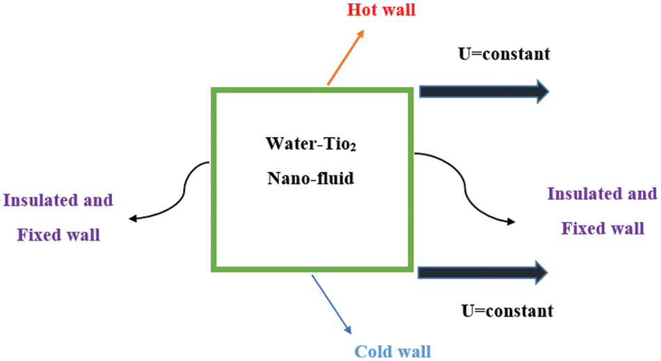
Figure 1: The cavity and its boundary conditions

3  Materials and Methods

The current work is performed in several steps. First, the dimensionless governing equations are discretized in a finite volume framework. Then viscous fluxes and convective fluxes are obtained by a fourth-order and second-order averaging scheme, respectively. Time marching is done by a fifth-order Runge-Kutta method and the velocity, pressure, and temperature fields are obtained. The grid independence and validation of the results are done. In the next step, simulations are repeated for different artificial compressibility factors. Finally, the accuracy and convergence speed are compared for different artificial compressibility factors to find its optimum value. A code has been written in FORTRAN software to perform the above steps. This code contains different subroutines and the main part. The subroutines are then called in the main part. Gird generation is done in the first subroutine. Initial and boundary conditions are given in the second subroutine. Convective fluxes and viscous fluxes are obtained using the third and fourth subroutines. Charts are obtained using these files’ data via TECPLOT software. The flowchart of this work is shown in Fig. 2.

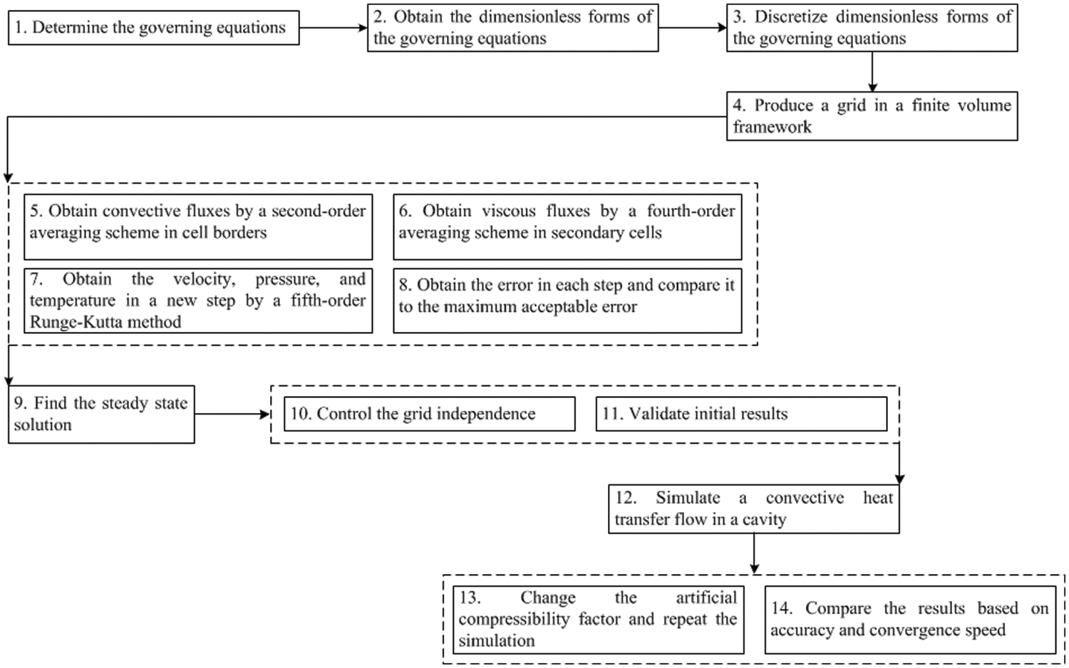
Figure 2: Different steps of current work

4  Results and Discussion

Simulations were run in four distinct grids in order to ensure the accuracy of the numerical solution. The simulations are carried out for β = 5, Gr = 40, Pr = 6.161, Re = 20, and the Nusselt number is calculated, as shown in Fig. 3.

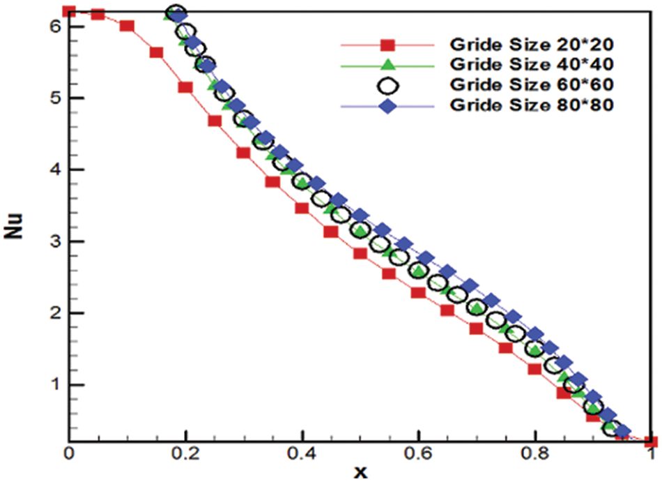
Figure 3: Grid independence (Nusselt number at β=5, Gr = 40, Pr = 6.161, Re = 20)

To find the optimum grid, high accuracy and less computational time are considered. As seen in Fig. 3, the grids 40 × 40, 60 × 60, and 80 × 80 produce approximately similar results. In a 20 × 20 grid, the dimensions of the cells become larger, the error becomes much higher, and thus the grid independence is not obtained. The grid with 40 × 40 (=1600 cells) is chosen for this study because it provides the optimal balance of accuracy and computing time. Finally, validation has been done with the results of Iwatsu et al. [63], as shown in Fig. 4a. The velocity in the vertical centerline of the cavity is calculated and compared to that of Iwatsu et al. [63]. A good agreement is seen between the present and Iwatsu’s results. Different schemes could be used in numerical simulations. Our focus is on the artificial compressibility method in this work. But we compared three different schemes in the first step. The convergence speed of the artificial compressibility method is compared with that of SIMPLE and Lattice Boltzmann schemes in Fig. 4b. This comparison is done in the optimum compressibility factor. Results show better convergence speed for the artificial compressibility method. The error is obtained by

Error=∑i=1Nox∑j=1Noy(ξi,jk+1−ξi,jk)Nox.Noy(18)

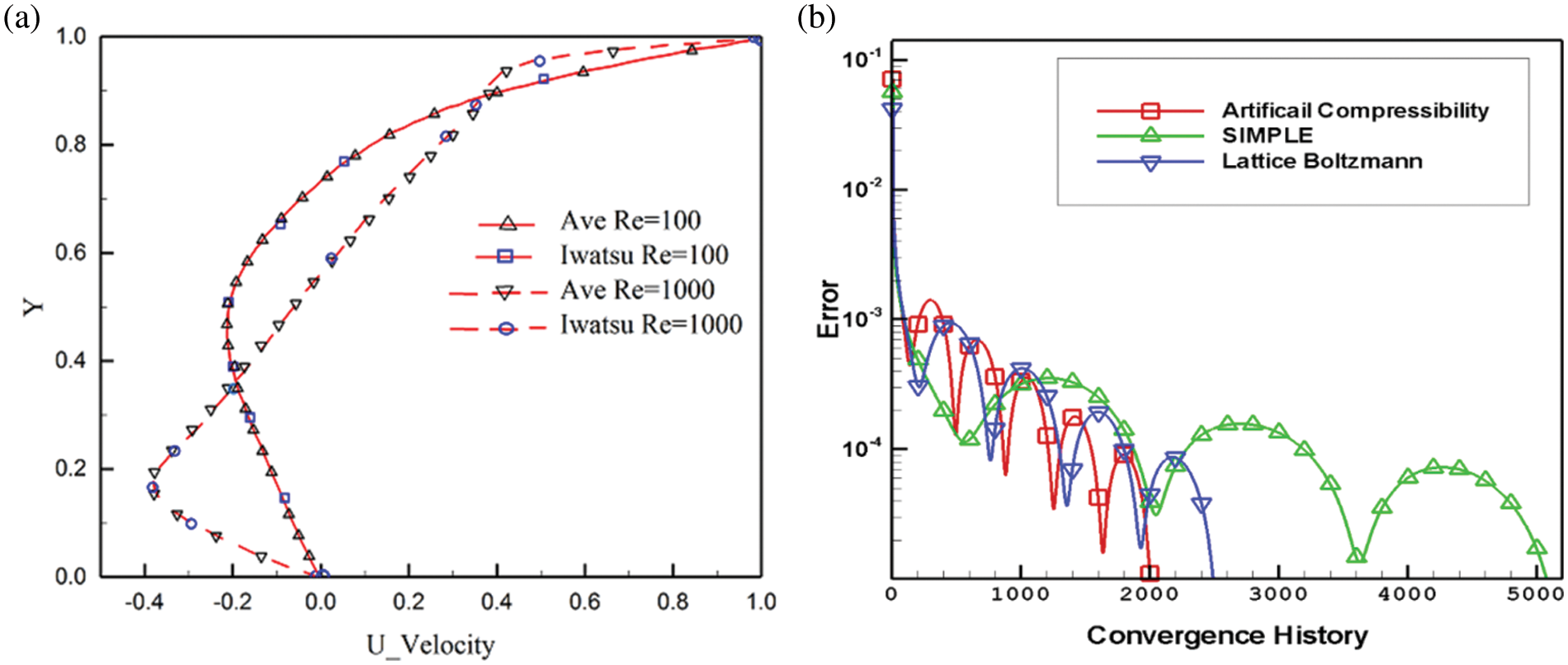
Figure 4: a) Comparison of present and Iwatsu’s [63] results in terms of the velocity on the vertical centerline of the cavity, b) Comparison of convergence speed of three different schemes

One of the well-known problems of viscous flow is the flow inside a square cavity. Depending on the Reynolds number, one or more vortices have been formed inside the cavity. As the Reynolds number increases, the number of vortices increases. The incompressible and viscous steady flow inside the cavity is a well-known example of a case test used to validate a novel numerical scheme. The simple and the clustered quadrilateral grid have been used in this work. The natural and mixed convection nanofluid flows are considered in this paper. First, natural convection (Gr = 0) is considered and then mixed convections with non-zero Grashof numbers are simulated. In the first case, the continuity and momentum equations are solved simultaneously and the velocity and pressure fields are determined. By placing the velocity and pressure fields in the energy equation, the temperature field is determined. Nevertheless, in mixed convection, the momentum equation is a function of Grashof number and temperature. Therefore, all the equations should be solved simultaneously to determine the pressure, velocity and temperature fields. In numerical techniques, the Courant number is taken into account and is defined as follows:

C=uΔtΔx(19)

Courant number is a factor used to determine the convergence of the numerical method. Convergence speed improves as the Courant number is increased. However, the numerical method diverges with higher Courant numbers. Mathematical approaches can be used to determine the range of courant numbers required for convergence in simpler cases with simple governing equations. Nevertheless, in more complex equations, this range is determined by numerical experiments. To find this range, the written code for the numerical scheme is run for different Courant numbers until the code output diverges and the highest achievable value for Courant numbers is determined. Convergence history for various Courant numbers with β=5 is derived and displayed in Fig. 5a. As seen in Fig. 5a, increasing the courant number speeds up convergence. The simulation has been run for different artificial compressibility factors (0.1, 1, 5, and 20) at a constant Courant number and the results are depicted in Fig. 5b. The convergence speed is seen to be high for small artificial compressibility factors. For each artificial compressibility factor, the simulation has been repeated to the maximum Courant number (Fig. 5b). The results indicate that there is no substantial difference in the rate of convergence.

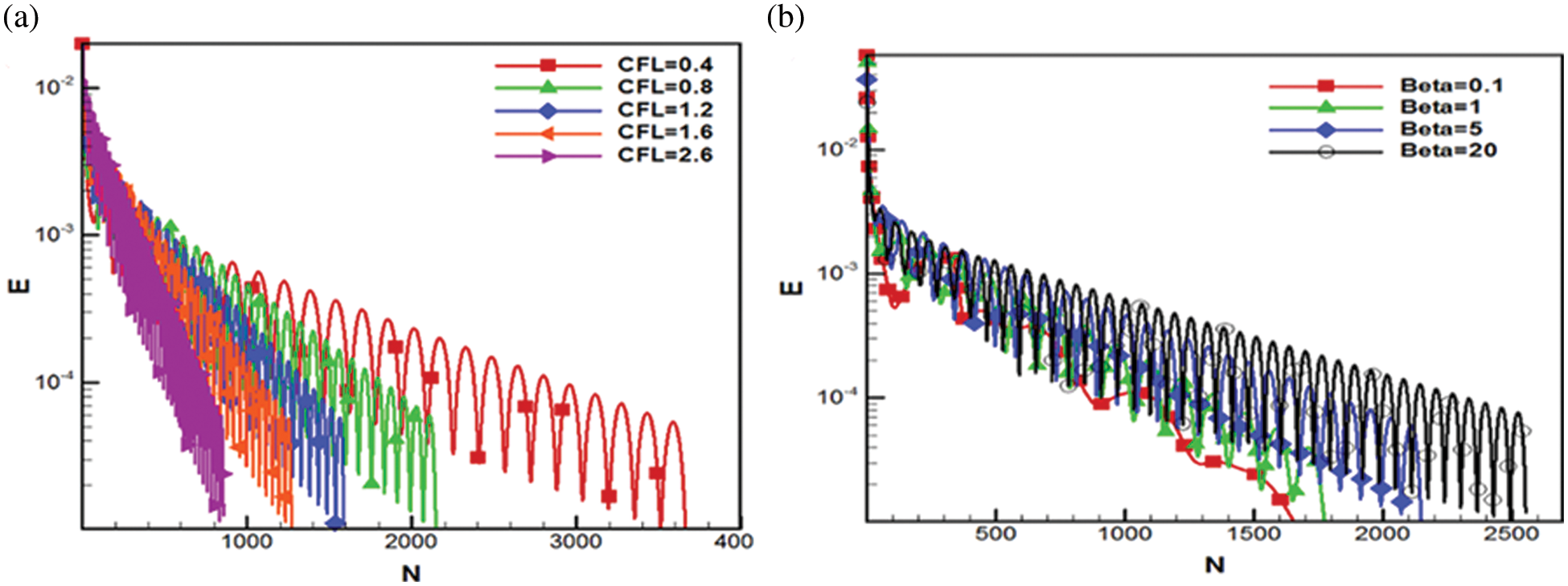
Figure 5: a) Convergence history for various artificial compressibility factor (Gr = 0, Re = 100, Pr = 6.161), b) Convergence history for different artificial compressibility factors and maximum possible Courant number (Gr = 0, Re = 100, Pr = 6.161)

To assess the effect of the artificial compressibility coefficient on the results, the friction coefficients at the bottom plate are calculated and compared for various artificial compressibility coefficients, as illustrated in Fig. 6a. In the figure, the coefficient of friction gradually increases for the bottom plate and the page, changes behavior and the coefficient of friction decreases. As seen in Fig. 6a, the compression ratio has no effect on the physical outcomes. This is because this coefficient appears as a pressure-time gradient coefficient in the continuity relation. Because these problems are steady and have a steady-state solution, the pressure gradient with respect to time is zero, and the artificial compressibility coefficient impact is eliminated during the last step of numerical solutions. Additionally, the equations for unsteady flows are utilized to obtain the numerical solution for steady-state flows. In other words, the pseudo time marching is done on unsteady equations to reach a solution for steady-state flow problems. This approach begins with an arbitrary initial condition for the numerical solution of the equations and determines the solutions in each step based on the preceding step data. The temperature variation along the horizontal centerlines of the cavity is obtained by numerical solution of the energy equation. Obtained temperature is shown in Fig. 6b at different artificial compressible factors. The results show that obtained temperature is the function of the artificial compressibility coefficient. In other words, the results show that the effect of the artificial compressibility coefficient has not been completely eliminated in the final step of numerical simulation. This implies that the results are converged in such a way that the pressure gradient coefficient is not zero in the final steps of the numerical solution.

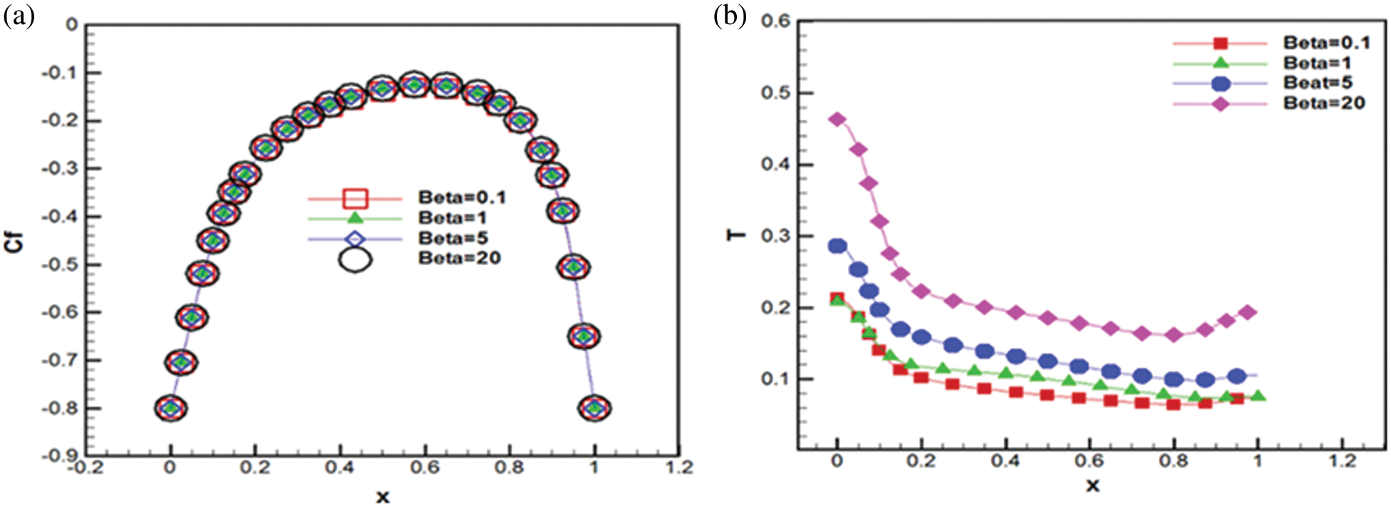
Figure 6: a) Friction coefficient variation at the top plate with different artificial compressibility (Gr = 0, Re = 100, Pr = 6.16), b) Temperature variation in the horizontal centerline of the cavity with different artificial compressibility factors (Gr = 0, Re = 100, Pr = 6.161)

It is noted that the deviation from the results occurs when the artificial compressibility coefficient is changed abruptly. With 200 times the artificial compressibility coefficient, the resulting change is observed (Fig. 6b). Therefore, researchers who use the artificial compression method for numerical simulations must first eliminate the artificial compressibility factor effect on the results before proceeding with other simulations. In the other words, the simulation must be performed using different artificial compressibility factors, and once the effect of the compressibility factor is eliminated from the results, the subsequent simulations must use this artificial compressibility factor. An artificial compressibility factor of 1 to 5 can be a good start for simulations, according to the results shown in Fig. 6b.

The governing equations are numerically solved, and velocity, pressure and temperature fields are obtained. The resulting temperature field is used to display the isotherms (Fig. 7) using the “Tecplot” software. Fig. 7 demonstrates that the isotherms are perpendicular to the left and right walls. This is because the left and right walls are insulated. In addition, the magnitude of the artificial compressibility factor shows a minimal effect on isotherms. Mixed convection with a high Grashof number is simulated in this step. The momentum equation is a function of the Grashof number and the governing equations are solved simultaneously. The pressure, velocity and temperature fields are obtained by solving the governing equations. The convergence history for different artificial compressibility factors is observed and shown in Fig. 8a. Convergence speed is found slower when the artificial compressibility factor is low (0.1) or high (20). Therefore, the fastest convergence occurs for the artificial compressibility factors of 1 to 5. The results of temperature changes are analyzed in different directions. Fig. 8b shows the temperature variation along the horizontal centerline that passes through the center of the cavity with different β. Temperature changes along the screen are decreased and the majority of changes are associated with beta = 20, with the exception of divergence at beta = 20. To survey the obtained results in Fig. 8b, the simulations are conducted with a grid of 6400 cells and the results are shown in Fig. 9a. As seen in the figure, the temperature variations are not the same, which is not due to the number of cells used in the computational domain. These differences are mainly because of the artificial compressibility term. This term does not tend to zero in some cases, according to the results. The Nusselt number variation is illustrated in Fig. 9b for the top and bottom walls. Except for β=1, the figure reveal that the Nusselt number variation is independent of the artificial compressibility factor.

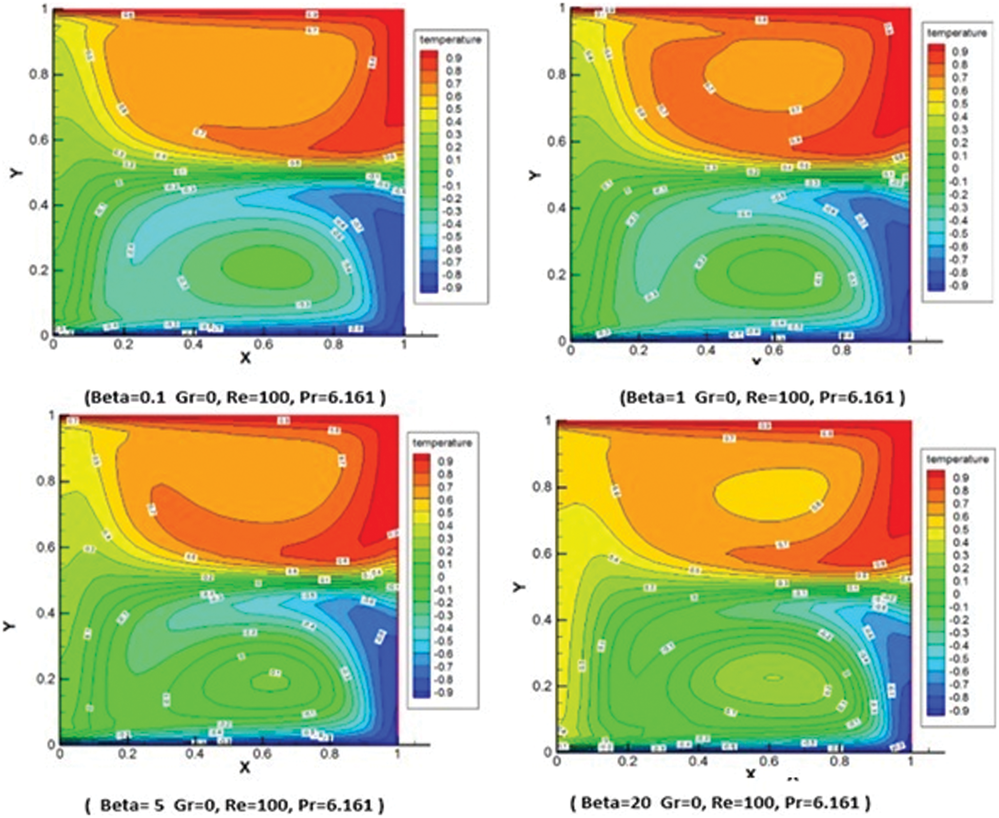
Figure 7: Isotherms with different artificial compressibility factors (Gr = 0, Re = 100, Pr = 6.161)

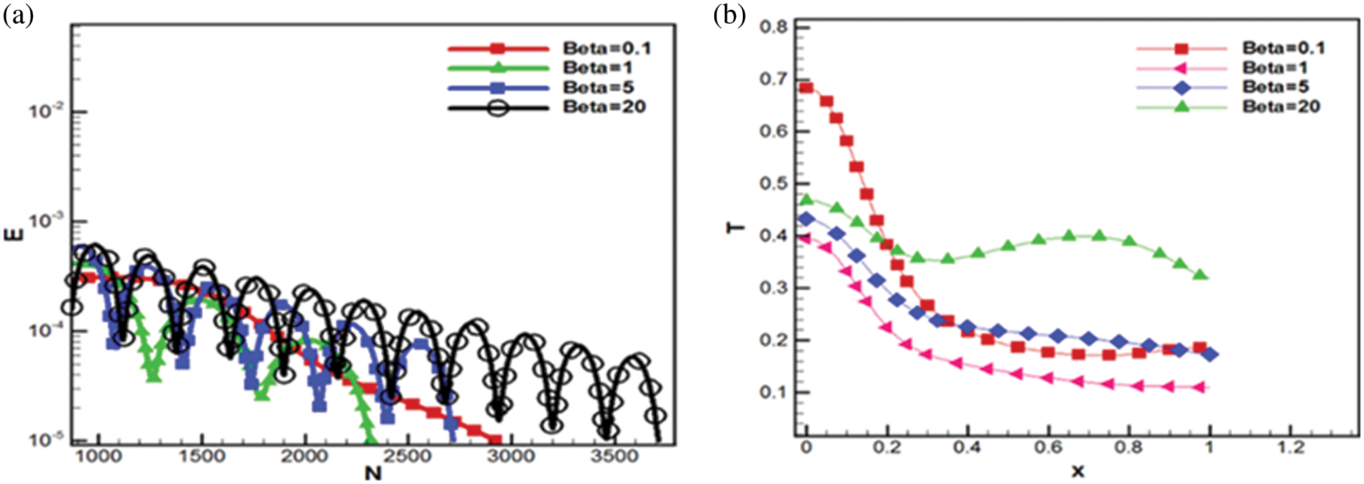
Figure 8: a) Convergence history for different artificial compressibility factors (Re = 20, Gr = 40, Pr = 6.161), b) Temperature variation along the horizontal centerline of the cavity with different artificial compressibility factors (Re = 20, Gr = 40, Pr = 6.161)

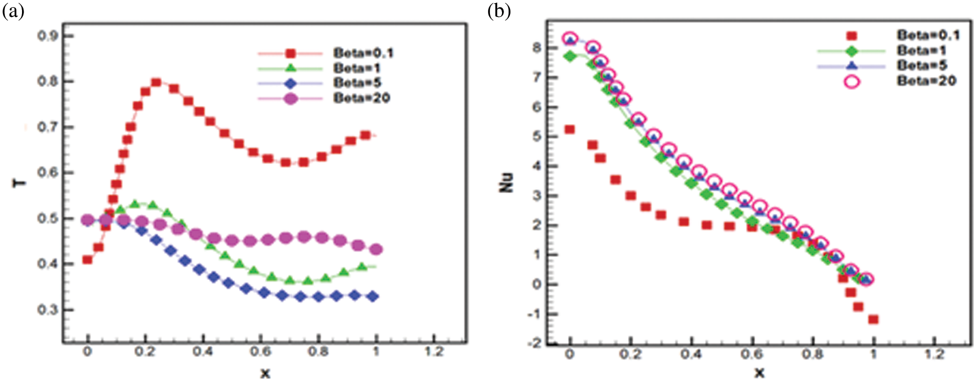
Figure 9: a) Temperature variation along the horizontal centerline of the cavity with different artificial compressibility factors with 6400 cells (Re = 20, Gr = 40, Pr = 6.161) b) Nusselt number variation on the top wall for different artificial compressibility factor (Re = 20, Gr = 40, Pr = 6.161)

5  Conclusion

In this study, a numerical simulation of a two-dimensional incompressible flow with heat transfer inside a square cavity was investigated using an artificial compressibility method. The effect of the artificial compressibility coefficient on convergence speed and accuracy of results was also assessed. It is found that the accuracy of the results is affected if the artificial compression ratio is either too small or too large. In other words, the artificial compressibility term may not tend to zero at the final steps of time marching. The results also demonstrated that the optimal values of the artificial compressibility factor lie between 1 and 5 for viscous incompressible flows. Using the artificial compressibility method necessitates a measure comparable to network independence, as indicated by the results. In other words, simulations should initially be conducted with varying values of the synthetic compressibility factor, and if the results do not change, simulations should continue. By determining the optimal number for the artificial compressibility factor, researchers in the field of numerical techniques can ensure the speed of convergence as well as the accuracy of the results. This study employed the fifth-order Rung-Kutta method in conjunction with the artificial compressibility method. Simulations could utilize more numerical approaches. The convective fluxes are obtained using the method of averaging. The characteristics-based method could be used.

Funding Statement: The authors extend their appreciation to the Deanship of Scientific Research at King Khalid University for funding this work through the Large Groups Project under grant number RGP. 2/235/43.

Conflicts of Interest: The authors declare that they have no conflicts of interest to report regarding the present study.

References

1. Z. Peng, E. Doroodchi and B. Moghtaderi, “Heat transfer modelling in Discrete Element Method (DEM)-based simulations of thermal processes: Theory and model development,” Progress in Energy and Combustion Science, vol. 79, pp. 100–107, 2020. [Google Scholar]
2. M. M. Ali, R. Akhter and M. Alim, “Performance of flow and heat transfer analysis of mixed convection in Casson fluid filled lid driven cavity including solid obstacle with magnetic impact,” SN Applied Sciences, vol. 3, no. 2, pp. 1–15, 2021. [Google Scholar]
3. H. Wang, H. Wang, F. Gao, P. Zhou and Z. J. Zhai, “Literature review on pressure–velocity decoupling algorithms applied to built-environment CFD simulation,” Building and Environment, vol. 143, pp. 671–678, 2018. [Google Scholar]
4. D. Kwak, C. Kiris and C. S. Kim, “Computational challenges of viscous incompressible flows,” Computers & Fluids, vol. 34, no. 3, pp. 283–299, 2005. [Google Scholar]
5. V. Kornilov, “Current state and prospects of researches on the control of turbulent boundary layer by air blowing,” Progress in Aerospace Sciences, vol. 76, pp. 1–23, 2015. [Google Scholar]
6. T. C. Corke and F. O. Thomas, “Dynamic stall in pitching airfoils: Aerodynamic damping and compressibility effects,” Annual Review of Fluid Mechanics, vol. 47, pp. 479–505, 2015. [Google Scholar]
7. J. Qin, H. Pan, M. M. Rahman, X. Tian and Z. Zhu, “Introducing compressibility with SIMPLE algorithm,” Mathematics and Computers in Simulation, vol. 180, pp. 328–353, 2021. [Google Scholar]
8. D. Ntouras and G. Papadakis, “A coupled artificial compressibility method for free surface flows,” Journal of Marine Science and Engineering, vol. 8, no. 8, pp. 1–12, 2020. [Google Scholar]
9. J. Manzanero, G. Rubio, D. A. Kopriva, E. Ferrer and E. Valero, “An entropy–stable discontinuous Galerkin approximation for the incompressible Navier–Stokes equations with variable density and artificial compressibility,” Journal of Computational Physics, vol. 408, pp. 109–121, 2020. [Google Scholar]
10. M. M. Mousa, M. R. Ali and W. -X. Ma, “A combined method for simulating MHD convection in square cavities through localized heating by method of line and penalty-artificial compressibility,” Journal of Taibah University for Science, vol. 15, no. 1, pp. 208–217, 2021. [Google Scholar]
11. N. Jiang, Y. Li and H. Yang, “An artificial compressibility Crank--Nicolson leap-frog method for the Stokes--Darcy model and application in ensemble simulations,” SIAM Journal on Numerical Analysis, vol. 59, no. 1, pp. 401–428, 2021. [Google Scholar]
12. K. Nagata, N. Ikegaya and J. Tanimoto, “Consideration of artificial compressibility for explicit computational fluid dynamics simulation,” Journal of Computational Physics, vol. 443, pp. 110–125, 2021. [Google Scholar]
13. D. Dupuy, A. Toutant and F. Bataille, “Analysis of artificial pressure equations in numerical simulations of a turbulent channel flow,” Journal of Computational Physics, vol. 411, pp. 109–121, 2020. [Google Scholar]
14. J. -K. Zhang, M. Cui, B. -W. Li and Y. -S. Sun, “Performance of combined spectral collocation method and artificial compressibility method for 3D incompressible fluid flow and heat transfer,” International Journal of Numerical Methods for Heat & Fluid Flow, vol. 30, no. 12, pp. 5037–5062, 2020. [Google Scholar]
15. W. Zhong, A. Yu, X. Liu, Z. Tong and H. Zhang, “Dem/CFD-DEM modelling of non-spherical particulate systems: Theoretical developments and applications,” Powder Technology, vol. 302, pp. 108–152, 2016. [Google Scholar]
16. T. Adibi and S. E. Razavi, “A new characteristic approach for incompressible thermo-flow in Cartesian and non-Cartesian grids,” International Journal for Numerical Methods in Fluids, vol. 79, no. 8, pp. 371–393, 2015. [Google Scholar]
17. S. E. Razavi and T. Adibi, “A novel multidimensional characteristic modeling of incompressible convective heat transfer,” Journal of Applied Fluid Mechanics, vol. 9, no. 4, pp. 1135–1146, 2016. [Google Scholar]
18. J. Marti and P. Ryzhakov, “Improving accuracy of the moving grid particle finite element method via a scheme based on Strang splitting,” Computer Methods in Applied Mechanics and Engineering, vol. 369, pp. 113–121, 2020. [Google Scholar]
19. N. K. Goona, S. R. Parne and S. Sashidhar, “Distributed source scheme to solve the classical form of Poisson equation using 3-D finite-difference method for improved accuracy and unrestricted source position,” Mathematics and Computers in Simulation, vol. 190, pp. 965–975, 2021. [Google Scholar]
20. A. Baeza, R. Bürger, P. Mulet and D. Zorío, “An efficient third-order WENO scheme with unconditionally optimal accuracy,” SIAM Journal on Scientific Computing, vol. 42, no. 2, pp. 1028–1051, 2020. [Google Scholar]
21. Z. Shah, E. O. Alzahrani, A. Dawar, A. Ullah and I. Khan, “Influence of Cattaneo-Christov model on Darcy-Forchheimer flow of micropolar ferrofluid over a stretching/shrinking sheet,” International Communications in Heat and Mass Transfer, vol. 110, pp. 104–119, 2020. [Google Scholar]
22. A. M. Mahdy, M. Babatin and M. Khader, “Numerical treatment for processing the effect of convective thermal condition and Joule heating on Casson fluid flow past a stretching sheet,” International Journal of Modern Physics C, pp. 225–232, 2022. [Google Scholar]
23. P. Lin and A. Ghaffari, “Steady flow and heat transfer of the power-law fluid between two stretchable rotating disks with non-uniform heat source/sink,” Journal of Thermal Analysis and Calorimetry, vol. 146, no. 4, pp. 1735–1749, 2021. [Google Scholar]
24. S. El-Sapa, M. S. Mohamed, K. Lotfy, A. Mahdy and A. El-Bary, “Photo-elasto-thermodiffusion waves of fractional heat order excited with laser short-pulse impact for semiconductor medium,” Journal of Low Temperature Physics, pp. 1–20, 2022. [Google Scholar]
25. M. Bhatti, A. Ghaffari and M. Doranehgard, “The role of radiation and bioconvection as an external agent to control the temperature and motion of fluid over the radially spinning circular surface: A theoretical analysis via Chebyshev spectral approach,” Mathematical Methods in the Applied Sciences, pp. 1–13, 2022. [Google Scholar]
26. M. Khader, N. Swetlam and A. Mahdy, “The Chebyshev collection method for solving fractional order Klein-Gordon equation,” WSEAS Transactions on Mathematics, vol. 13, pp. 2224–2880, 2014. [Google Scholar]
27. A. Mahdy, “A numerical method for solving the nonlinear equations of Emden-Fowler models,” Journal of Ocean Engineering and Science, pp. 1–12, 2022. [Google Scholar]
28. A. Mahdy and E. Youssef, “Numerical solution technique for solving isoperimetric variational problems,” International Journal of Modern Physics C, vol. 32, no. 1, pp. 215–222, 2021. [Google Scholar]
29. A. M. Mahdy, “Numerical solutions for solving model time-fractional Fokker–Planck equation,” Numerical Methods for Partial Differential Equations, vol. 37, no. 2, pp. 1120–1135, 2021. [Google Scholar]
30. A. M. Mahdy, Y. A. E. Amer, M. S. Mohamed and E. Sobhy, “General fractional financial models of awareness with Caputo–Fabrizio derivative,” Advances in Mechanical Engineering, vol. 12, no. 11, pp. 1–12, 2020. [Google Scholar]
31. A. Mahdy, “Numerical studies for solving fractional integro-differential equations,” Journal of Ocean Engineering and Science, vol. 3, no. 2, pp. 127–132, 2018. [Google Scholar]
32. N. H. Sweilam, M. M. Khader and A. M. Mahdy, “Numerical studies for fractional-order logistic differential equation with two different delays,” Journal of Applied Mathematics, vol. 20, pp. 12–22, 2012. [Google Scholar]
33. G. M. Ismail, A. Mahdy, Y. Amer and E. Youssef, “Computational simulations for solving nonlinear composite oscillation fractional,” Journal of Ocean Engineering and Science, pp. 1–14, 2022. [Google Scholar]
34. T. Gul, S. Nasir, S. Islam, Z. Shah and M. A. Khan, “Effective Prandtl number model influences on the γAl2O3-H2O and γAl2O3-C2H6O2 nanofluids spray along a stretching cylinder,” Arabian Journal for Science & Engineering (Springer Science & Business Media BV), vol. 44, no. 2, pp. 23–28, 2019. [Google Scholar]
35. M. Ijaz Khan, Usman, A. Ghaffari, S. Ullah Khan, Y. -M. Chu and S. Qayyum, “Optimized frame work for Reiner–Philippoff nanofluid with improved thermal sources and Cattaneo–Christov modifications: A numerical thermal analysis,” International Journal of Modern Physics B, vol. 35, no. 6, pp. 215–222, 2021. [Google Scholar]
36. A. S. Khan, Y. Nie, Z. Shah, A. Dawar, W. Khan et al., “Three-dimensional nanofluid flow with heat and mass transfer analysis over a linear stretching surface with convective boundary conditions,” Applied Sciences, vol. 8, no. 11, pp. 22–34, 2018. [Google Scholar]
37. Y. -M. Li, “Numerical simulations for three-dimensional rotating porous disk flow of viscoelastic nanomaterial with activation energy, heat generation and Nield boundary conditions,” Waves in Random and Complex Media, pp. 1–20, 2022. [Google Scholar]
38. Z. Shah, A. Tassaddiq, S. Islam, A. Alklaibi and I. Khan, “Cattaneo–Christov heat flux model for three-dimensional rotating flow of SWCNT and MWCNT nanofluid with Darcy–Forchheimer porous medium induced by a linearly stretchable surface,” Symmetry, vol. 11, no. 3, pp. 320–331, 2019. [Google Scholar]
39. M. Shamshuddin, A. Ghaffari and Usman, “Radiative heat energy exploration on Casson-type nanoliquid induced by a convectively heated porous plate in conjunction with thermophoresis and Brownian movements,” International Journal of Ambient Energy, pp. 1–12, 2021. [Google Scholar]
40. T. Adibi, S. E. Razavi, O. Adibi, M. Vajdi and F. S. Moghanlou, “The response of nano-ceramic doped fluids in heat convection models: A characteristics-based numerical approach,” Scientia Iranica, vol. 28, no. 5, pp. 2671–2683, 2021. [Google Scholar]
41. Z. Shah, E. O. Alzahrani, W. Alghamdi and M. Z. Ullah, “Influences of electrical MHD and Hall current on squeezing nanofluid flow inside rotating porous plates with viscous and joule dissipation effects,” Journal of Thermal Analysis and Calorimetry, vol. 140, no. 3, pp. 1215–1227, 2020. [Google Scholar]
42. A. Dawar, S. Islam, A. Alshehri, E. Bonyah and Z. Shah, “Heat transfer analysis of the MHD stagnation point flow of a non-Newtonian tangent hyperbolic hybrid nanofluid past a non-isothermal flat plate with thermal radiation effect,” Journal of Nanomaterials, vol. 20, pp. 1–12, 2022. [Google Scholar]
43. S. Muhammad, G. Ali, Z. Shah, S. Islam and S. A. Hussain, “The rotating flow of magneto hydrodynamic carbon nanotubes over a stretching sheet with the impact of non-linear thermal radiation and heat generation/absorption,” Applied Sciences, vol. 8, no. 4, pp. 48–62, 2018. [Google Scholar]
44. A. Mahdy, K. Lotfy, E. Ismail, A. El-Bary, M. Ahmed et al., “Analytical solutions of time-fractional heat order for a magneto-photothermal semiconductor medium with Thomson effects and initial stress,” Results in Physics, vol. 18, pp. 103–114, 2020. [Google Scholar]
45. A. Mahdy, K. Lotfy, A. El-Bary and H. Sarhan, “Effect of rotation and magnetic field on a numerical-refined heat conduction in a semiconductor medium during photo-excitation processes,” The European Physical Journal Plus, vol. 136, no. 5, pp. 1–17, 2021. [Google Scholar]
46. A. Mahdy, K. Lotfy, A. El-Bary and I. M. Tayel, “Variable thermal conductivity and hyperbolic two-temperature theory during magneto-photothermal theory of semiconductor induced by laser pulses,” The European Physical Journal Plus, vol. 136, no. 6, pp. 1–21, 2021. [Google Scholar]
47. N. Sweilam, M. Khader and A. Mahdy, “Computional methods for fractional differential equations generated by optimization problem,” Journal of Fractional Calculus and Applications, vol. 3, pp. 1–12, 2012. [Google Scholar]
48. A. M. Mahdy, M. Higazy and M. S. Mohamed, “Optimal and memristor-based control of a nonlinear fractional tumor-immune model,” Materials & Continua, vol. 67, no. 3, pp. 3463–3486, 2021. [Google Scholar]
49. A. Mahdy, K. Lotfy and A. El-Bary, “Use of optimal control in studying the dynamical behaviors of fractional financial awareness models,” Soft Computing, vol. 26, no. 7, pp. 3401–3409, 2022. [Google Scholar]
50. K. Gepreel, M. Higazy and A. Mahdy, “Optimal control, signal flow graph and system electronic circuit realization for nonlinear Anopheles mosquito model,” International Journal of Modern Physics C, vol. 31, no. 9, pp. 205–218, 2020. [Google Scholar]
51. H. Alotaibi, K. A. Gepreel, M. S. Mohamed and A. M. Mahdy, “An approximate numerical methods for mathematical and physical studies for covid-19 models,"Computer Systems Science and Engineering, vol. 42, no. 3, pp. 1147–1163, 2022. [Google Scholar]
52. A. Mahdy, K. Gepreel, K. Lotfy and A. El-Bary, “A numerical method for solving the Rubella ailment disease model,” International Journal of Modern Physics C, vol. 32, no. 7, pp. 215–222, 2021. [Google Scholar]
53. A. Mahdy, M. Mohamed, K. Lotfy, M. Alhazmi, A. El-Bary et al., “Numerical solution and dynamical behaviors for solving fractional nonlinear Rubella ailment disease model,” Results in Physics, vol. 24, pp. 104–21, 2021. [Google Scholar]
54. K. Gepreel, A. Mahdy, M. Mohamed and A. Al-Amiri, “Reduced differential transform method for solving nonlinear biomathematics models,” Computers, Materials and Continua, vol. 61, no. 3, pp. 979–994, 2019. [Google Scholar]
55. A. Mahdy and M. Higazy, “Numerical different methods for solving the nonlinear biochemical reaction model,” International Journal of Applied and Computational Mathematics, vol. 5, no. 6, pp. 1–17, 2019. [Google Scholar]
56. S. El-Sapa, K. Gepreel, K. Lotfy, A. El-Bary and A. Mahdy, “Impact of variable thermal conductivity of thermal-plasma-mechanical waves on rotational microelongated excited semiconductor,” Journal of Low Temperature Physics, pp. 1–22, 2022. [Google Scholar]
57. G. M. Ismail, K. Gepreel, K. Lotfy, A. Mahdy, A. El-Bary et al., “Influence of variable thermal conductivity on thermal-plasma-elastic waves of excited microelongated semiconductor,” Alexandria Engineering Journal, vol. 61, no. 12, pp. 12271–12282, 2022. [Google Scholar]
58. M. Mohamed, K. Lotfy, A. El-Bary and A. Mahdy, “Photo-thermal-elastic waves of excitation microstretch semiconductor medium under the impact of rotation and initial stress,” Optical and Quantum Electronics, vol. 54, no. 4, pp. 1–21, 2022. [Google Scholar]
59. A. K. Khamis, K. Lotfy, A. El-Bary, A. M. Mahdy and M. Ahmed, “Thermal-piezoelectric problem of a semiconductor medium during photo-thermal excitation,” Waves in Random and Complex Media, vol. 31, no. 6, pp. 2499–2513, 2021. [Google Scholar]
60. A. Mahdy, K. Lotfy and A. El-Bary, “Thermo-optical-mechanical excited waves of functionally graded semiconductor material with hyperbolic two-temperature,” The European Physical Journal Plus, vol. 137, no. 1, pp. 1–17, 2022. [Google Scholar]
61. M. Mohamed, K. Lotfy, A. El-Bary and A. Mahdy, “Absorption illumination of a 2D rotator semi-infinite thermoelastic medium using a modified Green and Lindsay model,” Case Studies in Thermal Engineering, vol. 26, pp. 101–165, 2021. [Google Scholar]
62. S. E. Razavi, T. Adibi and S. Faramarzi, “Impact of inclined and perforated baffles on the laminar thermo-flow behavior in rectangular channels,” SN Applied Sciences, vol. 2, no. 2, pp. 284–294, 2020. [Google Scholar]
63. R. Iwatsu, J. M. Hyun and K. Kuwahara, “Mixed convection in a driven cavity with a stable vertical temperature gradient,” International Journal of Heat and Mass Transfer, vol. 36, no. 6, pp. 1601–1608, 1993. [Google Scholar]
Cite This Article
Copyright © 2023 The Author(s). Published by Tech Science Press.
This work is licensed under a Creative Commons Attribution 4.0 International License , which permits unrestricted use, distribution, and reproduction in any medium, provided the original work is properly cited.
Downloads
Citation Tools