A More Efficient Approach for Remote Sensing Image Classification

1  Introduction

SSC via ML algorithms is an active research area in RSI data analysis. In fact, the critical step in almost all computer vision tasks is developing discriminative features to represent visual data [1–6]. In the past decades, the classical ML-SSC methods proposed in previous studies can be roughly divided into three categories according to the different feature extraction approaches, i.e., handcrafted features [7], unsupervised learning features [8], and DL features [9,10]. Driven by the advances in big data, hardware computing resources, and iterative algorithms, the DL-based algorithm has rapidly overwhelmed the RSI-SSC research area in the past decade, accounting for the advantage in many aspects, such as classification accuracy, fully automatic feature learning and representation, and generalization ability. As the algorithm’s engine, a series of DL models have been proposed, e.g., deep belief networks [11], auto-encoders [12], generative adversarial networks [13], and deep CNNs [14]. In the last five years, the deep CNN has gradually become prominent in the RSI-SSC research fields, mainly owing to its end-to-end feature learning and higher classification accuracy.

Training a deep CNN model from scratch commonly requires massive amounts of annotated data. However, it is hard to obtain such a large RSI dataset without a big research team. Hence, transfer learning approaches based on pre-trained models of natural images have been the prior mainstream route, which mainly includes fine-tuning models [15] and using models as feature extractors with frozen architecture parameters [16]. Under this situation, no overwhelming advantages were found until those large-scale RSI datasets of SSC benchmarks appeared, i.e., the AID [17] and NWPU-RESISC45D [18]. Since then, many CNN-based RSI-SSC approaches have been demonstrated successively.

Firstly, those approaches by using classic CNN models as feature extractors coupled with feature fusion, feature re-weighting, or feature recombination strategies were proposed. Chaib et al. [19] employed a pre-trained visual geometry group network (VGGNet) as a deep feature extractor and then fused those every-layer features after a discriminant correlation analysis (DCA). The results were finally treated as final representations for RSI-SSC. Wang et al. [20] also employed a pre-trained Alex CNN (AlexNet) as a deep feature extractor, but differently added a long-short-term memory network into the algorithm as the attention weight matrix generator. Then they re-weighted the 5th layer output features of the AlexNet with the attention weight matrixes and fed the results to an attention recurrent convolutional network (ARCNet) for RSI-SSC. These two approaches both show an overwhelming performance against those traditional ML methods, but the performance evaluation by the OA on AID is still less than 93%. Moreover, as a preliminary exploration, Cheng et al. [21] separately employed three pre-trained CNN models, i.e., an AlexNet, a VGGNet, and a Google CNN (GoogleNet) as deep feature extractors, and then re-combined the deep features as image descriptors for the input of a bag of convolutional features (BoCF) model. In the end, the output of the BoCF model was fed into a linear support vector machine classifier for RSI-SSC. Unsurprisingly, the approach’s OA on NWPU-RESISC45D is a very limited 84.32%.

These three previous works are all rough or coarse applications of deep CNN. The model’s under-fitting state, coming from poor training and unwise reprocessing of deep features, has greatly decreased the model’s performance. To improve classification accuracy, approaches based on CNN models as feature extractors coupled with re-mined information of interclass relationships were presented. Liu et al. [22] leveraged three pre-trained CNN models, i.e., an AlexNet, a VGGNet-16, and a VGGNet-Places365 as multi-scale deep feature extractors, and then re-used those extracted features as source data to obtain the ground Wasserstein distance (WD) matrix. At the end of the approach’s pipeline, they engineered a handcrafted WD loss instead of the routine cross-entropy loss and retrained a GoogleNet model for RSI-SSC. Furthermore, Liu et al. [23] re-used the same WD idea again and fused the multi-information extracted from three retrained CNN models, i.e., an AlexNet, a VGGNet-16, and a GoogleNet, for building sample class category hierarchies of RSI. After being re-weighted by the hierarchical results, the hierarchical WD (HWD) loss was purposely embedded into the training process of individual CNN models for RSI-SSC. Similarly, Zhang et al. [24] also employed two pre-trained CNN models (i.e., a VGGNet-16 and an Inception-V3) as feature extractors and then fed deep features into a capsule network (CapsNet) for the purpose of achieving a better capture of the spatial and hierarchical information of RSI. Sorting these three approaches’ OAs, the WD-CNN is at the best 97.24% on AID, while the HWD-CNN is at the best 94.38% on NWPU-RESISC45D.

Despite the complex process and so many handcrafted features, these three prior approaches do lift the performance of CNNs in RSI-SSC noticeably. Hence, more approaches utilizing the spatial attention mechanism or the combination of multi-level deep features, as well as the ensemble of multi-CNNs, have been demonstrated and shown to have more competitive OAs than ever. Zhu et al. [25] sought to obtain deep features and spatial attention maps, respectively, based on a residual CNN (ResNet) and a gradient-weighted class activation mapping technique. Then those attention maps were fed into a designed spatial feature transformer network to generate saliency map features, which were successively fused with the CNN features by dot multiplication. In the end, an attention-based deep feature fusion (ADFF) CNN model was built for RSI-SSC. Similarly, Zhu et al. [26] employed a Caffe CNN to extract deep features and simultaneously engineered an adaptive deep sparse semantic modeling (ADSSM) framework to extract mid-level features. Then the mid-level features were fused with high-level ones for RSI-SSC. Differently, Minetto et al. [27] employed a dozen ResNets and dense CNNs to build a CNN ensemble called “Hydra”, which includes two CNNs in the body and twelve CNNs in the heads. The output score of each head of Hydra was involved in a majority vote in which a negative result represents the number of votes below or equal to half the sum of heads. Amid the three approaches’ OAs, only the ADFF-CNN tested on AID is at 94.75%, which is below the WD-CNN. But when comparing OAs on NWPU-RESISC45D, the Hydra ensemble is at best 94.51%.

However, the significant advantage of DL is end-to-end automatic feature learning with little expert experience dependence. Furthermore, the trade-off of a DL-based approach is always important owing to the fixed hardware budget, particularly the graphics processing unit (GPU) budget. Back to the aforementioned representative studies, we can find that these approaches are full of either multi-stages or excessive parameters (i.e., corresponding with out-of-control trade-offs), as well as too many handcrafted features or discriminators (i.e., corresponding with high expert experience dependence). In our options, automation and simplicity are the top priorities of the DL algorithm, i.e., it is unnecessary to sacrifice them for the excessive pursuit of accuracy.

Generally speaking, manually labeling a massive dataset is time-consuming. Hence, data augmentation is routinely employed at training time in DL tasks to improve model generalization and reduce over-fitting [28–30]. Moreover, other data preprocessing techniques recently introduced for natural image classification have also shown advantages in potentially improving model validation accuracy, robustness, and convergence speed simultaneously, with more significant gains in training efficiency. In other words, efficiency optimization has become an indispensable part of the training process of deep neural networks. However, to the best of our knowledge, we find that these very meaningful techniques have not been applied sufficiently in the earlier CNN-based studies. Despite this, the backbone CNN models used in the previous studies are former SOTA models, and more efficient ones have recently been demonstrated.

Therefore, we believe that this situation may have caused three problems. Firstly, the earlier approaches may have achieved suboptimal performances considering the lack of efficiency optimization in the training process. Secondly, the earlier performance evaluation results of CNN-based algorithms for RSI-SSC may be inaccurate somehow owing to the lack of efficient training. Thirdly, and most crucially, it will be very likely to achieve a new SOTA performance for RSI-SSC while the priorities of simplicity and automation are retained if the latest model and efficient optimization in the training process are reasonably employed.

Motivated by the above questions, in this study we propose a fast and simple training CNN framework named FST-EfficientNet for RSI-SSC. More specifically, we introduce a set of classical data preprocessing techniques both for training and testing efficiency optimization into a CNN model, i.e., the EfficientNetV2-S [31], but still employ a typical and simple transfer learning strategy. During the practice of the FST-EfficientNet, we only employ several routine data augmentation tricks coupled with a fixed ratio of resolution or a gradually increasing resolution strategy to speed up the convergence rate and improve the model’s performance. The whole process of the proposed algorithm is completely one-stage and end-to-end, without any handcrafted features or discriminators involved. The three contributions of this study are summarized as follows:

Firstly, our FST-EfficientNet achieved new SOTA performance records for AID and NWPU-RESISC45D challenges via a routine transfer learning strategy. The model has fewer parameters at about 22 mega (M) with 8.8 billion (B) floating point operations (FLOPs), and the whole algorithm flowchart is understandable.

Secondly, our FST-EfficientNet practice demonstrates the importance and indispensability of training efficiency optimization strategies in RSI-SSC by DL. The techniques can significantly boost model performance and reduce time costs as well in RSI-SSC tasks.

Thirdly, and most crucially, the results of our study suggest that it is unwise to give up simplicity and automation unthinkingly in RSI-SSC tasks by DL. We argue that an excellent DL-based algorithm should include simplicity and automation as much as possible. To address this, we must pay more attention to the new techniques emerging in the natural image classification domain, particularly when developing new CNN-based methods.

2  Materials and Methods

2.1 Model Architecture

The framework of FST-EfficientNet is illustrated in Fig. 1. On the top of Fig. 1, we can observe the flowchart of the FST-EfficientNet and the base model’s architecture, i.e., the original EfficientNetV2-S, which includes stage0–7 blocks and one pooling and full-connection (FC) linear classifier layer. More specifically, stage0 and stage7 have fewer conv-layers inside compared to other stages, i.e., stage0 includes only one down-sample 3 × 3 conv-layer with a 2 × 2 stride, while stage7 includes only one 1 × 1 conv-layer with a 1 × 1 stride. However, the stage 1–6 blocks are composed of multi-conv-layers that are called the Mobilenet conv-layer (MBC) [32] or Fused Mobilenet conv-layer (FMBC) [33]. In detail, the number of FMBCs in stages 1–3 is 2, 4, and 4, while the number of MBCs in stages 4–6 is 6, 9, and 15. Inside the framework of the FST-EfficientNet, we only fine-tune the linear classifier layer of the original EfficientNetV2-S architecture, i.e., the model’s original parameters and FLOPs are unchanged.

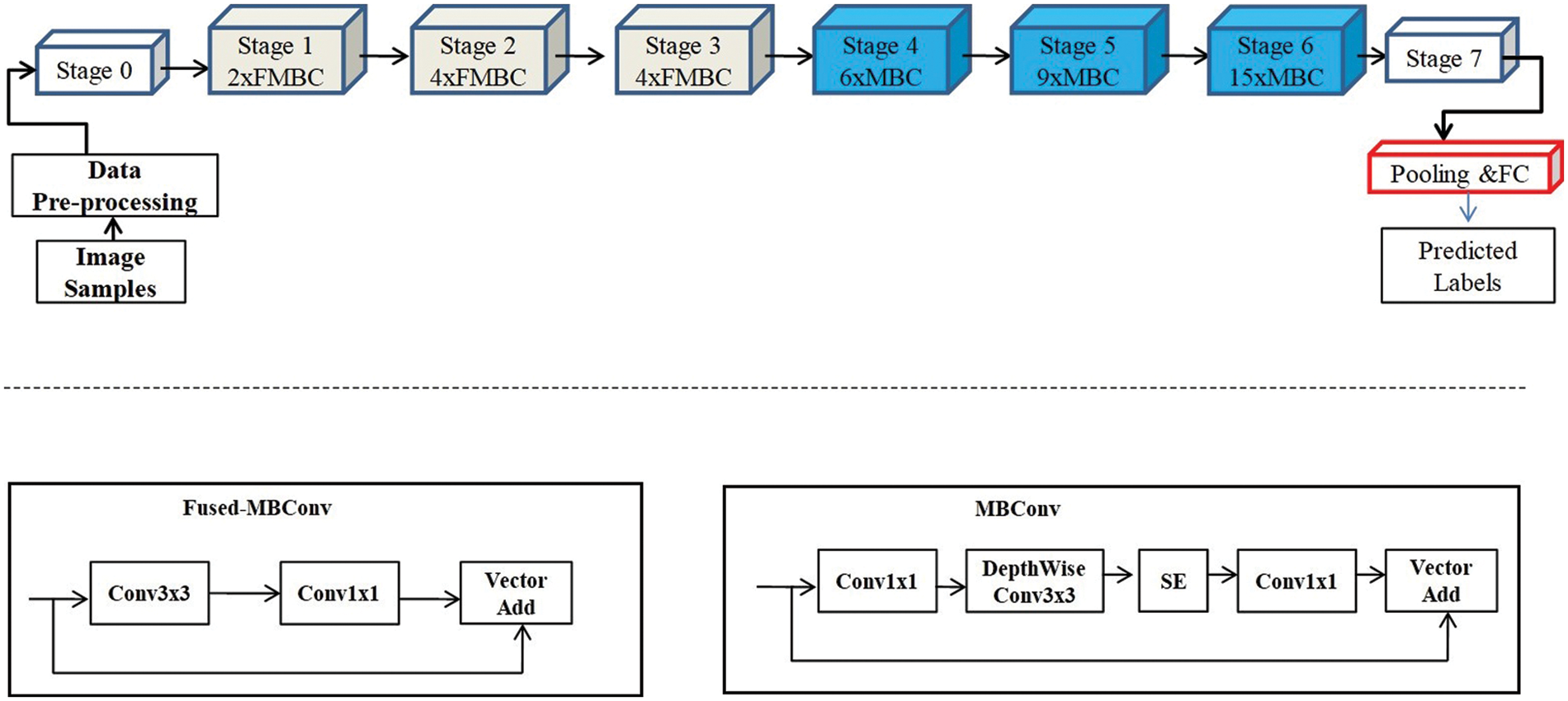
Figure 1: The framework of FST-EfficientNet and structure changes between the MBC and FMBC

The EfficientNetV2 CNN family models were released by Tan et al. in 2021. The model architecture is developed by using a combination of training-aware neural architecture search and scaling. The largest one of the family models holds a new SOTA top-1 accuracy of 87.3% on ImageNet-2012. The EfficientNetV2 architecture is an improvement on the previous EfficientNet [34], which was released in 2019. In terms of parameters and FLOPs, the EfficientNet architecture was smaller and faster at that time. But as Radosavovic et al. [35] concluded in 2020, the size of the output tensors of all conv-layers, which is defined as “activations”, can heavily affect the run-time on memory-bound hardware accelerators, i.e., GPU accelerators. That is, the higher total number of activations and convolution operations of the EfficientNet architecture slows down the training and inference speeds in practice.

To solve the problems, several changes were made to the EfficientNetV2 architecture design. As shown at the bottom of Fig. 1, the most significant change in conv-layer structure is the MBC replaced by the FMBC, i.e., the structure of a depth-wise 3 × 3 conv-layer behind the expansion 1 × 1 conv-layer, which is also called the depth-wise separable convolution, is replaced by a single regular conv3 × 3. Secondly, the Squeeze-and-Excitation (SE) block, which improves CNN performance via the channel attention mechanism, is excluded from the FMBC. It is well known that the SE block has two conv-layers. Understandably, these two changes in structure will greatly reduce the conv-layer activations and convolution operations. Additionally, a non-uniform scaling strategy is used for different stages in EfficientNetV2, compared to the same scaling rule for all stages in EfficientNet. Eventually, the baseline model with 8 stages, which is named “EfficientNetV2-S”, is developed with 22 M parameters and 8.8B FLOPs.

The EfficientNetV2-S model not only achieves better classification accuracy on Image-Net2012 with smaller parameters and FLOPs, but also has good transfer learning performance on other datasets. In addition, the model’s source code is publicly available on the internet for nearly unlimited usage. Therefore, the EfficientNetV2-S model is employed in this study for research purposes owing to its smaller size and better performance.

2.2 Dataset

There are two RSI datasets used in this study, i.e., AID and NWPU-RESISC45D. The AID was released in 2017 with a total of 30 scene subclasses and 10,000 images, while each subclass contains 220–420 images at a fixed resolution of 600 × 600 pixels. The images are cropped from Google Earth images and the spatial resolution is about 0.5–8 m. The samples for each category are shown in Fig. 2. Similarly, the NWPU-RESISC45D was published in 2017 with a total of 45 subclasses and 31,500 images, while each class contains 700 images at a fixed resolution of 256 × 256 pixels. The images are also cropped from Google Earth images and the spatial resolution is about 0.2–30 m. The samples for each category are shown in Fig. 3.

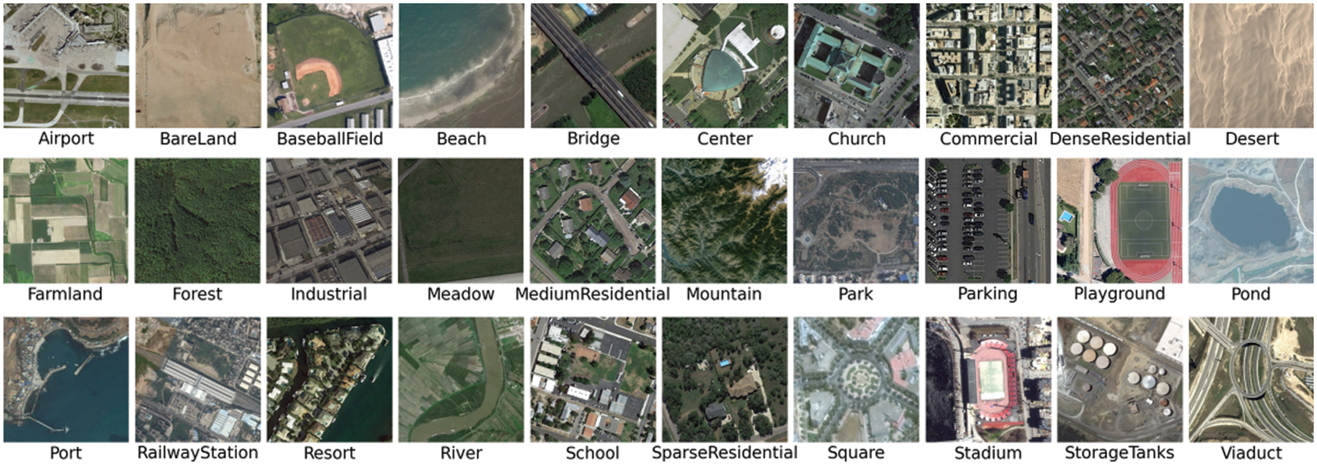
Figure 2: Sample images of AID for 30 subclasses

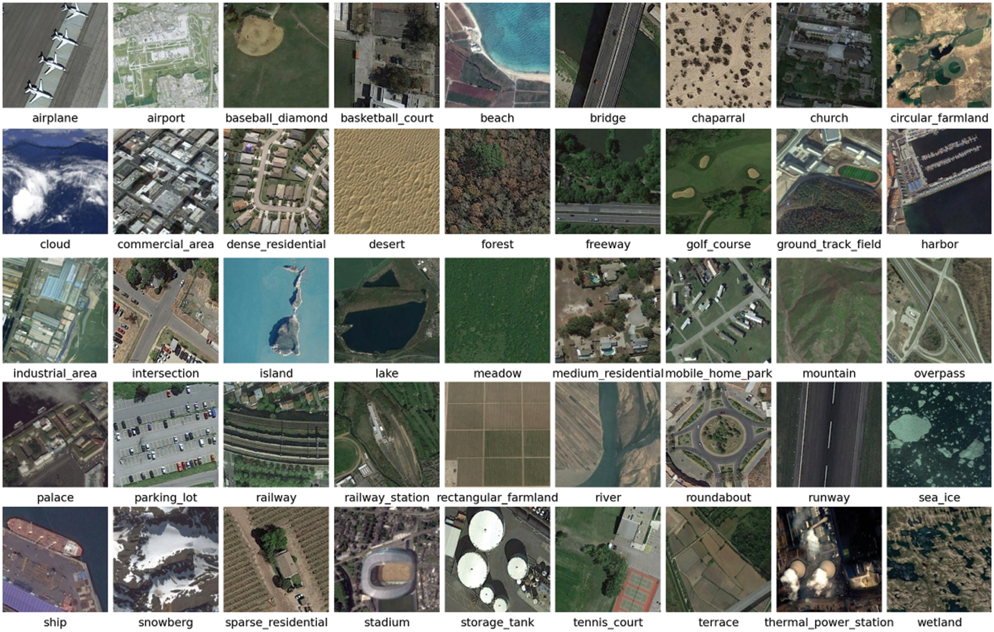
Figure 3: Sample images of NWPU-RESISC45D for 45 subclasses

These two datasets have been commonly used as benchmarks in previous studies. In brief, the OA and confusion matrix have been widely used as evaluation criteria for the approaches’ performance. In detail, the OA is as described in Eq. (1):

OA=Nc/Nt(1)

where the OA is defined as the total number of accurately classified samples (Nc) divided by the total number of tested samples (Nt).

The confusion matrix is a detailed classification result table of the performance belonging to every single classifier; i.e., for each element Xij (i represents lines and j represents rows) in the table, the proportion of the predicted images in the ith category that actually belong to the jth class is computed.

In addition, for algorithm performance evaluation, a typically fixed training ratio of these two datasets has been widely used, with the remaining for testing. In detail, training ratios of 20% and 50% have been used for AID, while training ratios of 10% and 20% have been used for NWPU-RESISC45D. For a fair comparison, the evaluation criterion and training ratio in this study are the same.

2.3 Proposed Approach

2.3.1 Related Work

Training efficiency has become more and more important with the continuous expansion of deep learning applications, and recently, many techniques have been demonstrated to either shorten training time or improve model performance.

Initially, Howard [36] demonstrated a “progressive resizing” method by using smaller images at the start of training and gradually increasing image size at further training steps. To be specific, the typical 224 × 224 resolution of the Imagenet-2012 dataset used in training time is replaced by a 128 × 128 resolution at initial epochs, and then larger size images (a resolution of 288 × 288, etc.) are used at the final epochs. However, the testing accuracy is not very ideal, though the convergence speed has improved. Furthermore, Hoffer et al. [37] proposed a “Mix & Match” (MM) method by using stochastic images and batch sizes through random sampling to improve the training and inference speed. The study shows that the CNN model accuracy, as well as robustness to image scale variants, can be improved, and the total number of training iterations can also be reduced. For the same purpose, Tan et al. also proposed a new method called “progressive learning” (PL) when EfficientNetV2 was released. In detail, the study demonstrates a similar progressive strategy by increasing the image size at training time but differently by using a stronger regularization at training time as the image size increases, which is called “adaptive regularization.” The study also shows that the PL technique can improve the accuracy and reduce the training time of EfficientNetV2 synchronously, and the technique can also work well for EfficientNet and ResNet. However, the MM and PL techniques are designed and applied for training CNNs from scratch on super-large-scale datasets, which are 100 to 400 times bigger than the RSI ones.

Finally, Touvron et al. [38] proposed another “FixRes” method. In detail, at the initial training steps, the strategy of a fixed ratio of image resolution, which includes a smaller image sampled by the random-size crop (RSC) transformation (i.e., cropping a random portion of the original image and resizing it to a given size) for training but a larger image for testing, is employed. But in the final training steps, as the training images change to larger ones, another strategy by fine-tuning the model’s last several layers or making some parametric adaptations to the activation of the model’s pooling layer is employed to gain non-trivial performance improvements. Since the paper’s publication, the FixRes technique has been widely examined on a lot of SOTA CNN models, and the latest result shows that the FixRes is a model-agnostic technique with simple and cheap parameter adaptations [39]. More specifically, the training strategy via FixRes is 2.3 times faster than the routine ones, with understandably cheaper trade-offs owing to the smaller training image size consuming less GPU memory while it works well in transfer learning. However, these very meaningful techniques have never been applied in RSI-SSC ever. There may be a great chance to improve the CNN-based algorithm’s performance in RSI-SSC tasks if these simple techniques are properly used.

Therefore, in the study, we employ a partial idea of the FixRes technique in our FST-EfficientNet. Similarly, we use the RSC transformation and set a fixed training vs. testing resolution ratio at the initial training steps, and then change the RSC to the resize transformation for the same larger resolution both in the training and testing process during the later training steps. Differently, at the final training steps, we just train the model normally instead of fine-tuning layers or making parametric adaptations introduced by FixRes, mainly considering that the RSI datasets are smaller than natural image ones. For the same reason, in the base EfficientNetV2-S model, we also keep the dropout rate before the linear classifier layer and other stochastic-depth settings as default. The increasing image resolution is separately used in our FST-EfficientNet with respective results compared to the sequential one in the PL method. In other words, the whole idea of the MM method is not implemented in our study yet.

2.3.2 Algorithm

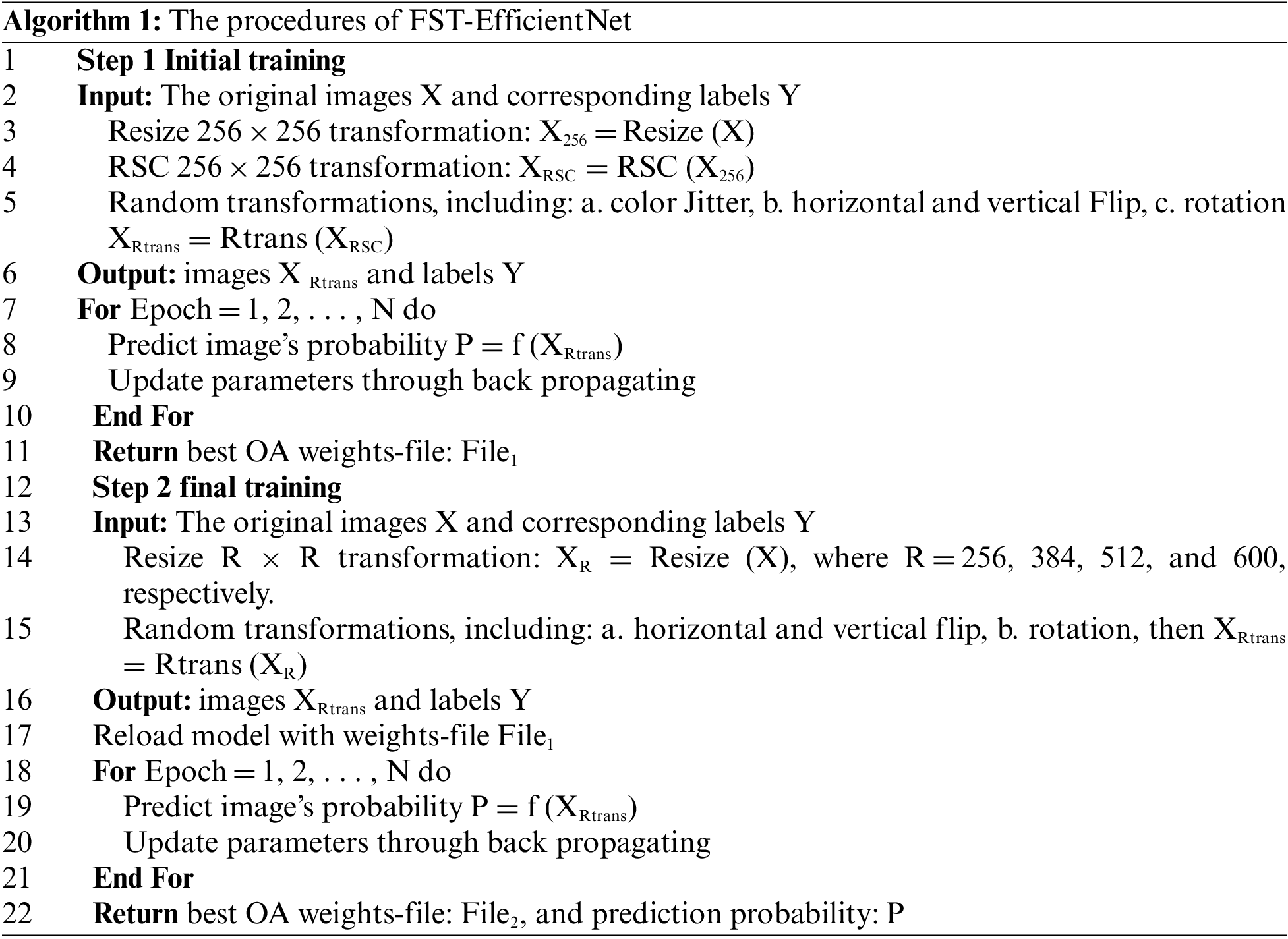
Algorithm 1 summarizes the running process of the FST-EfficientNet framework. In summary, the approach can be divided into Steps 1 and 2 according to the different resolutions used for training and testing. In detail, Step 1 includes a total training epoch of 120, an initial learning rate of 0.001 with cosine decay, a training image resolution of 208 × 208, a testing image resolution of 256 × 256, and a training batch size of 36 with all transformations used. More specifically, all layers of the model are frozen except the classifier during the initial training epochs of 20, and then all layers are unfrozen during the remaining training epochs of 100. Correspondingly, Step 2 includes a total training epoch of 240, an initial learning rate of 0.0001 with cosine decay, training and testing images with the same resolutions of 256 × 256–512 × 512 for NWPU-RESISC45D (but 256 × 256–600 × 600 for AID), and a training batch size of 24 to 36 for NWPU-RESISC45D (but 18 to 36 for AID) with all transformations used except the RSC. All layers of the model are unfrozen during all the training epochs of 240. In addition, in training, the loss function is the cross-entropy loss function, and the error back propagation algorithm is the stochastic gradient descent with a momentum of 0.9 and a weight decay of 0.0001. The EfficientNetV2-S model is initialized by the “rwightman” pre-trained weights-file on ImageNet2012 [40].

2.3.3 Data Augmentation and Dataset Division

We employ six kinds of image transformations to implement data augmentation during training, i.e., the RSC, resize, color jitter, random rotation, random horizontal, and vertical flip transformation. The running order of transformations is the resize followed by the RSC, and then is the color jitter, horizontal flip, vertical flip, and rotation in turn. Only the resize transformation is applied to images during testing. In our implementation, the sequentially transformed images are generated on the central processing unit (CPU) via the default Python code in the PyTorch libraries while the GPU is training on the previous batch of transformed images. As a result, these data augmentation schemes do not increase any GPU’s trade-off.

In general, all the experiments in this study were conducted by using a random selection of images in each subclass from the dataset, and the results of OA were averaged over three runs.

2.3.4 Hardware and Software Environments

The experiments were performed on a personal computer equipped with an AMD Ryzen 5700X CPU, a single RTX2060 GPU with 12 gigabytes (GB) of video random access memory (RAM), and 32 GB of RAM, running Pytorch 1.11.0 with the Compute Unified Device Architecture (CUDA) 11.5 on Win 10.

3  Results

3.1 OA on AID

Table 1 reports the OA comparison of different methods on AID with a training ratio of 20% and 50%. Given the description in Table 1, the OA results of the line Step 1 are related to a training size of 208 × 208 (by the RSC transformation) and a testing size of 256 × 256, compared to a fixed training and testing size of 600 × 600 for the line Step 2. Given the results of the previous studies in Table 1, our FST-EfficientNet is outperforming all the other methods noticeably. For example, the CapsNet claims the highest OA of 93.79% with a training ratio of 20% before 2021, which is some 1.00% lower than our result of step 1 and, more significantly, some 2.58% lower than the result of step 2, respectively. Similarly, the WD claims the highest OA of 97.24% by the training ratio of 50%, which is still some 0.77% lower than the result of step 2, although a very lower testing ratio of 30% is used in the WD method. If comparing our FST-EfficientNet to those earlier methods, e.g., the DCA, ARCNet, and ADFF, we can observe a greater OA gap.

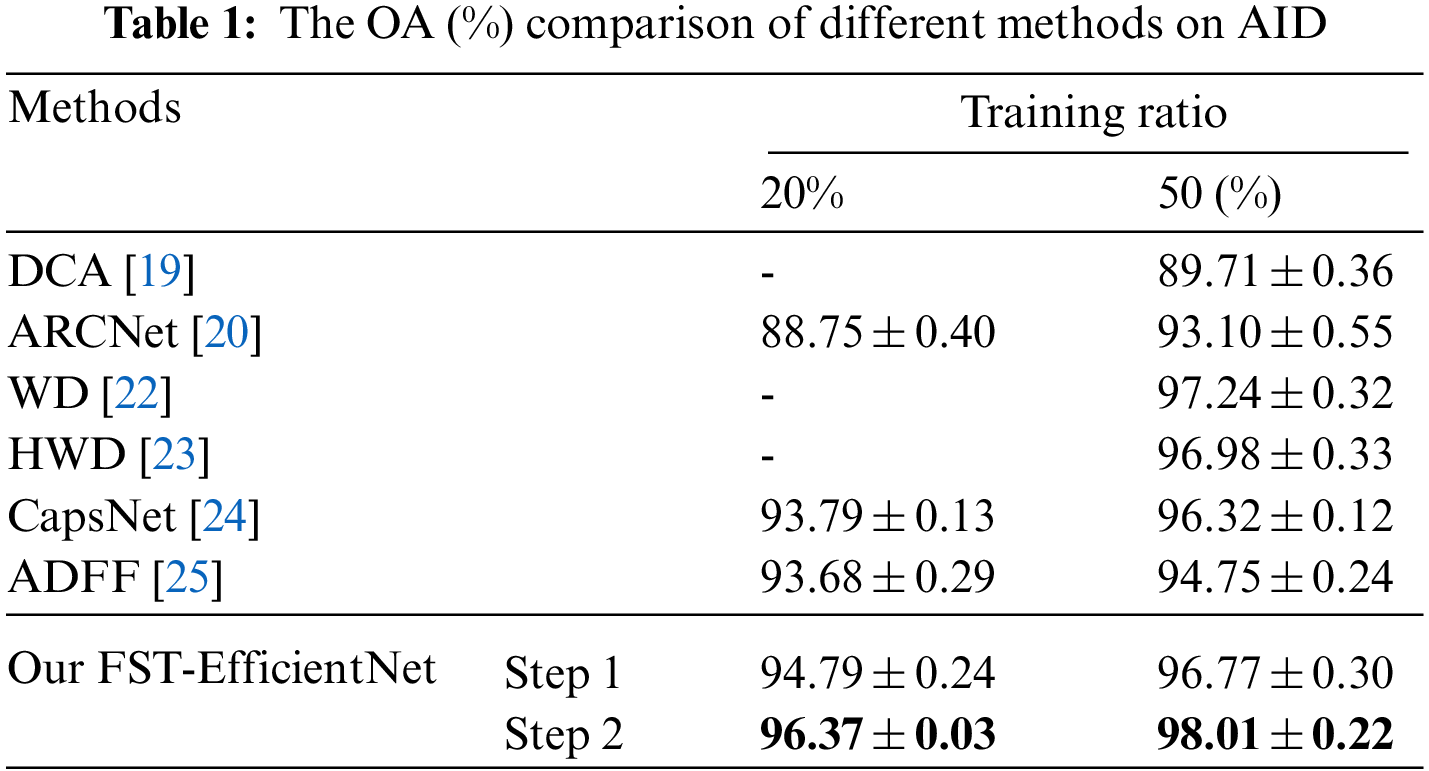
Regardless of the OA’s difference, these six methods both have a common complexity and require prior expert experience. Additionally, the handcrafted features and indicators that do exist in these methods may have decreased the model’s generalization ability, i.e., these methods may be over-fitting on AID owing to the huge parameters corresponding to handcrafted engineering.

Hence, our FST-EfficientNet does present excellent performance on the relatively small AID, with better simplicity, automation, and generalization ability considering its transfer learning strategy.

3.2 Confusion Matrix of AID

Fig. 4 presents the confusion matrixes of AID at a resolution of 600 × 600. As shown in Fig. 4a, 26 of all the 30 scene subclasses gain classification OAs higher than 90%, and five subclasses, including “beach”, “forest”, “mountain”, “port”, and “viaduct”, achieve OAs of 100%. Only 3 of these 26 subclasses, including “industrial”, “medium residential”, and “square”, gain OAs lower than 96.37%, indicating that only 7 of all the 30 scene subclasses have relatively greater interclass dissimilarities in AID. In addition, the subclasses with lower OAs, including “center”, “park”, “resort” and “school”, are also consistent with the CapsNet, but the OAs of the three subclasses in our study are higher by 2.8%, 6.5% and 12.9%, respectively. As shown in Fig. 4b, the confusion mainly happens in the “center”, “park”, “resort”, and “school” scenes. The results are roughly aligned when considering that in Fig. 4a, but the OA of the “center” scene shows a 12.1% increase in Fig. 4b.

Figure 4: Confusion matrixes of AID at a resolution of 600 × 600

In brief, the results do show that our approach significantly improves the classification accuracy. However, for the several subclasses with greater interclass dissimilarity, i.e., “center”, “park”, “resort”, “square” and “school” scenes, there is still a need for more training samples to gain better performance.

3.3 OA on NWPU-RESISC45D

Table 2 presents the OA comparison of different methods on NWPU-RESISC45D with a training ratio of 10% and 20%. Given the description in Table 2, the OA results of the line Step 1 are the same as the setting in Table 1, but instead of a different setting by a fixed size of 512 × 512 for the line Step 2. Given the results of earlier studies in Table 2, our FST-EfficientNet is still outperforming noticeably. For example, the HWD claims a high OA of 93.27% (by a training ratio of 20% but a different testing ratio of 30%) in 2018, which is some 1.43% lower than the result of Step 1 and some 2.33% lower than the result of Step 2, respectively. Similarly, the ADSSM claims a high OA of 91.69% (by a training ratio of 10%) and 94.29% (by a training ratio of 20%), which is about 0.4%–0.7% lower than the result of Step 1 and 1.3%–2.0% lower than the result of Step 2, respectively. More specifically, the OA results of Step 2 show a 1.3% increase (by a training ratio of 10%) and a 1.1% increase (by a training ratio of 20%) compared to the Hydra, which claims the highest OA of 92.44% and 94.51%.

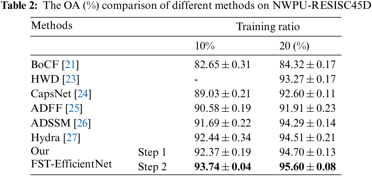
Combining the information in Tables 1 and 2, the results suggest that our FST-EfficientNet has shown consistently outperforming performance against the other methods, even if the total number of samples increases 3 times from AID to NWPU-RESISC45D. Compared to the fourteen CNN models accumulated in the Hydra method, our FST-EfficientNet is also a good explanation that it is not necessary to gain better classification accuracy in RSI-SSC based on the excessive trade-off.

3.4 Confusion Matrix of NWPU-RESISC45D

Fig. 5 displays the confusion matrixes of NWPU-RESISC45D at a resolution of 512 × 512. As shown in Fig. 5a, 38 of all the 45 scene subclasses gain classification OAs higher than 90%, and only the “chaparral” subclass achieves the OA of 100%. The confusion mainly happens in “church” and “palace” scenes with OAs lower than 85% and also happens in “commercial area”, “dense residential”, “railway station”, and “wet land” scenes with OAs close to 90%. Given the results shown in Fig. 5b, only two subclasses gain OAs lower than 90%, i.e., the “church” and “palace” scenes, meaning there is a need for more training samples to improve the model’s performance. The CapsNet study argues that the similar styles of buildings in the “church” and “palace” scenes contribute to the classification confusion. However, the ADSSM method shows a significant improvement in the classification OA of the “church” scene in contrast to more suboptimal performance in the other scenes (i.e., “storage tank”, “basketball court”, “tennis court”, “overpass”, etc.), indicating that there is a chance to improve the CNN-based classification accuracy on NWPU-RESISC45D. Nevertheless, the results do show that our approach significantly improves classification accuracy on NWPU-RESISC45D in general.

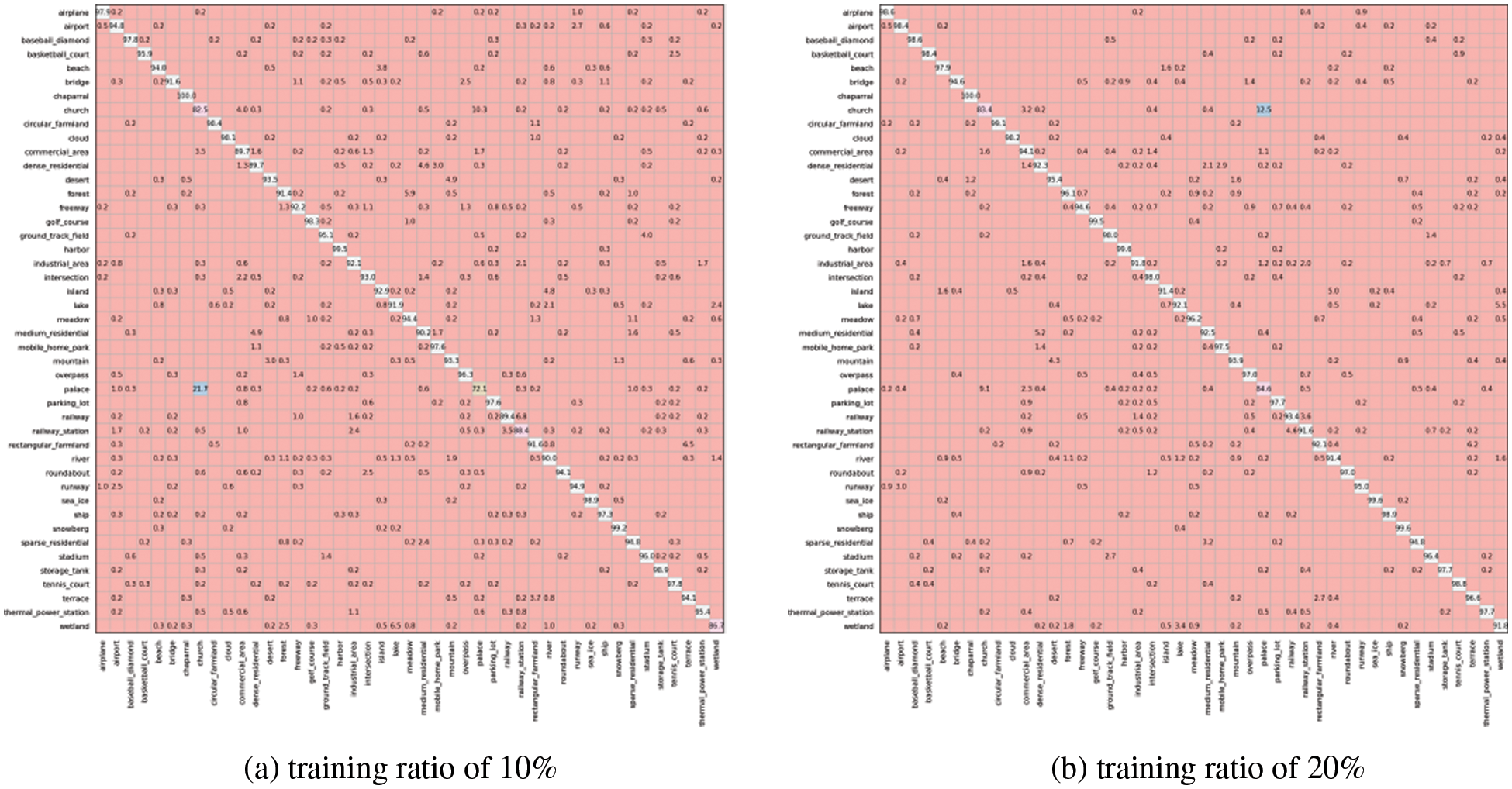
Figure 5: Confusion matrixes of NWPU-RESISC45D at a resolution of 512×512

4  Discussions

Training and testing with larger image sizes for the CNN model always leads to a higher OA. To examine the optimum resolution for classification, we also changed the image size of Step 2 on the two datasets, i.e., AID from 256 × 256 to 600 × 600 and NWPU-RESISC45D from 256 × 256 to 512 × 512, both in the training and testing period respectively, with other experimental settings unchanged. Table 3 presents the OA results. The larger resolution of 600 × 600 leads to a significant 0.8% increase on AID compared to 256 × 256. Similarly, the larger resolution of 512 × 512 leads to a significant 0.5% increase on NWPU-RESISC45D. More specifically, the improvement is more evident in the lower train ratio. Considering the consumption of GPU resources and time-cost, the method’s efficiency in practice may be better at the resolution of 384 × 384.

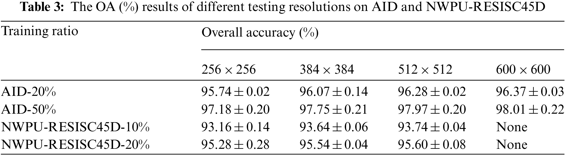
This result does demonstrate that using a larger image size for the CNN-based method can lead to a higher OA for RSI-SSC. However, if using larger images at a “one-size-fits-all” resolution as previous studies do, the memory consumption of GPUs will go up, and the model’s speed in training and testing will be reduced more. In other words, the traditional methods in previous studies have higher time and hardware costs, which restrict the use of larger image sizes for achieving better model performance. Hence, the data preprocessing strategy used in this study offers us a new route to boost model performance with a limited cost for RSI-SSC.

Nevertheless, there are still some limitations in our study to date. Firstly, only the channel attention mechanism is included in the model architecture via SE blocks, and it is well known that the spatial attention mechanism can boost model performance simultaneously. Secondly, transformed images via RSC have a random size for training input, so the convergence rate may fluctuate more than usual. Thirdly, the initial learning rate of 0.001 at Step 1 may be too high for the transfer learning strategy, so the present results may be suboptimal somehow. We will check all these similar questions in the future.

5  Conclusions

RSI-SSC via CNN-base DL method is a rapidly developing research field, and many academics have made massive efforts to seek better performance during the past decade. However, some of these prior studies unwisely pay more unbalanced attention to the classification accuracy than the algorithm’s efficiency.

In this study, we propose the FST-EfficientNet, which is a fast and simple training CNN framework for RSI-SSC. The whole algorithm flow is completely one-stage and end-to-end without any handcrafted features or discriminators involved. In the implementation of training efficiency optimization, only some routine tricks run on the CPU, so the algorithm’s trade-off is very cheap. The performances on the two datasets (i.e., AID and NWPURESISC45D) show that the OA results are new SOTA records with about 0.8% to 2.7% ahead of all earlier methods, to our best knowledge. Meanwhile, our study demonstrates the importance and indispensability of the training efficiency optimization strategy for RSI-SSC by DL. It is not necessary to gain better classification accuracy in RSI-SSC based on the excessive trade-off. In the end, we hope these findings can help the development of more efficient CNN-based approaches for RSI-SSC in the future.

Acknowledgement: Thanks to Meta AI Research for Pytorch. Thanks to Tan and Le for EfficientNetV2. Thanks to Xia et al. for the AID. Thanks to Cheng et al. for the NWPU-RESISC45D. Thanks to all the anonymous reviewers for their helpful suggestions.

Funding Statement: This research has been supported by Doctoral Research funding from Hunan University of Arts and Science, Grant Number E07016033.

Conflicts of Interest: The author declares that he has no conflicts of interest to report regarding the present study.

References

1. A. Althobaiti, A. Alhumaidi Alotaibi, S. Abdel-Khalek, S. A. Alsuhibany and R. F. Mansour, “Intelligent deep data analytics based remote sensing scene classification model,” Computers, Materials & Continua, vol. 72, no. 1, pp. 1921–1938, 2022. [Google Scholar]
2. J. Escorcia-Gutierrez, M. Gamarra, M. Torres-Torres, N. Madera, J. C. Calabria-Sarmiento et al., “Intelligent sine cosine optimization with deep transfer learning based crops type classification using hyperspectral images,” Canadian Journal of Remote Sensing, 2022. [Online]. Available: https://doi.org/10.1080/07038992.2022.2081538. [Google Scholar]
3. M. Ye, L. Ji, L. Tianye, L. Sihan, Z. Tong et al., “A lightweight model of vgg-u-net for remote sensing image classification,” Computers, Materials & Continua, vol. 73, no. 3, pp. 6195–6205, 2022. [Google Scholar]
4. M. M. Eid, M. E. -S. El-Kenawy and A. Ibrahim, “A binary sine cosine-modified whale optimization algorithm for feature selection,” in Proc. NCCC, Taif, Saudi Arabia, pp. 1–6, 2021. [Google Scholar]
5. E. -S. M. El-Kenawy, S. Mirjalili, S. S. M. Ghoneim, M. M. Eid, M. El-Said et al., “Advanced ensemble model for solar radiation forecasting using sine cosine algorithm and newton’s laws,” IEEE Access, vol. 9, pp. 115750–115765, 2021. [Google Scholar]
6. N. Khodadadi, L. Abualigah and S. Mirjalili, “Multi-objective stochastic paint optimizer (MOSPO),” Neural Computing and Applications, 2022. [Online]. Available: https://link.springer.com/article/10.1007/s00521-022-07405-z. [Google Scholar]
7. L. Gómez-Chova, D. Tuia, G. Moser and G. Camps-Valls, “Multimodal classification of remote sensing images: A review and future directions,” Proceedings of the IEEE, vol. 103, no. 9, pp. 1560–1584, 2015. [Google Scholar]
8. P. Ghamisi, J. Plaza, Y. Chen, J. Li and A. Plaza, “Advanced spectral classifiers for hyperspectral images: A review,” IEEE Geoscience and Remote Sensing Magazine, vol. 5, no. 1, pp. 8–32, 2017. [Google Scholar]
9. J. E. Ball, D. T. Anderson and C. S. Chan, “Comprehensive survey of deep learning in remote sensing: Theories, tools, and challenges for the community,” Journal of Applied Remote Sensing, vol. 11, no. 4, pp. 042609, 2017. [Google Scholar]
10. X. X. Zhu, D. Tuia, L. Mou, G. S. Xia, L. Zhang et al., “Deep learning in remote sensing: A comprehensive review and list of resources,” IEEE Geoscience & Remote Sensing Magazine, vol. 5, no. 4, pp. 8–36, 2018. [Google Scholar]
11. W. Diao, X. Sun, F. Dou, M. Yan, H. Wang et al., “Object recognition in remote sensing images using sparse deep belief networks,” Remote Sensing Letters, vol. 6, no. 10, pp. 745–754, 2015. [Google Scholar]
12. P. Liang, W. Shi and X. Zhang, “Remote sensing image classification based on stacked denoising autoencoder,” Remote Sensing, vol. 10, no. 1, pp. 16, 2017. [Google Scholar]
13. Y. Zhang, H. Sun, J. Zuo, H. Wang, G. Xu et al., “Aircraft type recognition in remote sensing images based on feature learning with conditional generative adversarial networks,” Remote Sensing, vol. 10, no. 7, pp. 1123, 2018. [Google Scholar]
14. G. Cheng, X. Xie, J. Han, L. Guo and G. S. Xia, “Remote sensing image scene classification meets deep learning: Challenges, methods, benchmarks, and opportunities,” IEEE Journal of Selected Topics in Applied Earth Observations and Remote Sensing, vol. 13, pp. 3735–3756, 2020. [Google Scholar]
15. O. A. B. Penatti, K. Nogueira and J. A. Dos Santos, “Do deep features generalize from everyday objects to remote sensing and aerial scenes domains,” in Proc. CVPRW, Boston, MA, USA, pp. 44–51, 2015. [Google Scholar]
16. F. Hu, G. S. Xia, J. Hu and L. Zhang, “Transferring deep convolutional neural networks for the scene classification of high-resolution remote sensing imagery,” Remote Sensing, vol. 7, no. 11, pp. 14680–14707, 2015. [Google Scholar]
17. G. S. Xia, J. Hu, F. Hu, B. Shi, X. Bai et al., “AID: A benchmark data set for performance evaluation of aerial scene classification,” IEEE Transactions on Geoscience and Remote Sensing, vol. 55, no. 7, pp. 3965–3981, 2017. [Google Scholar]
18. G. Cheng, J. Han and X. Lu, “Remote sensing image scene classification: Benchmark and state of the art,” Proceedings of the IEEE, vol. 105, no. 10, pp. 1865–1883, 2017. [Google Scholar]
19. S. Chaib, H. Liu, Y. Gu and H. Yao, “Deep feature fusion for VHR remote sensing scene classification,” IEEE Transactions on Geoscience and Remote Sensing, vol. 55, no. 8, pp. 4775–4784, 2017. [Google Scholar]
20. Q. Wang, S. Liu, J. Chanussot and X. Li, “Scene classification with recurrent attention of VHR remote sensing images,” IEEE Transactions on Geoscience and Remote Sensing, vol. 57, no. 2, pp. 1155–1167, 2018. [Google Scholar]
21. G. Cheng, Z. Li, X. Yao, L. Guo and Z. Wei, “Remote sensing image scene classification using bag of convolutional features,” IEEE Geoscience and Remote Sensing Letters, vol. 14, no. 10, pp. 1735–1739, 2017. [Google Scholar]
22. Y. Liu, Y. Liu and L. Ding, “Scene classification by coupling convolutional neural networks with wasserstein distance,” IEEE Geoscience and Remote Sensing Letters, vol. 16, no. 5, pp. 722–726, 2018. [Google Scholar]
23. Y. Liu, C. Y. Suen, Y. Liu and L. Ding, “Scene classification using hierarchical wasserstein CNN,” IEEE Transactions on Geoscience and Remote Sensing, vol. 57, no. 5, pp. 2494–2509, 2018. [Google Scholar]
24. W. Zhang, P. Tang and L. Zhao, “Remote sensing image scene classification using CNN-CapsNet,” Remote Sensing, vol. 11, no. 5, pp. 494, 2019. [Google Scholar]
25. R. Zhu, L. Yan, N. Mo and Y. Liu, “Attention-based deep feature fusion for the scene classification of high-resolution remote sensing images,” Remote Sensing, vol. 11, no. 17, pp. 1996, 2019. [Google Scholar]
26. Q. Zhu, Y. Zhong, L. Zhang and D. Li, “Adaptive deep sparse semantic modeling framework for high spatial resolution image scene classification,” IEEE Transactions on Geoscience and Remote Sensing, vol. 56, no. 10, pp. 6180–6195, 2018. [Google Scholar]
27. R. Minetto, M. P. Segundo and S. Sarkar, “Hydra: An ensemble of convolutional neural networks for geospatial land classification,” IEEE Transactions on Geoscience and Remote Sensing, vol. 57, no. 9, pp. 6530–6541, 2019. [Google Scholar]
28. E. D. Cubuk, B. Zoph, D. Mane, V. Vasudevan and Q. V. Le, “Autoaugment: Learning augmentation policies from data,” in Proc. CVPR, Long Beach, CA, USA, pp. 113–123, 2019. [Google Scholar]
29. H. Zhang, M. Cisse, Y. N. Dauphin and D. Lopez-Paz, “Mixup: Beyond empirical risk minimization,” 2018. [Online]. Available: https://arxiv.org/abs/1710.09412. [Google Scholar]
30. E. D. Cubuk, B. Zoph, J. Shlens and Q. V. Le, “Randaugment: Practical automated data augmentation with a reduced search space,” in Proc. CVPRW, Seattle, WA, USA, pp. 702–703, 2020. [Google Scholar]
31. M. Tan and Q. V. Le, “Efficientnetv2: Smaller models and faster training,” 2021. [Online]. Available: https://arxiv.org/abs/2104.00298v3. [Google Scholar]
32. M. Sandler, A. Howard, M. Zhu, A. Zhmoginov and L. C. Chen, “Mobilenetv2: Inverted residuals and linear bottlenecks,” in Proc. CVPRW, Salt Lake City, UT, USA, pp. 4510–4520, 2018. [Google Scholar]
33. S. Gupta and B. Akin, “Accelerator-aware neural network design using AutoML,” 2020. [Online]. Available: https://arxiv.org/abs/2003.02838. [Google Scholar]
34. M. Tan and Q. V. Le, “EfficientNet: Rethinking model scaling for convolutional neural networks,” 2019. [Online]. Available: https://arxiv.org/abs/1905.11946. [Google Scholar]
35. I. Radosavovic, R. P. Kosaraju, R. Girshick, K. He and P. Dollar, “Designing network design spaces,” in Proc. CVPR, Seattle, WA, USA, pp. 10428–10436, 2020. [Google Scholar]
36. J. Howard, “Training imagenet in 3 hours for 25 minutes,” 2018. [Online]. Available: https://www.fast.ai/2018/04/30/dawnbench-fastai/. [Google Scholar]
37. E. Hoffer, B. Weinstein, I. Hubara, T. Ben-Nun and T. Hoefler, “Mix & match: Training convnets with mixed image sizes for improved accuracy, speed and scale resiliency,” 2019. [Online]. Available: https://arxiv.org/abs/1908.08986. [Google Scholar]
38. H. Touvron, A. Vedaldi, M. Douze and H. Jégou, “Fixing the train-test resolution discrepancy,” 2020. [Online] Available: https://arxiv.org/abs/2003.08237v1. [Google Scholar]
39. H. Touvron, A. Vedaldi, M. Douze and H. Jégou, “Fixing the train-test resolution discrepancy: FixEfficientNet,” 2020. [Online]. Available: https://arxiv.org/abs/2003.08237v5. [Google Scholar]
40. W. Ross, “PyTorch image models,” GitHub, Web download: https://github.com/rwightman/pytorch-image-models, 2021. [Google Scholar]
Cite This Article
Copyright © 2023 The Author(s). Published by Tech Science Press.
This work is licensed under a Creative Commons Attribution 4.0 International License , which permits unrestricted use, distribution, and reproduction in any medium, provided the original work is properly cited.
Downloads
Citation Tools