3D Face Reconstruction from a Single Image Using a Combined PCA-LPP Method

1  Introduction

Facial modeling has a wide range of applications in visual and graphic computing, including facial tracking, emotion recognition, and interactive image and video-editing tasks related to multimedia. A three-stage development process has been implemented for face modeling: face modeling using parametric surfaces, face reconstruction using 3D data interpolation, and linear hybrid-face modeling [1]. In general, a person’s face significantly defines the identity that distinguishes a person. If the face is even slightly deformed, it appears as a different identity. Therefore, the challenge of face modeling is to perform precise and accurate modeling. Currently, data for 3D face reconstruction are obtained with RGB [2–8] or RGBD [9–12] cameras. The most widely used methods for face modeling are the 3D face reconstruction method based on the 3D morphable model (3DMM) face model database [2–5] and end-to-end 3D face reconstruction method [6]. In [7,8], researchers proposed a method for directly mapping image pixels to 3D facial structures using a convolutional neural network (CNN). The 3D face reconstruction method based on the 3DMM face model database is advantageous because it requires few calculations. However, the 3DMM face model database was trained using 3D face scans of 2D face images, and the model was represented by two sets of principal component analysis (PCA) basis functions. Because of the type and quantity of training data and the linear basis, the representation ability of the 3DMM is limited [13–15].

The PCA [16] technique compresses information of 3D face models by projecting them onto feature vectors. When reconstructing a 3D face, the PCA feature vectors are controlled by coefficients to provide face information suitable for the target face. Therefore, when using 3DMM techniques, accurately determining the coefficient values that control the PCA feature vector is important to create a reconstruction as close as possible to the target. Studies are being conducted in various fields to determine these coefficients, ranging from statistical numerical analysis [2,17] to deep learning [18]. However, we focused on feature vectors instead of determining coefficients for efficient and accurate reconstruction. Although PCA algorithms are effective in representing the global information of datasets, local information in the data is lost when representing datasets composed of complex structures, such as nonlinear manifolds, making effective representation of the data difficult. To address this regional information loss problem, another dimensionality reduction algorithm, locality preserving project (LPP) [19], has been developed. The LPP preserves adjacencies between the data in the dataset and can project them onto the basis vector to effectively represent complex forms of data (e.g., nonlinear manifolds). The LPP is effective for local data representation; however, it struggles to grasp the global structure of the data. This can be directly confirmed from the results of 3D face reconstruction using only a few vectors, for both PCA and LPP. Despite the limited number of vectors, PCA has confirmed that the overall shape could be similarly reconstructed; however, several parts (e.g., eyes and mouth) were omitted. In the case of LPP, if only a small number of vectors are used, each vector only handles local information. Hence, determining whether it has been reconstructed is difficult with the naked eye. However, when all LPP vectors are used, all the local information is gathered to effectively reconstruct the human face. We intended to extract improved feature vectors by combining PCA and LPP, inspired by research using a combination of two methods to address these shortcomings [20–22].

In this study, a PCA algorithm that can effectively express global information and an LPP method that can preserve local information were combined. The disadvantages of the two algorithms were supplemented, and the PCA-LPP algorithm [21,22] was proposed. The PCA-LPP algorithm used considerably few feature vectors for 3D face reconstruction and the local information loss was less than that using only the existing PCA feature vectors, resulting in a high recovery rate. We presented the advantages of human face reconstruction in our results. Compared to previous studies, our study has the following characteristics:

1)   PCA is considered only a global feature. The disadvantage of PCA is that it does not consider regional features; thus, the reconstruction rate of regional features, such as lips, is fairly low. To compensate for this, we also considered local features by combining PCA and LPP. Thus, the reconstruction efficiency rate for the eyes and lips of the 3D face model improved.

2)   A previous study used 68 landmarks, but the reconstruction rate of the nose was unnoticeable. We improved the recovery rate using the 74 landmarks provided in the FacewareHouse Database.

2  Related Work

A high demand for face modeling technology exists in a wide range of multimedia applications. The face modeling process is complex, difficult, and time consuming. To improve this face modeling process, several studies have been conducted on techniques for reconstructing a 3D face model from an image. Representative face reconstruction methods include 3DMM for parameterizing and reconstructing face information and end-to-end face reconstruction techniques. The 3DMM method was first proposed by Blanz and Vetter at the University of Basel in Switzerland in 1999 [2], and subsequent improvements are typically based on their work. The 3DMM is based on the 3D facial database, with facial shape and texture statistics as constraints. Considering the influence of facial posture and illumination factors, the large-scale facial model (LSFM) [13] developed by researchers is currently the largest 3DMM, and the generated facial 3D model has a high degree of accuracy. The more commonly used facial models include Facewarehouse and LSFM. Yin [23] used demographic information to construct a 3D face model that is robust against shape variation. However, the LSFM does not contain facial expressions and cannot be used for user expression tracking. Facewarehouse is a 3DMM face model database developed by Cao et al. [14]. They captured RGBD data of 150 individuals aged 7–80 from various ethnic backgrounds, including neutral expressions and 45 other expressions, such as with open mouths, smiling, and kissing.

Among end-to-end 3D face reconstruction methods, the most famous are VRNet [4] and PRNet [5]. They proposed a new method for 3D face representation using a volumetric representation based on a simple CNN that performs a regression of the volumetric representation of the 3D facial geometry from an image. Simultaneously, researchers at Michigan State University proposed a new framework based on 3DMM and CNN in 2018 [24], which can train a nonlinear 3DMM model from a large set of unconstrained face images without collecting 3D face scans.

3  PCA and LPP Method

Although PCA has the advantage of effectively representing global information, representing the local information of complex data, such as multidimensional manifold structures, is difficult. However, LPP can effectively represent the data of a multidimensional manifold structure. LPP is advantageous in preserving local information by projecting data while preserving connected neighbor information after identifying connections between the data. However, LPP has the disadvantage of requiring a large number of eigenvectors to represent global information. The PCA-LPP combination algorithm can be used to compensate for the shortcomings of these two methods. The existing PCA-LPP algorithm was implemented for data classification or clustering; however, it did not obtain good results for use in 3D face reconstruction. This section introduces the PCA, LPP, and PCA-LPP methods and presents the proposed method as a combined PCA-LPP algorithm.

3.1 PCA

PCA is the best-known dimensionality reduction technique for determining the basis vector with the greatest variance when projecting data. These basis vectors are identical to the eigenvectors of the data-covariance matrix. Therefore, easily extracting feature vectors from data is possible by decomposing the covariance matrix of the data into singular value decomposition (SVD) [25]. Hence, PCA is an algorithm that can express data easily and effectively, and most research reconstructing facial models with coefficients extracts feature vectors for PCA. However, the most important aspect of PCA is to significantly express the data variance and expressing the data effectively where the connection relationship is important is difficult because the neighborhood relationship between the data is not considered. Consequently, PCA is limited in expressing face details, such as a mouth, with a small amount of data in facial mesh reconstruction.

3.2 LPP

LPP is a technique that preserves and projects neighboring relationships between data to reduce dimensions, which can effectively represent regional characteristics. In the next section, we introduce how to extract the feature vectors from the LPP.

3.2.1 Adjacency Graph

The adjacency graph [26] shows the relationship between data. There are two ways to define a connection. First, ϵ−nighborhoods is a method in which the user sets the threshold ϵ when there are arbitrary data xi and xj, and if ‖xi−xj‖2<ϵ is satisfied, xi and xj are defined as a connected relationship. Another method, k−nighborhoods, involves setting a threshold value k and defining k pieces of data closest to any data point xi as a relationship connected to xi. An adjacency graph is constructed by selecting one of these two methods and defining all connections for each dataset.

3.2.2 Weight Matrix

A weight matrix W [26] can be constructed by assigning a weight to each connection relation between data using an adjacency graph. W is a sparse symmetric matrix of m×m, and there are two ways to construct this weight matrix. If arbitrary data xi, xj are connected, there is a method of assigning Wij=1, and the heat kernel method is defined as Wij=e−||xi−xj||2t by setting a random value t.

3.2.3 Eigenvector Extraction

We calculate eigenvectors and eigenvalues using Eq. (1) as follows:

XLXTa=λXDXTa,(1)

where matrix D is a diagonal matrix defined as Dii=∑jWji. L is a Laplacian matrix defined as follows: L=D−W.

However, LPP is not widely used for 3D face reconstruction. Because LPP preserves local information well, it presents good results in reconstructing detailed geometric information; however, this is because numerous feature vectors are required to reconstruct the overall silhouette.

3.3 PCA-LPP

The PCA-LPP is an algorithm that complements each method’s weaknesses by combining the advantages of effectively containing the global information of the PCA and LPP, which can effectively represent the local characteristics. The authors of [21,22] improved the performance by mixing PCA and LPP algorithms. Researchers [21] have performed k-means clustering by extracting features from raw data using PCA and PCA-LPP algorithms to improve the performance of DNA microarray data clustering. The PCA-LPP implemented in this study sets threshold ε to 10−12 for noise removal and extracts eigenvectors with eigenvalues greater than ε using PCA. The extracted eigenvectors are collected to form a matrix V, and data matrix X is then transformed into T. We extracted features using LPP from T using T=VTX. The k-means clustering accuracies of the data extracted with the PCA-LPP method, data extracted with PCA, and raw data were 85%, 68%, and 57%, respectively. When using the PCA-LPP, the performance of k-means clustering significantly improved. In [22], the PCA-LPP algorithm was applied to improve the accuracy of image retrieval and compared with PCA.

The PCA-LPP implementation used in [22] is as follows. The eigenvector of S is extracted using PCA. The extracted eigenvectors are collected to form matrix A and converted into data matrix X. Finally, an eigenvector is extracted from Y=AX using LPP. Using the PCA-LPP, PCA, and LPP implemented in this manner, 36 images containing the same object were identified in the dataset from a specific image. In the experiment using flower images, 30, 29, and 14 fit images were extracted for PCA-LPP, PCA, and LPP, respectively. Based on these results, the PCA-LPP showed a similar or better performance compared with PCA. In [21,22], when implementing PCA-LPP, PCA was first applied to the dataset, followed by LPP. The methods in [21,22] were applied to feature vector extraction for 3D face reconstruction, but these methods did not yield the desired results. Therefore, we introduced a method for modifying the PCA-LPP to fit 3D face reconstruction. Because the 3D face mesh contains connection relationship between vertices, the topology of the 3D face mesh was used as an adjacency graph and applied to LPP to analyze all faces in the dataset. Thereafter, we applied PCA to effectively extract the feature vectors of the 3D faces.

4  Combined PCA-LPP Method

Fig. 1 shows a flowchart of the proposed system. All face models in the Facewarehouse database have the same number of vertices and faces. Therefore, we constructed a feature vector using the combined PCA-LPP that can compress the data dimension while preserving the local information of the face models using the common structure of the face models.

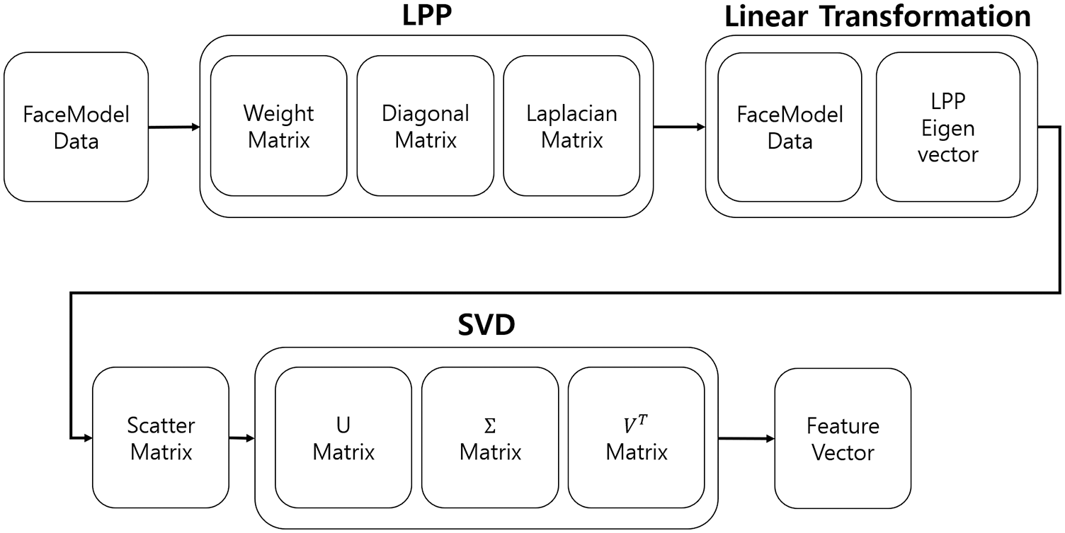
Figure 1: System process

4.1 Combined PCA-LPP

LPP is an effective method for finding feature vectors when data are nonlinear manifolds. However, when a feature vector is constructed using only LPP, most feature vectors must be used for reconstruction because feature values are almost identical. As PCA considers only the overall characteristics of the data, the reconstruction of detailed parts may be insufficient. Therefore, we solved this problem by combining PCA and LPP. Additionally, traditional PCA-LPP combination methods [21,22] focus on obtaining a set of data through an appropriate data distribution, such as classification or clustering. In some cases, this is unsuitable for data reconstruction as it can severely damage the original data features and prevent the natural movement of the mesh during reconstruction. When reconstructing a face, the mesh should change naturally, and the features should be emphasized. In this case, the features must preserve local features, such as the connection relationship between vertices, to preserve the details of the face model. We preserved the local feature with LPP before using PCA. Hence, the LPP weight matrix is defined as an adjacency matrix composed of connections between the vertices of the face mesh. Therefore, weights between connected vertices are 1. Subsequently, the LPP problem is solved using the input as the transposed data matrix XT, and the matrix L of the extracted feature vectors is extracted.

Data matrix X is transposed as the common connection relation of the data and used as the weight matrix. After solving the LPP problem, data matrix T is constructed using T=XLT. The PCA problem is solved based on the constructed data matrix T. The extracted vectors and values were used as the feature vectors of the 3DMM. This can be expressed as follows in pseudocode.

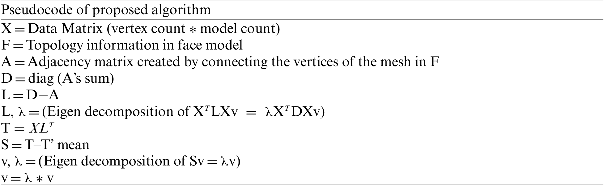
Pseudocode of proposed algorithm

4.2 3D Face Reconstruction

To test the performance of our proposed PCA-LPP method, we modified it to fit the open-source published Facewarehouse data [27]. A study [27] developed a program that can reconstruct a face from a single image or video, does not require prior learning through deep learning, and is characterized by directly estimating parameters using the error between facial landmarks and images.

Fig. 2 presents four steps, including reconstructing the face from a single image, detecting landmarks on the detected face, and tracking rigid and non-rigid features. 3D face reconstruction can be processed using the following four steps:

1)   Detecting face in a single image

Face detection is performed using a multitask cascaded convolutional neural network (MTCNN) [28]. The MTCNN method consists of three convolutional networks: P-Net, R-Net, and O-Net. As it uses three convolutional network structures, it can detect all small faces in the image and shows high accuracy. To use the MTCNN, all three convolutional networks must be trained. The Facenet-Pytorch library [29,30] is advantageous because it can use a trained MTCNN quickly and easily. The Facenet-Pytorch library was used in this study.

2)   Detecting face landmarks on the detected face

Dlib [31] was used for face landmark detection. We used 74 landmarks instead of the 68 landmarks in Facewarehouse. Because Facewarehouse is reconstructed using 74 landmarks from the RGBD raw data, a higher reconstruction rate can be expected with the same number of landmarks. In addition, the 74-landmark system further details the nose range than the 68. Facewarehouse has its own pose image files of 150 (people) × 20 pixels and uses them as input for learning. Facewarehouse’s landmarks have increased the number of landmarks on the nose and eyebrows compared with the existing landmarks.

3)   Rigid tracking

Face reconstruction consists of two processes: rigid and non-rigid tracking. Rigid tracking is the process of aligning a face in an image with the prepared template model. The template model is the average face model of the Facewarehouse database, and when aligning the model and face in the image, it is sorted based on the landmark of the face. The template model is rotated and translated until the L2 norm between the landmark of the image acquired using dlib and the landmark of the projected template model is minimized.

Loss=Wk∗Landmarkloss.

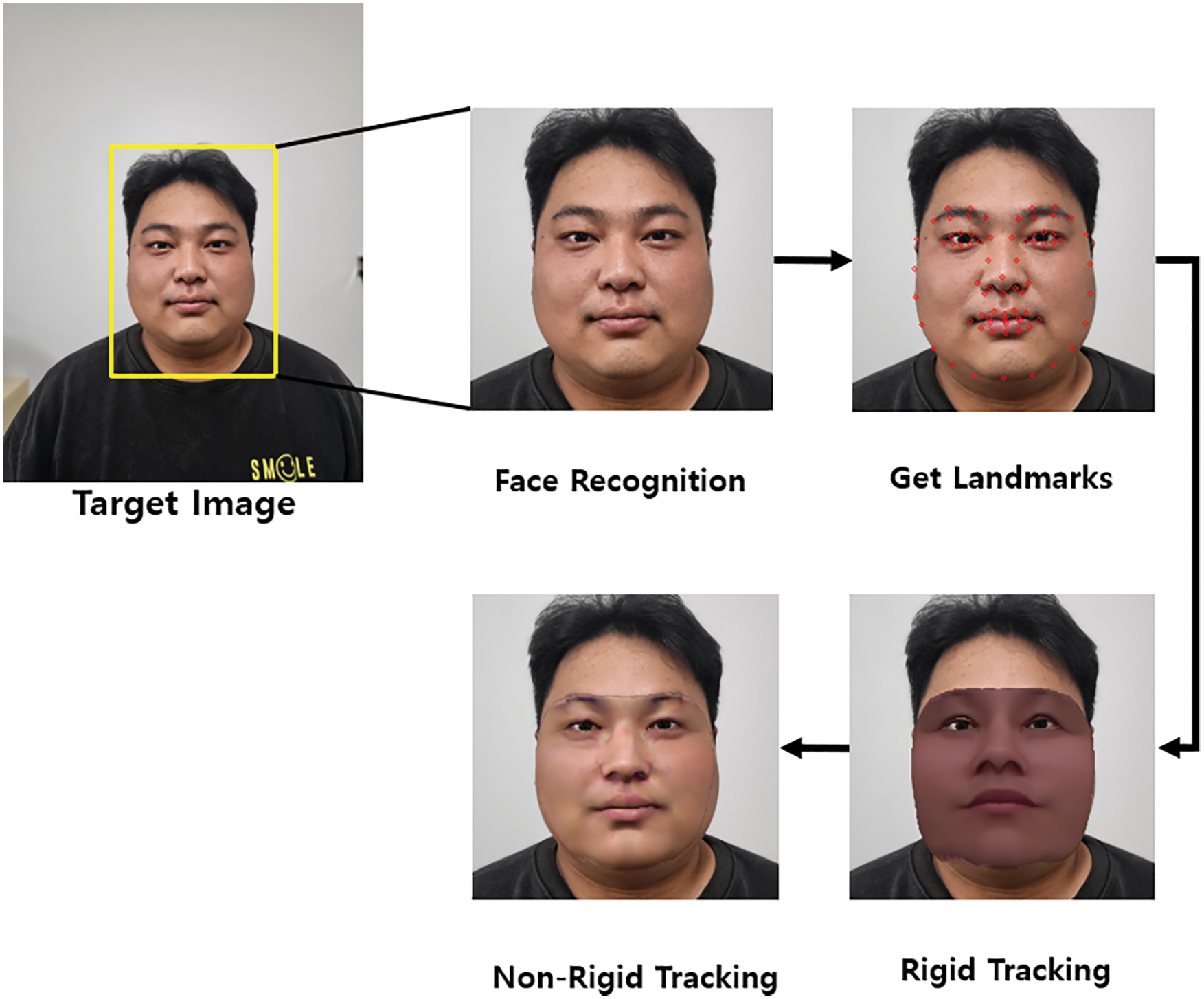
Figure 2: Face reconstruction process

Fig. 3 shows the results of the detection of 74 landmarks from an image using dlib. As shown in (a), landmarks can be effectively detected in the frontal image, and no problem occurs in detecting landmarks even if they are not frontal and have facial expressions, as shown in (b).

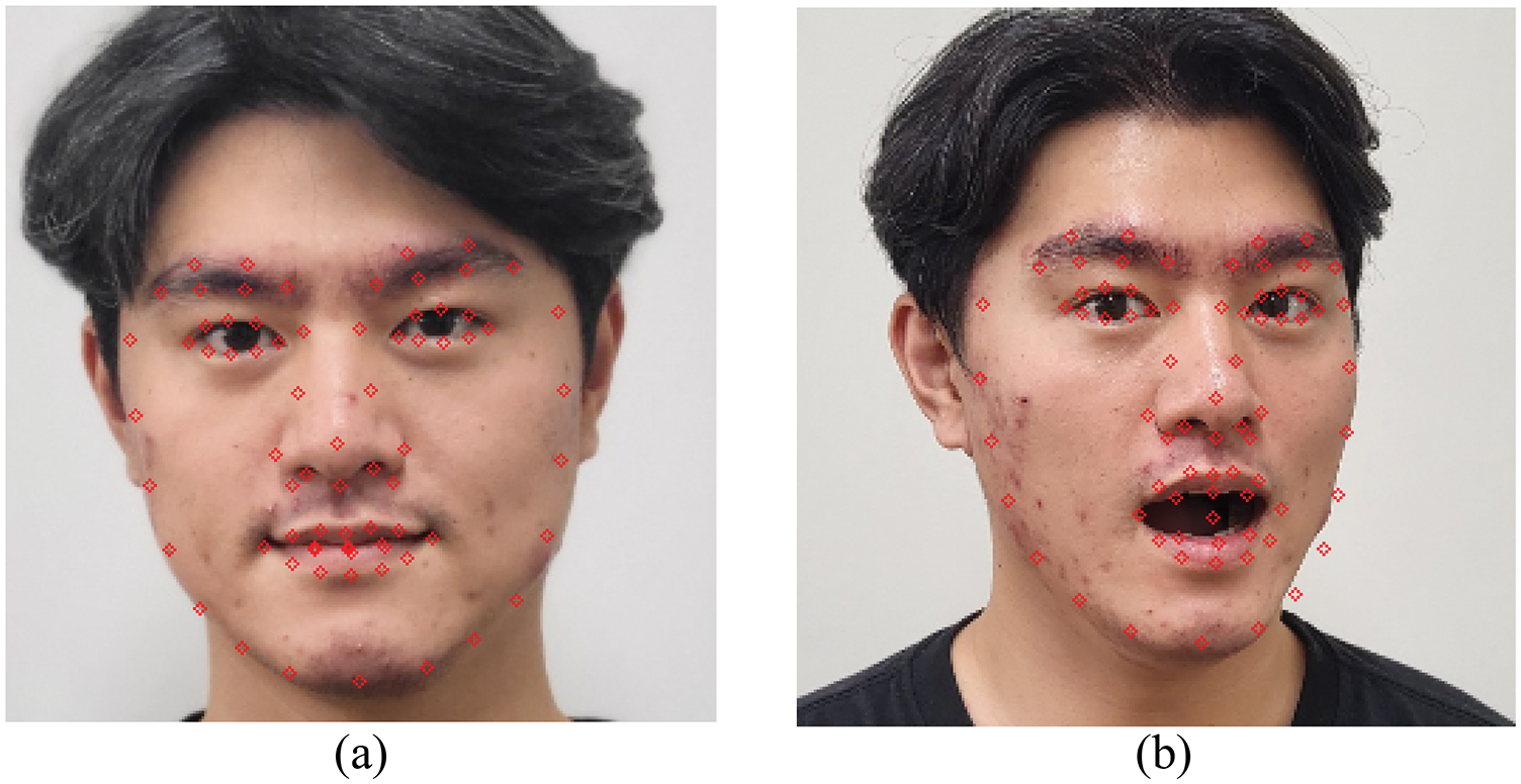
Figure 3: Dlib results. (a) Detects a landmark from an expressionless frontal image. (b) Landmark detected from the lateral image with the mouth open. Both images detect 74 landmarks

Rigid tracking uses landmark loss with the L2 norm as a process to match the original image’s size and orientation to the template model. Wk is the regularization weight of the landmark loss. The landmark loss is expressed in Eq. (2) as follows:

Landmarkloss=∑k=1nλk⋅(ykland−xklandM)2n,(2)

where n denotes the number of landmarks and M denotes the image size. ykland are the coordinates in the image where the 3D landmark vertices in the model are projected, and xkland are the 2D landmark coordinates detected in the original image. We assigned more weight to the landmarks corresponding to the eyes and nose for quick and accurate alignment and then proceeded with rigid tracking.

As shown in Fig. 4, the face model and face in the image were aligned through rigid tracking. Rigid tracking is optimized with landmark loss and can be effectively aligned in both frontal (a) and side (b) images. Even with the same expression as in (b), the template model without expression determines the angle and position that minimizes landmark loss; therefore, alignment is not a problem.

4)   Non-rigid tracking

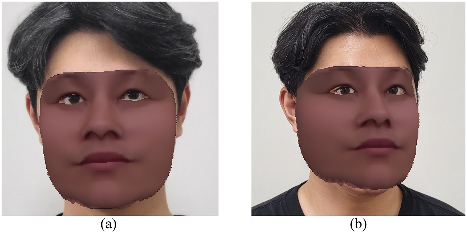
Figure 4: Rigid tracking results. (a) Frontal image, with the template model aligned in the front. (b) Looking to the side, with the template model aligned at the same angle as the face in the image

Non-rigid tracking optimizes the aligned template model equally to the face in the image. In this step, the identity, texture, and expression coefficients that determine the appearance of the model are estimated using the L2 loss as follows:

Loss=λ1∗Landmarkloss+λ2∗Photoloss+λ3∗∑idcoeffs2+λ4∗∑expcoeffs2+λ5∗∑texcoeffs2.

Here, λ1,λ2, …, λ5 are the regularization weights applied to each term. To prevent the parameter from becoming excessively large or a local minimum in the process of estimating each parameter, we included a regularization term that weights the error as follows:

Photoloss=∑k=1n∑l=1mWk⋅||yk,l−xk,l||2255.

where n and m denote the width and height of the image, respectively, yk,l denotes the RGB value of the image pixel rendered by the model, and xk,l denotes the RGB value of the original image pixel. Wk is a skin mask that checks whether the mesh is expressed as pixel coordinates, and only pixels with face meshes are included in the loss calculation.

Fig. 5 shows the results of non-rigid tracking, which are reconstructed by estimating each coefficient value. The two models (Fig. 5) were reconstructed to the same skin color as the photo by estimating the texture coefficient. Non-rigid tracking is a process of reconstructing a face model by optimizing the identity, expression, and texture coefficients by comparing images and models.

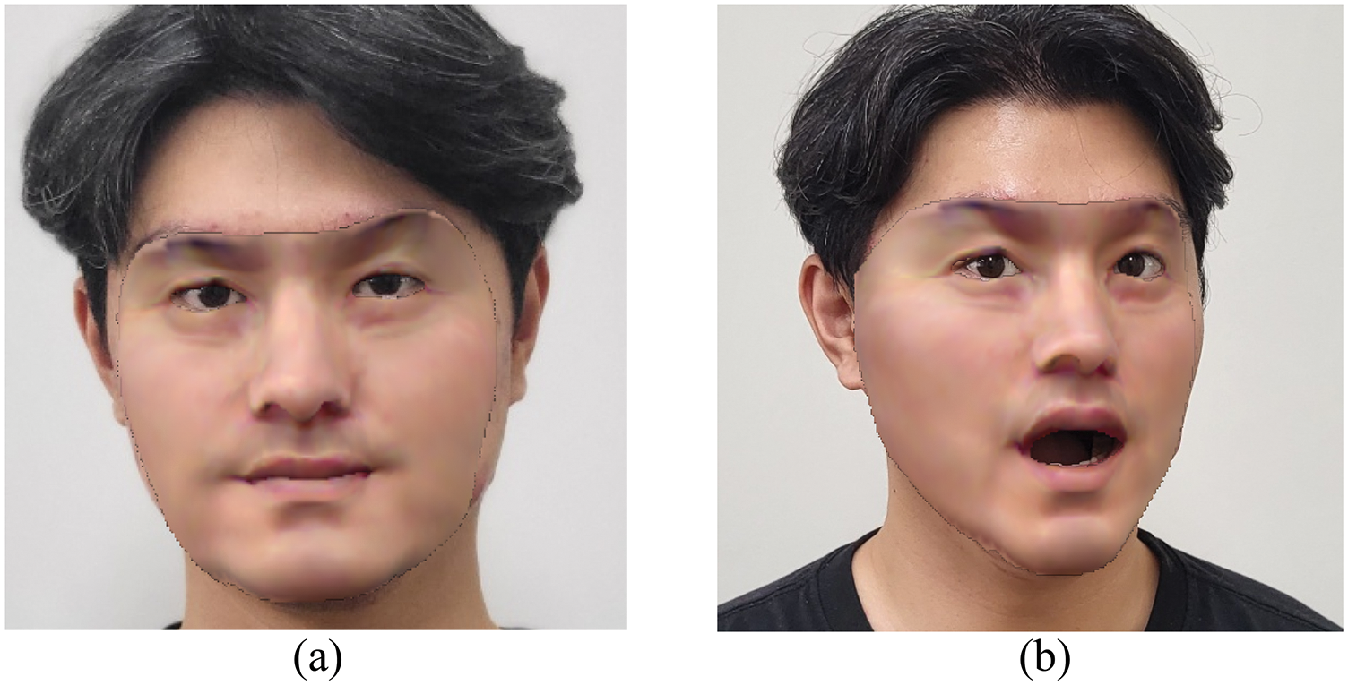
Figure 5: Non-rigid tracking results. (a) and (b) perform non-rigid tracking using the feature vector extracted using the proposed method

5  Experiment

5.1 Environment

This section introduces the experimental environment used to reconstruct a face from a single image. The operating system performed deep learning and experimentation using MS Windows 10. One Nvidia GeForce RTX 3080Ti GPU was used for deep learning, as well as Python 3.8. Pytorch3D [32] was used for rendering and deep learning training. Pytorch3D is a library for deep-learning-based 3D computer vision research released in 2020. The Adam optimizer was used for deep learning, and the learning rate was set to 1e−2. Image and landmark losses were weighted at 100 and 1.3, respectively. For regularization, the identity, expression, and texture regularization were set to 0.2e−1, 0.8e−3, and 1.2e−2, respectively. We experimented with face models and textures for learning based on face data from Facewarehouse. Facewarehouse contains information on facial models, images, and landmarks. Additionally, Facewarehouse is suitable for evaluating the reconstruction rate because it creates a face model based on a face image.

5.2 Evaluation

To evaluate the proposed method, face reconstruction was performed using an image provided by Facewarehouse, and the reconstructed model was evaluated by comparing it to the original face model provided by Facewarehouse. For comparisons between algorithms, the error of the reconstruction results using the proposed method and those using the PCA or LPP algorithms alone were compared with the original model. Landmark and photo losses acquired during tracking are the results to be compared with the image input for reconstruction; therefore, they are unsuitable for the evaluation and excluded from the evaluation process. We calculated the L2 norm between the vector and original model using the face image in Facewarehouse as input.

The evaluation method measures and compares the model loss, which is given by Eq. (3) as follows:

Modelloss=∑k=1n||yk−xk||2n,(3)

where n denotes the position of the vertices of the original model, yk denotes the position of the vertices of the original model (Model Num = k), and xk denotes the position of the vertices of the reconstructed model (Model Num = k). The model loss measured using Eq. (3) was normalized to 0–1. If the errors of the models are normalized, the weight of each error can be reflected equally.

5.3 Result

Table 1 lists the average errors for the reconstructed results obtained using the three methods. The face models were provided by Facewarehouse, and all models have the same vertices #5,282 and tris #10,308. The reconstruction results in Table 1 indicate that the proposed method has less errors than the PCA and LPP methods.

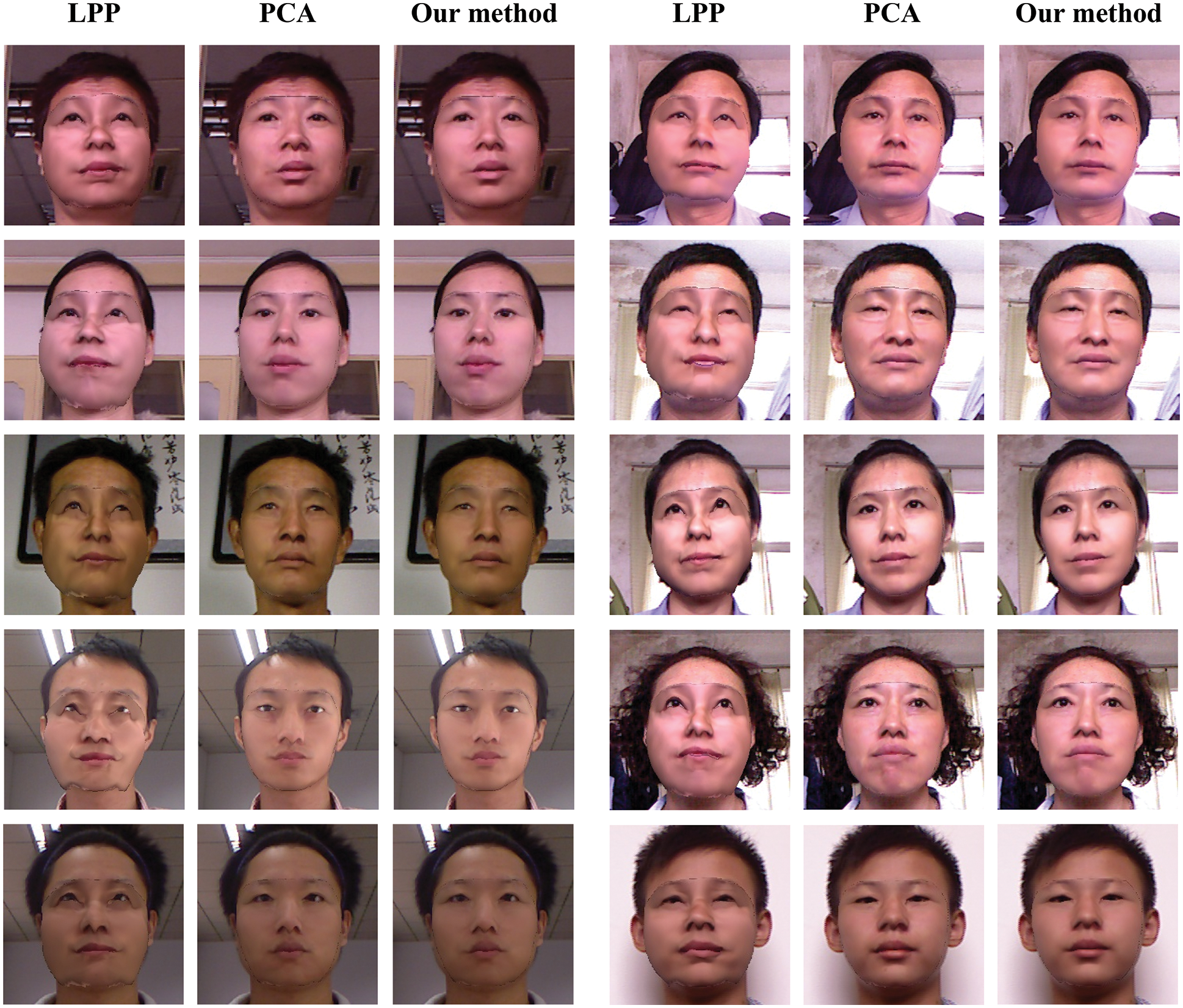
Fig. 6 shows the results of face reconstruction using images provided by Facewarehouse. The four face models used 150 feature vectors, and the reconstruction results with a 3D face model are shown. We compared the reconstructed face models using the PCA and LPP algorithms with the proposed method. Evidently, the LPP method did not effectively reconstruct the face, whereas the PCA and proposed method reconstructed the face effectively. In particular, when comparing the PCA and proposed method, the overall reconstruction was similar, but differences are noticeable in the detailed and complex parts, such as in the wrinkles of the eye and lip areas.

Figure 6: Face reconstruction with proposed method

5.4 Discussion

We compared the reconstructed face models using the PCA and LPP algorithms with the proposed method. The reconstruction results in Table 1 indicate that the proposed method has 10%–20% less errors than the PCA and LPP methods. In Fig. 6, the LPP method did not effectively reconstruct the face, whereas the PCA and proposed method reconstructed the face effectively. In particular, when comparing the PCA and proposed method, the overall reconstruction was similar, but differences were noticeable in the detailed and complex parts, such as in the wrinkles of the eye and lip areas.

However, because the proposed method includes both global and local feature, it is easier to get stuck in local minima problem than the PCA, which values global information. In addition, the reconstruction performance is notably reduced in cases where the face direction exceeds 30 degrees in a large pose or concealed part of the face. Thus, to obtain good results using the proposed method, using input image that face the front and avoiding the local minima problem, such as regularization, is important.

6  Conclusions

In this paper, we proposed a combined PCA-LPP algorithm that improves the existing feature vector extraction method to improve the 3D face reconstruction performance. Unlike the existing PCA-LPP method, the focus was on 3D face reconstruction, and the combined PCA-LPP algorithm was implemented using the 3D face mesh as an adjacency graph. The combined PCA-LPP algorithm exhibited a better reconstruction performance than the existing 3D face reconstruction methods implemented with feature vectors extracted from PCA and LPP. In particular, the performance improved by 10%–20% compared with the PCA algorithm, which is often used in the existing face reconstruction field. Therefore, the combined PCA-LPP algorithm yielded better results than the conventional method for 3D face reconstruction, as demonstrated by our results.

However, the proposed method was used only for 3D face reconstruction and is valid only for extracting the parameters of the feature vectors without training on the Facewarehouse dataset. In future work, we plan to compare the loss using feature vectors extracted from databases other than Facewarehouse. In this research, because the reconstruction rate of large pose face images was not excellent, we intend to search for a landmark method that is good for large poses and increases the face reconstruction rate by applying a neural network structure.

Acknowledgement: Thanks to Professor Kun Zhou for supporting Facewarehouse at Zhejiang University.

Funding Statement: This research was supported by the Basic Science Research Program through the National Research Foundation of Korea (NRF), funded by the Ministry of Education (2021R1I1A3058103).

Conflicts of Interest: The authors declare that they have no conflicts of interest to report regarding the present study.

References

1. N. Ersotelos and F. Dong, “Building highly realistic facial modeling and animation: A survey,” The Visual Computer, vol. 24, no. 1, pp. 13–30, 2008. [Google Scholar]
2. V. Blanz and V. Thomas, “A morphable model for the synthesis of 3D faces,” in Proc. Computer Graphics and Interactive Techniques, Los Angeles, CA, USA, pp. 187–194, 1999. [Google Scholar]
3. K. Genova, F. Cole, A. Maschinot, A. Sarna, D. Vlasic et al., “Unsupervised training for 3D morphable model regression,” in Proc. Computer Vision and Pattern Recognition, Salt Lake, UT, USA, pp. 8377–8386, 2018. [Google Scholar]
4. A. T. Tran, T. Hassner, I. Masi and G. Medioni, “Regressing robust and discriminative 3D morphable models with a very deep neural network,” in Proc. Computer Vision and Pattern Recognition, Honolulu, HI, USA, pp. 5163–5172, 2017. [Google Scholar]
5. Y. Deng, J. Yang, S. Xu, D. Chen, Y. Jia et al., “Accurate 3D face reconstruction with weakly-supervised learning: From single image to image set,” in Proc. Computer Vision and Pattern Recognition, Long Beach, CA, USA, pp. 1–11, 2019. [Google Scholar]
6. P. Dou, S. K. Shah and I. A. Kakadiaris, “End-to-end 3D face reconstruction with deep neural networks,” in Proc. Computer Vision and Pattern Recognition, Honolulu, HI, USA, pp. 5908–5917, 2017. [Google Scholar]
7. A. S. Jackson, A. Bulat, V. Argyriou and G. Tzimiropoulos, “Large pose 3D face reconstruction from a single image via direct volumetric CNN regression,” in Proc. Int. Conf. on Computer Vision, Venice, Italy, pp. 1031–1039, 2017. [Google Scholar]
8. Y. Feng, F. Wu, X. Shao, Y. Wang and X. Zhou, “Joint 3D face reconstruction and dense alignment with position map regression network,” in Proc. Computer Vision and Pattern Recognition, Munich, Germany, pp. 534–551, 2018. [Google Scholar]
9. Y. Chen, H. Wu, F. Shi, X. Tong and J. Chai, “Accurate and robust 3D facial capture using a single RGBD camera,” in Proc. IEEE Int. Conf. on Computer Vision, Sydney, Australia, pp. 3615–3622, 2013. [Google Scholar]
10. G. J. Hsu, Y. Liu, H. Peng and P. Wu, “REG-D-based face reconstruction and recognition,” IEEE Transactions on Information Forensics and Security, vol. 9, no. 12, 2014. [Google Scholar]
11. F. Adnan, J. Ahmad and K. Shaharyar, “Dense RGB-D Map-based human tracking and activity recognition using skin joints features and self-organizing map,” KSII Transactions on Internet and Information Systems, vol. 9, no. 5, pp. 1856–1869, 2015. [Google Scholar]
12. F. Adnan, J. Ahmad and K. Shaharyar, “Detecting complex 3D human motions with body model low-rank representation for real-time smart activity monitoring system,” KSII Transactions on Internet and Information Systems, vol. 12, no. 3, pp. 1189–1204, 2018. [Google Scholar]
13. J. Booth, A. Roussos, A. Ponniah, D. Dunaway and S. Zafeiriou, “Large scale 3D morphable models,” International Journal of Computer Vision, vol. 126, no. 2–4, pp. 233–254, 2018. [Google Scholar]
14. C. Cao, Y. Weng, S. Zhou, Y. Tong and K. Zhou, “Facewarehouse: A 3D facial expression database for visual computing,” Visualization and Computer Graphics, vol. 20, no. 3, pp. 413–425, 2013. [Google Scholar]
15. B. Egger, W. A. P. Smith, A. Tewari, S. Wuhrer, M. Zollhoefer et al., “3D morphable face models—past, present, and future,” Graphics, vol. 39, no. 5, pp. 1–38, 2020. [Google Scholar]
16. A. Maćkiewicz and W. Ratajczak, “Principal components analysis (PCA),” Computers & Geosciences, vol. 19, no. 3, pp. 303–342, 1993. [Google Scholar]
17. P. H. Truong, C. Park, M. Lee, S. Choi, S. Ji et al., “Rapid implementation of 3D facial reconstruction from a single image on an android mobile device,” KSII Transactions on Internet and Information Systems, vol. 8, no. 5, pp. 1690–1710, 2014. [Google Scholar]
18. A. Jourabloo and X. Liu, “Large-pose face alignment via CNN-based dense 3D model fitting,” in Proc. Computer Vision and Pattern Recognition, Las Vegas, NV, USA, pp. 4188–4196, 2016. [Google Scholar]
19. X. He and P. Niyogi, “Locality preserving projections,” in Proc. Neural Information Processing Systems, Cambridge, MA, USA, pp. 153–160, 2003. [Google Scholar]
20. A. Kim, C. Wang and S. Seo, “PCA-CIA ensemble-based feature extraction for Bio-key generation,” KSII Transactions on Internet and Information Systems, vol. 14, no. 7, pp. 2919–2937, 2020. [Google Scholar]
21. C. Chen, R. Bie and P. Guo, “Combining LPP with PCA for microarray data clustering,” in Proc. Congress on Evolutionary Computation, Hong Kong, China, pp. 2081–2086, 2008. [Google Scholar]
22. Z. Zhang, X. Zhu, J. Zhao and H. Xu, “Image retrieval based on PCA-LPP,” in Proc. Distributed Computing and Applications to Business, Engineering and Science, Wuxi, China, pp. 230–233, 2011. [Google Scholar]
23. L. Yin, X. Wei, Y. Sun, J. Wang and M. J. Rosato, “A 3D facial expression database for facial behavior research,” in Proc. Automatic Face and Gesture Recognition, Southampton, UK, pp. 211–216, 2006. [Google Scholar]
24. L. Tran and X. Liu, “Nonlinear 3D face morphable model,” in Proc. Computer Vision and Pattern Recognition, Salt Lake, UT, USA, pp. 7346–7355, 2018. [Google Scholar]
25. M. E. Wall, A. Rechtsteiner and L. M. Rocha, “Singular value decomposition and principal component analysis,” in A Practical Approach to Microarray Data Analysis, New York, NY, USA: Springer Science, pp. 91–109, 2003. [Google Scholar]
26. M. Belkin and P. Niyogi, “Laplacian eigenmaps and spectral techniques for embedding and clustering,” in Proc. Advances in Neural Information Processing Systems, Vancouver, BC, Canada, pp. 585–591, 2001. [Google Scholar]
27. AsCu, 3DMM-Fitting-Pytorch, 2021. [Online]. Available: https://github.com/ascust/3DMM-Fitting-Pytorch. [Google Scholar]
28. K. Zhang, Z. Zhang, Z. Li and Y. Qiao, “Joint face detection and alignment using multitask cascaded convolutional networks,” IEEE Signal Processing Letters, vol. 23, no. 10, pp. 1499–1503, 2016. [Google Scholar]
29. F. Schroff, D. Kalenichenko and J. Philbin, “FaceNet: A unified embedding for face recognition and clustering,” in Proc. Computer Vision and Pattern Recognition, Boston, MA, USA, pp. 815–823, 2015. [Google Scholar]
30. T. Esler, Facenet-pytorch, Melbourne, Australia, 2020. [Online]. Available: https://github.com/timesler/facenet-pytorch. [Google Scholar]
31. D. E. King, Dlib, Boston, MA, USA, 2022. [Online]. Available: https://github.com/davisking/dlib. [Google Scholar]
32. A. Paszke, S. Gross, F. Massa, A. Lerer, J. Bradbury et al., “PyTorch: An imperative style, high-performance deep learning library,” in Proc. Advances in Neural Information Processing Systems, Vancouver, BC, Canada, pp. 8026–8037, 2019. [Google Scholar]
Cite This Article
Copyright © 2023 The Author(s). Published by Tech Science Press.
This work is licensed under a Creative Commons Attribution 4.0 International License , which permits unrestricted use, distribution, and reproduction in any medium, provided the original work is properly cited.
Downloads
Citation Tools