Improving Brain Tumor Classification with Deep Learning Using Synthetic Data

1  Introduction

Non-invasive neuroimaging techniques can be used to diagnose and grade brain tumors, plan and guide the surgical process, as well as to monitor and evaluate response to treatment. In the analysis of brain tumors, classification of tumors and segmentation of tumor locations are performed. In classifying brain tumors, the variety of tumor types and their grade is provided using statistical similarities of images or by data obtained using feature analysis [1].

In recent years, artificial intelligence (AI) techniques such as machine learning (ML) methods and especially deep learning (DL) have frequently been used to analyze medical images [1,2]. ML is a research field of AI and enables the generalization of the data of a problem to make predictions by learning with approaches such as logistic regression and support vector machines. DL is one of the ML techniques based on artificial neural networks (ANN), inspired by the neuron and communication structure of the brain. DL has multiple processing layers, and it provides the learning of the representations of the data presented to the model by abstracting them at multiple levels in these layers [3]. By processing brain images, the two dimensional (2D) or three dimensional (3D) convolutional neural network (CNN) model, which is the first DL model [4], has achieved promising results in classifying diseases such as Alzheimer’s, schizophrenia, and stroke and in determining brain activity [2]. The main difference between CNN architecture and other ML techniques is that it does not require feature analysis. On the other hand, since CNN can have millions of trainable parameters, it needs large training data to reach adequate representative abstraction of the input data for a specific problem and a graphics processing unit (GPU) for computing requirements. For this reason, in the medical data analysis, the lack of a data set containing a sufficient number of samples with all the conditions of the problem makes it difficult to use DL. In this case, the overfitting problem occurs as a result of training with an insufficient dataset [2,5,6].

Data augmentation is a technique that helps improve the representative abstraction ability of the DL model and provides regularization of the network indirectly [6]. It plays an important role in improving accuracy, especially in medical studies, where the amount of data is limited and obtaining new samples is costly and time-consuming [6]. Data augmentation techniques preferred in data sets used to classify or segment brain tumors in the literature can be examined in two groups synthetic data generation or conversion from original data. When reproducing data from the original data, affine transformation, elastic transformation, or pixel-level transformations are performed [5]. With affine transformation techniques, images are reproduced by rotating, zooming, cropping, flipping, and translating. In data augmentation with the elastic transformation method, the shape of the training samples is changed. However, this process can cause a lot of noise and damage in images with a brain tumor. Also, excessive distortion and occurrence of the tumor in unsuitable places can create unreal synthetic images. While reproducing data from medical images with pixel-level transformations, it is desired to create the effect of obtaining data from different devices with different gradients or saturation. For this, it is ensured that medical images are reproduced by adding random or zero average Gaussian noise on the pixel/voxel intensities of the images, applying gamma correction, sharpening, blurring, shifting, or scaling pixels/voxels [5].

In recent years, many synthetic data generation techniques have been proposed to reproduce data on medical images. Conventional data augmentation techniques such as scaling, rotation, and flipping used to augment images do not consider the size, shape, position, or appearance of the anomaly in the image. Also, they do not take into account the differences or distributions available in imaging protocols such as magnetic resonance imaging (MRI), computed tomography (CT), positron emission tomography (PET), or functional MRI (fMRI). Generative adversarial network (GAN) architectures are widely used in medical image synthesis when the number of samples is insufficient [6]. The primary purpose of using the GAN is to discover the basic structures in training data and generate new ones that cannot be distinguished from real data [7]. The second purpose is to use the discriminator as a sensor to distinguish normal and abnormal structures in medical images [6]. Zhu et al. [8] proposed the cycle-consistent adversarial networks (CycleGAN) architecture for image-to-image transfer. This method basically captures the distinguishing features in one image and transfers them to another image without a set of labeled samples paired with each other. For this reason, CycleGAN architecture achieves successful results in image transfer and cross-modality image synthesis on medical images [9–12]. Especially for brain images, the CycleGAN architecture synthesizes enhanced images close to reference images [9–12]. In addition, data augmentation using CycleGAN and then the classification of lung opacities or Alzheimer’s diseases using CNN with augmented data improved the performance results [13,14].

This study aimed to produce T1-weighted (T1W) MR brain images including three different brain tumors (glioma, meningioma, and pituitary) in the figshare brain dataset using DL due to limited data in hand and then classifying them to facilitate diagnosis and treatment in the clinic. First, axial, coronal, and sagittal slices of each tumor type in the data set were separated. Second, using these separated images, CycleGAN architecture generated new slices for each tumor. For example, two different images were selected randomly for the glioma tumor’s axial slice, and the distinctive features in the first image were determined and transferred to the second image. Thus, it was not allowed to transfer between different tumor types and different slices in order to protect the tumor characteristics and brain structure. Finally, the original training set was combined with the synthetic images, and these images were used as input to the CNN to classify brain tumor types. CNN architecture has been created according to the dense convolutional network (DenseNet121) architecture. The labeled outputs and CNN precision results were evaluated with precision, recall, F1 score, accuracy, specificity, Pearson correlation coefficient, and area under curve (AUC) measurements.

2  Review of the Existing Methods in Brain Tumor Classification

In this study, brain tumor classification was performed with DL by generating synthetic data. For this reason, ML approaches performed on the figshare brain dataset followed by a literature review on DL-based studies, and CycleGAN-based data augmentation studies for medical images are given in this section.

The most widely used technique for detecting abnormalities in the brain is the MRI technique. Early detection of brain tumors in MR images is essential for treatment planning. The main difficulty encountered in multiclass brain tumor classification is finding information to distinguish the tumor from normal brain tissue in images [15–17]. The brain tumor classification methods in the literature can be performed in two steps: feature extraction and classification. In feature extraction, the whole brain is examined, or the brain is divided into a region of interest (ROI) and a region of non-interest (RONI). In the classification, the obtained features are used in training and testing an ML model. Decision tree, k-nearest neighbor (k-NN), Bayes, support vector machine (SVM), linear discriminant analysis (LDA), and multi-layer perceptron (MLP) are widely used classifiers in supervised learning.

Brain tumors have patient-specific shapes and gray-level intensities, and tumors with different pathologies may resemble each other in the image. These conditions make it challenging to distinguish tumors from brain structures and each other. For this reason, it is difficult to identify the correct features to be used in brain tumor classification. In the literature, DL techniques, which obtain features in the internal layers and do not require complex pre-processing, have achieved successful results on open datasets such as the brain tumor segmentation (BraTS), Internet brain segmentation repository (IBSR), cancer imaging archive (TCIA), simulated brain database (BrainWeb), Alzheimer's disease neuroimaging initiative (ADNI), autism brain imaging data exchange (ABIDE), Ischemic Stroke Lesion Segmentation (ISLES), and figshare brain datasets for the classification and segmentation of brain images [1,18,19]. This study focuses on the classification of meningioma, pituitary tumor, and glioma brain tumors in MR images of the figshare brain dataset [18,19].

Cheng et al. [19] proposed a method for classifying brain tumors that include data augmentation, feature extraction, and classification steps. They augmented the data by applying morphological erosion and segmented them sub-ROIs by the fine ring-form method. They used intensity histogram, gray level co-occurrence matrix (GLCM), and bag-of-words methods for feature extraction. Bag-of-words and data augmentation operations increased the accuracy of the SVM classifier from 83.54% to 88.19%. After segmentation using fine ring form, the accuracy of the study was increased to 91.28%. Ismael et al. [20] classified brain tumors using statistical features and ANN. In the study, 2D Gabor filtering and discrete wavelet transform (DWT) were first applied to the manually segmented brain tumor regions. Then, the statistical features obtained from the coefficients of DWT were classified with ANN. The mean accuracy of the ANN model was 91.9%. In the other study [21], tumors were classified by SVM, which used the features obtained from the dense speeded up robust features (DSURF) and histogram of oriented gradients (HOG) methods, and the model’s accuracy value was obtained as 90.27%. Accordingly, complex feature analysis in these studies was performed on the figshare brain dataset [20,21]. According to the literature, it is unclear which features are effective or should be used together in the classification and segmentation of brain tumors [15–17]. For this reason, many studies in the literature provide tumor classification with DL models that perform feature analysis within their internal architecture.

Abiwinanda et al. [22] classified brain tumors in MR images using five CNNs. They have optimized their CNN architectures by using the different numbers of convolution layers and fully connected layers (FCLs). The selected CNN architecture (2 convolution layers with 64 filters, rectified linear unit-ReLU activation, and max-pooling layers) achieved a training accuracy of 98.41% and a test accuracy of 84.19%. However, test accuracy is lower than training accuracy indicating an overfitting problem. Widhiarso et al. [23] defined the GLCMs of tumor images and used them as the input of the CNN. The accuracy of the study was 80%. Alqudah et al. [24] generated 3 datasets containing the whole brain, cropped tumor images, and segmented tumor images for the brain tumor classification. The accuracy values of the CNN model for these 3 datasets with 128x128 image resolution are 98.77%, 97.39%, and 97.50%, respectively. Ayadi et al. [25] analyzed different brain tumor data using CNN. CNN model classified meningioma, glioma, and pituitary tumors with 95.23%, 95.43%, and 98.43% accuracy, respectively. Afshar et al. [26] classified brain tumors into three classes by focusing on the tumor’s boundaries with a capsule neural network (CapsNet). The accuracy of the CapsNet model was only 90.89%.

In the literature, there are studies using both data augmentation and transfer learning instead of optimizing the DL architecture. Bhanothu et al. [27] segmented tumor regions and classified the tumor types in images divided into ROIs with the faster region-based CNN (Faster R-CNN) model. VGG-16 architecture was used for the main structure in Faster R-CNN. The mean precision value of the study was found to be 77.60%. Rehman et al. [28] classified tumors by freezing and fine-tuning the three different CNN models (deep CNN-AlexNet, GoogLeNet, and Visual Geometry Group neural network-VGGNet). In addition, data augmentation (rotation and flipping) was used after contrast enhancement. Ghosal et al. [29] classified the segmented tumor images by CNN architecture instead of whole-brain images. CNN architecture has been transferred from the residual neural network (ResNet101). Squeeze and excitation blocks have been added to this architecture. In the study, the CNN was trained using both the original dataset and augmented dataset by flip, rotation, elastic transform, and shear methods. Data augmentation has increased the accuracy result from 89.93% to 93.83%. Badza et al. [30] trained the CNN architecture by 10-fold cross-validation with augmented data using rotation and flipping. The CNN model achieved an accuracy value of 96.56%. Sultan et al. [31] trained the CNN architecture with 16 layers using augmented data (flipping, mirroring, adding noise, and rotation), and the proposed model classified brain tumors with an accuracy of 96.13%. According to these studies, affine transformation and pixel-level transformation-based data augmentation have increased the accuracy of DL models [27–31].

In the literature, there are ML studies in which implemented using the features obtained from the layers of the DL architecture. Deepak et al. [32] transferred the layers and weights from GoogLeNet to CNN for brain tumor classification. In the study, the features taken from the last pooling layer of the CNN were used in SVM and k-NN methods. The accuracy results of CNN, SVM, and k-NN models were 92.3%, 97.8%, and 98.0%, respectively. Pashaei et al. [33] firstly obtained the features from the FCL of the CNN model, and then they classified the brain tumors by training kernel extreme learning machines (KELM) using these features. In the study, the CNN-based KELM method was compared with MLP, stacking, Extreme Gradient Boosting (XGBoost), SVM, and radial basis classifiers. The accuracy values of the other ML classifiers are 88.80%, 86.91%, 87.33%, 87.51%, and 86.84% respectively, and the accuracy value of the proposed method was found to be 93.68%. Gurkahraman et al. [34] classified brain tumors in three stages. First, they transferred the weights of the DenseNet121 network to the CNN architecture, and then the CNN was trained using the augmented images by applying affine transformation and pixel-level transformation. They used the features taken from the FCL of the trained CNN model as input to SVM, k-NN, and Bayes classifiers. The accuracy values obtained by CNN and CNN-based SVM, k-NN, and Bayes classifiers are 0.9860, 0.9979, 0.9907, and 0.8933, respectively. According to the results, the features obtained from the FCL of the CNN architecture increased the accuracy of ML classifiers [32–34].

Pathologies in medical images are evaluated using different image modalities (MR, CT, PET, fMRI, etc.). For this reason, unsupervised GAN models that perform cross-modality synthesis in data augmentation have been proposed in the literature. CycleGAN provides unsupervised image-to-image transfer using a combination of adversarial loss and cycle-consistency loss without paired samples [8,9]. CycleGAN has been used to synthesize cross-modality images and remove artifacts from medical images [9–12]. Mabu et al. [13] proposed a CycleGAN+CNN model to classify the opacity of lung diseases. CycleGAN with a domain transform approach was used to augment chest CT images collected from two hospitals. In another study [14], MRI images were augmented with CycleGAN to distinguish Alzheimer's disease from the healthy, and the resulting data were classified using the ResNet50 model. Augmented data has improved the classification performances of CNNs [13,14].

Compared to traditional data augmentation techniques that apply different transformations to existing data, CycleGAN has a more remarkable ability to generate new data that ML has not seen before because the augmented images by traditional techniques are only geometric and pixel-based replicas of existing images. In terms of GAN type selection, CycleGAN produces more acceptable synthetic images compared to other widely used GAN models based on similarity metric evaluations [35]. In addition, CycleGAN is superior to other GAN models because it does not require paired datasets, does not have the risk of disappearing of gradient, and is more successful in the case of a small amount of data [35,36]. For this reason, this study proposes a CycleGAN data augmentation+CNN classification model with residual blocks for classifying brain tumors. The contributions of this study to the literature are as follows:

– Producing synthetic T1W brain MR images for the first time in the figshare brain dataset including three tumor types (glioma, meningioma, and pituitary) using CycleGAN,

– Classification of brain tumors with images obtained after data augmentation for figshare brain dataset,

– Determining the effect of synthetic data in the CNN model for brain tumor classification.

3  Material and Methods for Brain Tumor Classification

In this study, a framework shown in Fig. 1 is proposed to generate synthetic 2D T1W MR images of three different brain tumors in the figshare brain dataset for the first time using CycleGAN architecture, and then classify them with the CNN model. In the first step, the images were split into training and testing datasets as 80% and 20%. 3 different tumors in the training dataset and their axial, sagittal, and coronal slices were augmented separately with 9 CycleGAN models. Images obtained after data augmentation were combined with original images. In the second stage, a CNN model was developed to classify brain tumor images. The DenseNet121 architecture proposed for the ImageNet dataset has been used to construct CNN architecture. In the last stage, the CNN was trained using the real and synthetic images and tested using real images in the testing dataset. The precision results were compared with the labeled outputs with precision, recall, F1 score, accuracy, specificity, Pearson correlation coefficient, and AUC methods.

Figure 1: Flow diagram of the proposed DL model for brain tumor classification

3.1 Data Processing

In this study, the figshare brain dataset [18,19] and augmented images were used for brain tumors classification. In Table 1, the numbers of 2D T1W MR images (axial, coronal, and sagittal) of 233 patients in the figshare dataset are given. The numbers of augmented images and the combination of original and augmented data with respect to tumor types are also seen in Table 1. The DenseNet121 architecture proposed for the ImageNet dataset has been used to construct CNN architecture. For this reason, the input images have been resized to 128 × 128. When resizing, the loss of structural information in images should be kept to a minimum. In order to achieve this, first, the edges were detected in the images. Then, depending on the minimum and maximum row and column values of the edges, the dimension to which the longest ROI belongs was reduced to 128. Accordingly, the other ROI dimension was adjusted while maintaining the same ratio. The mean value of the background was also assigned to the RONI. Gray level values of the images presented as input to CNN were normalized between 0–1.

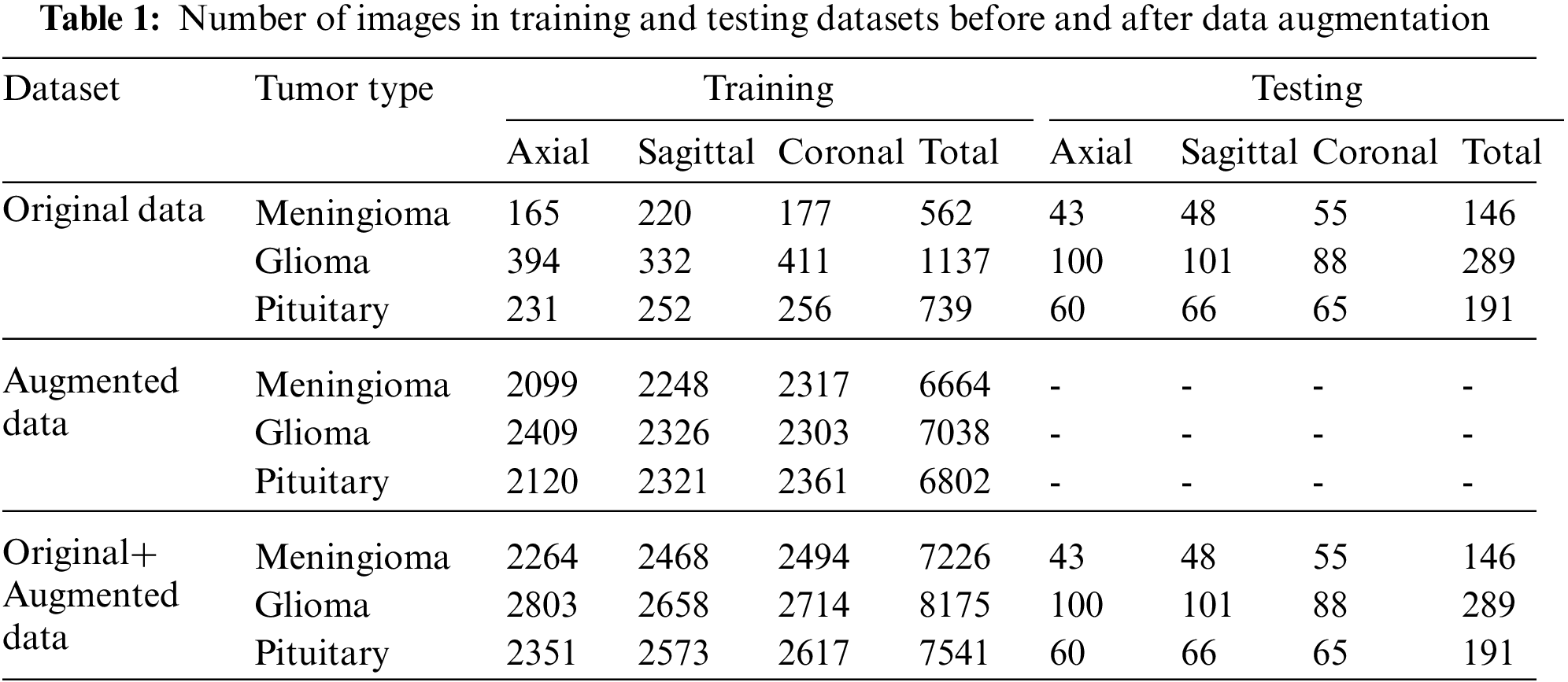
Before data augmentation, the dataset was split into 80% training and 20% test data. Then, the training data was augmented with CycleGAN for each tumor type and MR slice type (axial, coronal, and sagittal). The number of axial, sagittal, and coronal slices belonging to three tumors before and after data augmentation are shown in Table 1.

3.2 Data Augmentation with CycleGAN

In this study, the CycleGAN architecture used to produce synthetic brain tumor images is an unsupervised GAN architecture. In the CycleGAN model shown in Fig. 2, training is carried out by transferring from the source domain A to the target domain B, where domains A and B are the image pair consisting of unmatching 2D or 3D images. CycleGAN consists of four main components, two generators (GAB:A→B,GBA:B→A) and two discriminators (D1,D2). The first generating network (GAB) takes an input image x ϵ A from the source domain and produces the synthetic output y^=G1(x). The D1 network receives the synthetic output of GAB (y^) and a randomly selected image from target domain B (yϵB) as input. The D1 network behaves like a binary classifier to distinguish between the transferred image and the real image on the target domain. The GAB network also improves the translated image it produces to deceive the D1 network. The adversarial loss function between the two networks (Ladv(GAB;D1)) is given in Eq. (1) [37–39].

minGABmaxD1Ladv(GAB,D1)=Ey[log⁡(D1(y))]+Ex[log⁡(1−D1(GAB(x)))](1)

Figure 2: Architecture of CycleGAN

In CycleGAN, Ladv(GBA;D2) is the loss function of the second generator and discriminator networks. Networks GBA and D2 take y image as input and transfer x^ image as output. Training the CycleGAN architecture using only adversarial losses values can cause mode collapse due to the mapping of different views to a single view. For this reason, in the CycleGAN architecture, constraints that will force GAB and GBA to work cyclically together are added to the loss function. Accordingly, the two generators invert each other x^^=GBA(GAB(x))≈x and y^^=GAB(GBA(y))≈y. The inversion is done using pixel-wise cycle-consistency loss given in Eq. (2) in both generators [37–39].

Lcyc(GAB,GBA)=Ex[‖x−GBA(GAB(x))‖1]+Ey[‖y−GAB(GBA(y))‖1](2)

In this study, 9 separate CycleGAN were trained for each brain tumor class and each axial, coronal, and sagittal slices in order to generate data with preserved brain structural properties. The source input and the target input of each CycleGAN were selected randomly from the same MR slice of each tumor type. The CycleGAN was trained to obtain the feature maps of the source and target images (X, Y) and generated new images based on these feature maps. In CycleGAN, a translated Y image is obtained from a real X image presented to the GAB network. The translated Y image and the real Y image are distinguished by the D1 network whether they are real or fake. The reconstructed X image is obtained with the GBA network where the translated Y image is input. Similarly, a translated X image is obtained from the real Y image presented to the GBA network. The D2 network distinguishes the translated X and the real X image as real or fake. A reconstructed Y image is also obtained with the GAB network where the translated X image is input. In this study, reconstructed X and Y synthetic images were used in the training of CNN.

It was ensured that a source and target image pair was not replicated in the training dataset so that the simulated data was not a copy of the already generated one. In addition, the threshold value was used in CycleGAN training to eliminate unrealistic results produced due to instants of system instability. This value was determined as 5% of the total number of pixels in the ROI other than the background in the target image. After the generation of synthetic images, the augmented dataset was combined with real images and used in the training of CNN architecture. The pseudo-code of the image generation algorithm is given in below.

3.3 Transfer Learning-Based CNN Model

The deepening of CNN architectures leads to forgetting previously learned information in the network. Feature maps of different sizes are used in the DenseNet network to solve the forgetting problem. The difference between ResNet and DenseNet is that ResNet uses the summation of all previous feature maps, whereas DenseNet concatenates them in each layer, as shown in Fig. 1 [40,41]. It has l inputs in a layer l in the DenseNet network with features from previous convolution layers. If there is an x0 image at the network entrance, the information is processed forward in each layer. In the DenseNet network, a nonlinear transformation Hl(⋅) is performed for each sublayer with an index of l. Hl(⋅) transformation includes batch normalization (BN), ReLU, pooling, and convolution [40,41].

In conventional CNN, the output xl generated by layer l is the input of the next layer l+1. This transition of information between layers is expressed by the nonlinear composite function xl=Hl(xl−1). In the ResNet network, an identity function is added to the nonlinear component by adding a skip-connection which bypasses the nonlinear transformation, and the formula is given in Eq. (3) [40,41].

xl=Hl(xl−1)+xl−1(3)

The identity function used in ResNet allows the gradient to be transferred between layers. However, using the identity function and adding the output of Hl in the network delays the information flow. In the DenseNet network, each layer is directly connected to other sub-layers to solve the information flow problem in ResNet. In the DenseNet network, layer l takes the feature maps of previous layers (x0,…,xl−1) as input (Eq. (4)) [40,41].

xl=Hl([x0,x1,…,xl−1])(4)

Here, the Hl(⋅) function combines the inputs into a single tensor. BN, ReLU, and convolution operations are performed in the Hl(⋅) function. In DenseNet, the size of feature maps is reduced by down-sampling in pooling layers. The network is divided into dense blocks to facilitate the down-sampling process, and between these blocks, a transient layer is used, which includes BN, 1 × 1 convolution, and 2 × 2 pooling layers. There are 4 dense blocks in the DenseNet121 network shown in Fig. 1 [40,41]. In this study, the DenseNet121 network is used to prevent forgetting problems in the deep network and delay of information flow between layers. All the dense blocks used in our study had similar structures given in [40,41].

3.4 Experimental Setup

The proposed CycleGAN and CNN architectures were developed using Keras and Tensorflow libraries in the python programming language. The experiments were carried out on aPC with a 12 GB NVIDIA TITAN XP graphics card and i7 CPU. The Adam method was used for the optimization of the trainable parameters of the CycleGAN architectures. Learning rate and exponential decay rate values were set as 0.0002 and 0.5, respectively. Each image pair was used once to prevent the generation of similar images. Unrealistic images generated due to instants of system instability during CycleGAN training were eliminated using the threshold value. Two CNN models were constructed using DenseNet121 architecture. Using the 10-fold cross-validation technique, one of the architectures was trained with real images, and the other was trained with the combination of real and synthetic images. The numbers of neurons in two FCLs of DenseNet121 were 1024 and 512, and the dropout ratios of 0.3 and 0.2 respectively. BN was used after each FCL. The number of epochs was set to 100 and the batch size to 32. SGD method was used to update the weight and bias values in the CNN models. Momentum, learning rate, and decay values were selected as 0.9, 0.001, and 0.00001, respectively. Dropout and L2 regularization (Ridge Regression) were used to prevent the overfitting problem. Before data augmentation, 20% of the original data in Dataset-I was split for testing and 80% for training. Training data has been added to both the generation of synthetic images in CycleGAN and the training data of CNN. The real image dataset and the dataset that consists of real and synthetic images were split 90% as training and 10% as validation. In the study, three training experiments were done to designate the deep CNN network to be used in brain tumor classification. All experiments were repeated 10 times using cross-validation, and models were tested using the same test data. In the first experiment, the network was trained using the original training data, Dataset-I. In the second experiment, training was performed with only augmented training data using Dataset-II. In the third experiment, deep CNN was trained using Dataset-III containing augmented + original training data, and then tested with test data.

3.5 Evaluation Metrics

In this study, the performance results of the CNN model used in the classification of brain tumors were calculated by accuracy (Acc), specificity (S), AUC, precision (P), recall (R), and F1-score values. The equations of these metrics are given in Eqs. (5) and (6).

Acc=TP+TNTP+TN+FP+FN ,S=TNTN+FP(5)

P=TPTP+FP ,R=TPTF+FN,F1=2.Precision.RecallPrecision+Recall(6)

where TP, TN, FP, and FN are true-positive, true-negative, false-positive, and false-negative values, respectively.

4  Results and Discussion

In this section, the results obtained with the original and synthetic datasets are presented. In addition, the results were compared with the studies applying DL to the figshare dataset in the literature.

4.1 Experimental Results

In the study, 9 separate CycleGAN architectures were trained using axial, sagittal, and coronal slices of 3 brain tumor types, and synthetic images were generated. In Fig. 3, examples of source and target image pairs and reconstructed and translated images synthesized by CycleGAN are shown. In Fig. 4, the reconstructed images in different epochs and their difference images from source and target images are given. There are relatively large values in the difference images of the early epochs. The difference between the simulated images and target images in the later epochs has decreased, and the structural similarity has increased.

Figure 3: Real and synthetic image samples according to tumor classes and MR slices, (a) Glioma-axial, (b) Meningioma-sagittal, (c) Pituitary tumor-coronal

Figure 4: Real and synthetic images obtained in various epochs and their difference images (a) epoch 20, (b) epoch 50, (c) epoch 100, (d) epoch 150, (e) epoch 200

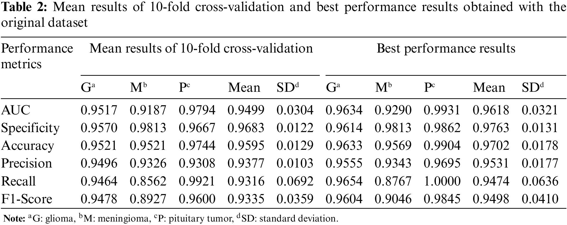
For the first experiment, Table 2 shows the mean and best performance results of CNN trained with 10-fold cross-validation using the original dataset. According to the mean and best results, the Pituitary tumor type has the highest accuracy value.

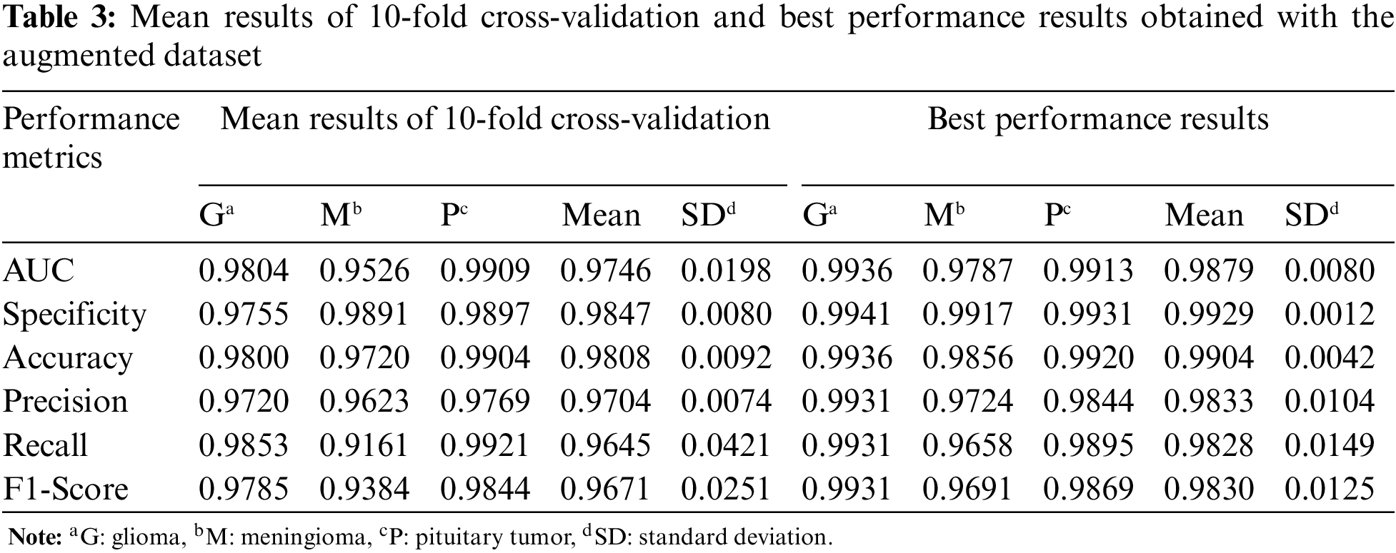
In Table 3, the mean and best performance results of CNN trained with 10-fold cross-validation using the augmented dataset, which includes the synthetic images, are given for the second experiment. Comparing the results in Tables 2 and 3, it is seen that the performance values of the augmented data are higher than the original data.

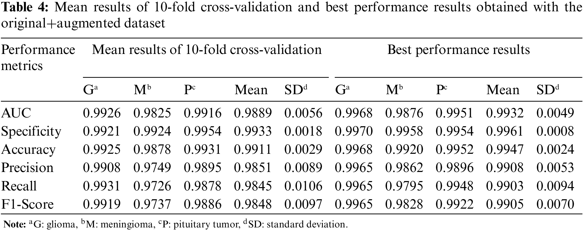
For the third experiment, the mean and best performance results of CNN trained with 10-fold cross-validation using the original+augmented dataset, which includes the real and synthetic images, are given in Table 4. Compared to the results obtained in the first two datasets, the performance results of the Glioma and Meningioma tumor types, which were relatively low, improved with the original+augmented dataset.

The confusion matrices of the CNN with best performances, which were trained with original, augmented, and original+augmented images and tested on the same test set, are given in Fig. 5. While there is a high confusion between glioma and meningioma tumors in the CNN model trained with original data, it is very low for the original+augmented data. In conclusion, CycleGAN has improved the brain tumor classification performance of the DL model.

Figure 5: Confusion matrices of CNN, (a) original dataset, (b) augmented dataset, (c) original +augmented dataset

4.2 Literature Comparison

In this study, we proposed a tumor classification model consisting of DenseNet121-based CNN and data augmentation with CycleGAN on the figshare brain dataset. In Table 5, the comparison of the results between our model and other proposed DL methods for the same dataset in the literature is given. More details about these studies are given in the literature review in Section 2. Examining ML studies on the figshare brain dataset, the accuracy values of ANN and SVM classifiers developed after different feature analyzes are between 0.9027 and 0.9190 [20,21]. Feature analysis and data augmentation increased the accuracy of the SVM classifier to 0.9110 [19]. In the literature, the accuracy values of ML classifiers using the features taken from the CNN layers as input were obtained between 0.8684 and 0.9979 [32–34]. In this study, deep CNN was used to classify brain tumors with high accuracy, without the need for feature analysis or dimension reduction.

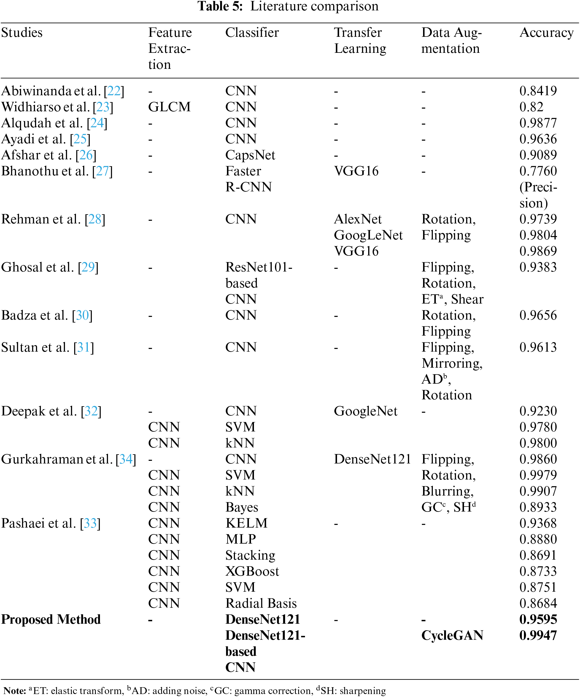
According to DL studies in the literature, the accuracy values of the CNNs that do not use data augmentation and transfer learning are between 0.82 and 0.9877 [22–25]. Accordingly, as the number of layers used in DL architectures increased, the accuracy value obtained for the figshare data set also increased [24,25]. The accuracy of the CNN architecture modeled by transfer learning using the GoogLeNet network was only 0.9230 [32]. In studies [30,31] using pixel-level data augmentation methods such as flipping, mirroring, adding noise, and rotation, the accuracy values of CNN architectures were calculated as 0.9656 and 0.9613, respectively. In studies using both data augmentation and transfer learning, the accuracy values of CNN architectures were obtained close to each other at 0.9860 and 0.9869 [28,34]. However, in [28], different CNN architectures using transfer learning were trained with data augmentation by rotation and flipping. The highest accuracy value was obtained with VGG16. In this study, it was not mentioned that the data augmentation was done after the test data was split. In [34], after data augmentation, all data were separated as training and test data. For this reason, the performance results of the CNN model were high since training and test data containing generated data from the original images. Therefore, the performance of ML techniques trained with features taken from CNN was also increased. In this study, the training and test data were separated before data augmentation, and the DL model was tested with data that were not used in the training process. Furthermore, in this study, DenseNet121 architecture was used for the design of the CNN model instead of architectural optimization, as DL models using transfer learning achieve high performance.

The pixel-level transformation (adding noise, blurring, and gamma correction), which is one of the conventional data augmentation methods, reduces the image quality [42]. Another traditional method is the elastic transformation which causes a lot of noise and damages the structure of the brain tumor. Rotating, flipping, or translating methods of the affine transformation increased data size without ensuring sample diversity in the dataset. Thus, it will not significantly improve the distinctive features of the classes it confuses. While GAN provides data diversity by producing realistic synthetic data, it does not cause the side effects of conventional methods on images. According to studies in the literature, realistic medical images similar to reference images are produced using CycleGAN [9–12]. The DL models using synthetic data achieve high performance in image enhancement, segmentation, perception, and classification problems [9–14]. For this reason, in this study, realistic brain images including tumors were produced using CycleGAN instead of using conventional data augmentation techniques such as affine transformation and pixel-level transformation. The accuracy values of the CNN model before and after the data augmentation were 0.9595 and 0.9947, respectively. In the most similar study [29], the images obtained by pixel-level data augmentation were classified with ResNet101-based CNN, and the accuracy of the study was found to be only 0.9383.

5  Conclusion

Brain tumors have patient-specific shapes and gray-level intensities. Also, tumors with different pathologies may resemble each other in the image. For this reason, it can be challenging to differentiate different types of tumors from one another or normal brain tissue. ML methods used for brain tumor classification in the literature require complex feature analyses, and it is unclear which of these analysis methods is more successful. DL techniques, which do not require complex pre-processing and feature analysis, are used in many areas of medicine and achieve promising results in brain tumor classification. This study proposes the DenseNet121-based CNN architecture for classifying glioma, meningioma, and pituitary tumors in the figshare brain dataset. The training dataset of the CNN was augmented using the simulated images with the CycleGAN architecture. Using CycleGAN, generated realistic brain images provide various data on tumor types, thus enabling a better classification of the classes it confuses. The use of CycleGAN has prevented the problem of overfitting since it provides realistic data diversity instead of redundant data occurring in some traditional methods. For the first time in the figshare dataset, synthetic data has been generated except for pixel-level and affine transform data augmentation. After synthetic data generation, the mean accuracy value of the CNN architecture for three brain tumor types increased from 0.9595 to 0.9947. This value is higher than the most similar study in the literature. In conclusion, CycleGAN has improved the brain tumor classification performance of the proposed DL model.

Funding Statement: The authors received no specific funding for this study.

Conflicts of Interest: The authors declare that they have no conflicts of interest to report regarding the present study.

References

1. A. Tiwari, S. Srivastava and M. Pant, “Brain tumor segmentation and classification from magnetic resonance images: Review of selected methods from 2014 to 2019,” Pattern Recognition Letters, vol. 131, no. 9, pp. 244–260, 2020. [Google Scholar]
2. J. Liu, Y. Pan, M. Li, Z. Chen, L. Tang et al., “Applications of deep learning to MRI images: A survey,” Big Data Mining and Analytics, vol. 1, no. 1, pp. 1–18, 2018. [Google Scholar]
3. Y. LeCun, Y. Bengio and G. E. Hinton, “Deep learning,” Nature, vol. 521, no. 7553, pp. 436–444, 2015. [Google Scholar]
4. A. Krizhevsky, I. Sutskever and G. E. Hinton, “ImageNet classification with deep convolutional neural networks,” Communications of the ACM, vol. 60, no. 6, pp. 84–90, 2017. [Google Scholar]
5. J. Nalepa, M. Marcinkiewicz and M. Kawulok, “Data augmentation for brain-tumor segmentation: A review,” Frontiers in Computational Neuroscience, vol. 13, no. 83, pp. 1–18, 2019. [Google Scholar]
6. X. Yi, E. Walia and P. Babyn, “Generative adversarial network in medical imaging: A review,” Medical Image Analysis, vol. 58, no. 2, pp. 101552, 2019. [Google Scholar]
7. I. Goodfellow, J. Pouget-Abadie, M. Mirza, B. Xu, D. Warde-Farley et al., “Generative adversarial networks,” Communications of the ACM, vol. 63, no. 11, pp. 139–144, 2020. [Google Scholar]
8. J. -Y. Zhu, T. Park, P. Isola and A. A. Efros, “Unpaired image-to-image translation using cycle-consistent adversarial networks,” in Proc. ICCV, Venice, Italy, pp. 2242–2251, 2017. [Google Scholar]
9. P. Welander, S. Karlsson and A. Eklund, “Generative adversarial networks for image-to-image translation on multi-contrast MR images-A comparison of CycleGAN and UNIT,” arXiv: 1806.07777, 2018. [Google Scholar]
10. D. Nie, R. Trullo, J. Lian, C. Petitjean, S. Ruan et al., “Medical image synthesis with context-aware generative adversarial networks,” in Proc. MICCAI, Quebec, Canada, pp. 417–425, 2017. [Google Scholar]
11. H. Yang, J. Sun, A. Carass, C. Zhao, J. Lee et al., “Unpaired brain MR-to-CT synthesis using a structure-constrained CycleGAN,” in Proc. DLMIA 2018, ML-CDS 2018, Granada, Spain, pp. 174–182, 2018. [Google Scholar]
12. C. B. Jin, H. Kim, M. Liu, W. Jung, S. Joo et al., “Deep CT to MR synthesis using paired and unpaired data,” Sensors (Basel, Switzerland), vol. 19, no. 10, pp. 2361, 2019. [Google Scholar]
13. S. Mabu, M. Miyake, T. Kuremoto and S. Kido, “Semi-supervised CycleGAN for domain transformation of chest CT images and its application to opacity classification of diffuse lung diseases,” International Journal of Computer Assisted Radiology and Surgery, vol. 16, no. 11, pp. 1925–1935, 2021. [Google Scholar]
14. A. B. S. H. Badr, “MRI-based diagnosis of Alzheimer’s disease using deep learning with CycleGAN for data augmentation,” IJHSR, vol. 4, no. 2, pp. 1–7, 2022. [Google Scholar]
15. J. Sachdeva, V. Kumar, I. Gupta, N. Khandelwal and C. K. Ahuja, “Segmentation, feature extraction, multiclass brain tumor classification,” Journal of Digital Imaging, vol. 26, no. 6, pp. 1141–1150, 2013. [Google Scholar]
16. D. Selvaraj and R. Dhanasekaran, “A review on tissue segmentation and feature extraction of MRI brain images,” IJSCET, vol. 4, pp. 1313–1332, 2013. [Google Scholar]
17. S. Saman and S. Jamjala Narayanan, “Survey on brain tumor segmentation and feature extraction of MR images,” International Journal of Multimedia Information Retrieval, vol. 8, no. 2, pp. 79–99, 2019. [Google Scholar]
18. J. Cheng, “Brain Tumor Dataset. figshare,” Dataset, 2017. [Online]. Available: https://doi.org/10.6084/m9.figshare.1512427.v5. [Google Scholar]
19. J. Cheng, W. Huang, S. Cao, R. Yang, W. Yang et al., “Enhanced performance of brain tumor classification via tumor region augmentation and partition,” PLoS One, vol. 10, no. 10, pp. e0140381, 2015. [Google Scholar]
20. M. R. Ismael and I. Abdel-Qader, “Brain tumor classification via statistical features and back-propagation neural network,” in Proc. EIT, Rochester, MI, USA, pp. 0252–0257, 2018. [Google Scholar]
21. W. Ayadi, I. Charfi, W. Elhamzi and M. Atri, “Brain tumor classification based on hybrid approach,” The Visual Computer, vol. 38, no. 1, pp. 107–117, 2022. [Google Scholar]
22. N. Abiwinanda, M. Hanif, S. T. Hesaputra, A. Handayani and T. R. Mengko, “Brain tumor classification using convolutional neural network,” in Proc. Springer World Congress on Medical Physics and Biomedical Engineering, Prague, Czech Republic, pp. 183–189, 2018. [Google Scholar]
23. W. Widhiarso, Y. Yohannes and C. Prakarsah, “Brain tumor classification using gray level co-occurrence matrix and convolutional neural network,” IJEIS (Indonesian Journal of Electronics and Instrumentation Systems), vol. 8, no. 2, pp. 179–190, 2018. [Google Scholar]
24. A. -M. Alqudah, H. Alquraan, I. A. Qasmieh, A. Alqudah and W. Al-Sharu, “Brain tumor classification using deep learning technique-A comparison between cropped, uncropped, and segmented lesion. Images with different sizes,” International Journal of Advanced Trends in Computer Science and Engineering, vol. 8, no. 6, pp. 3684–3691, 2019. [Google Scholar]
25. W. Ayadi, W. Elhamzi, I. Charfi and M. Atri, “Deep CNN for brain tumor classification,” Neural Processing Letters, vol. 53, no. 1, pp. 671–700, 2021. [Google Scholar]
26. P. Afshar, K. N. Plataniotis and A. Mohammadi, “Capsule networks for brain tumor classification based on MRI images and course tumor boundaries,” in Proc. ICASSP, Brighton, UK, pp. 1368–1372, 2019. [Google Scholar]
27. Y. Bhanothu, A. Kamalakannan and G. Rajamanickam, “Detection and classification of brain tumor in MRI images using deep convolutional network,” in Proc. ICACCS, Coimbatore, India, pp. 248–252, 2020. [Google Scholar]
28. A. Rehman, S. Naz, M. I. Razzak, F. Akram and M. Imran, “A deep learning-based framework for automatic brain tumors classification using transfer learning,” Circuits, Systems, and Signal Processing, vol. 39, no. 2, pp. 757–775, 2020. [Google Scholar]
29. P. Ghosal, L. Nandanwar, S. Kanchan, A. Bhadra, J. Chakraborty et al., “Brain tumor classification using ResNet-101 based squeeze and excitation deep neural network,” in Proc. ICACCP, Gangtok, India, pp. 1–6, 2019. [Google Scholar]
30. M. M. Badža and M. C. Barjaktarović, “Classification of brain tumors from MRI images using a convolutional neural network,” Applied Sciences, vol. 10, no. 1999, pp. 1–13, 2020. [Google Scholar]
31. H. H. Sultan, N. M. Salem and W. Al-Atabany, “Multi-classification of brain tumor images using deep neural network,” IEEE Access, vol. 7, pp. 69215–69225, 2019. [Google Scholar]
32. S. Deepak and P. M. Ameer, “Brain tumor classification using deep CNN features via transfer learning,” Computers in Biology and Medicine, vol. 111, no. 3, pp. 103345, 2019. [Google Scholar]
33. A. Pashaei, H. Sajedi and N. Jazayeri, “Brain tumor classification via convolutional neural network and extreme learning machines,” in Proc. ICCKE, Mashhad, Iran, pp. 314–319, 2018. [Google Scholar]
34. K. Gurkahraman and R. Karakis, “Brain tumors classification with deep learning using data augmentation,” Journal of the Faculty of Engineering and Architecture of Gazi University, vol. 36, no. 2, pp. 997–1011, 2021. [Google Scholar]
35. T. Nanavati, H. Modi, D. Patel, V. Parikh and J. Gupta, “Generative adversarial networks: A comparative analysis,” International Journal of Advanced Research in Computer Engineering & Technology (IJARCET), vol. 9, no. 4, pp. 2278–2323, 2020. [Google Scholar]
36. M. Gong, S. Chen, Q. Chen, Y. Zeng and Y. Zhang, “Generative adversarial networks in medical image processing,” Current Pharmaceutical Design, vol. 27, no. 15, pp. 1856–1868, 2021. [Google Scholar]
37. K. Armanious, C. Jiang, S. Abdulatif, T. Küstner, S. Gatidis et al., “Unsupervised medical image translation using Cycle-MedGAN,” in Proc. EUSIPCO, A Coruna, Spain, pp. 1–5, 2019. [Google Scholar]
38. K. Armanious, C. Jiang, M. Fischer, T. Küstner, T. Hepp et al., “MedGAN: Medical image translation using GANs,” Computerized Medical Imaging and Graphics, vol. 79, no. 101684, pp. 1–13, 2020. [Google Scholar]
39. M. M. Yapıcı, A. Tekerek and N. Topaloglu, “Deep learning-based data augmentation method and signature verification system for offline handwritten signature,” Pattern Analysis and Applications, vol. 24, no. 1, pp. 165–179, 2020. [Google Scholar]
40. G. Huang, Z. Liu, L. van der Maaten and K. Q. Weinberger, “Densely connected convolutional networks,” in Proc. CVPR, Honolulu, HI, USA, pp. 4700–4708, 2017. [Google Scholar]
41. G. Huang, Z. Liu, G. Pleiss, L. van der Maaten and K. Q. Weinberger, “Convolutional networks with dense connectivity,” IEEE Transactions on Pattern Analysis and Machine Intelligence, pp. 1–12, Early Access, 2019. [Google Scholar]
42. M. F. Safdar, S. S. Alkobaisi and F. T. Zahra, “A comparative analysis of data augmentation approaches for magnetic resonance imaging (MRI) scan images of brain tumor,” Acta Informatica Medica: AIM: Journal of the Society for Medical Informatics of Bosnia & Herzegovina: Casopis Drustva za Medicinsku Informatiku BiH, vol. 28, no. 1, pp. 29–36, 2020. [Google Scholar]
Cite This Article
Copyright © 2023 The Author(s). Published by Tech Science Press.
This work is licensed under a Creative Commons Attribution 4.0 International License , which permits unrestricted use, distribution, and reproduction in any medium, provided the original work is properly cited.
Downloads
Citation Tools