A Processor Performance Prediction Method Based on Interpretable Hierarchical Belief Rule Base and Sensitivity Analysis

1  Introduction

Currently, processor performance prediction plays a pivotal role in dictating the evaluation of new processor designs. As with the continuous improvement of processor performance, processor design and evaluation have become increasingly complicated [1]. Processors consist of structures that directly or indirectly affect the performance of the whole system [2]. Structural parameters, program characteristic parameters, processor and applications related parameters all have different degrees of influence on it. However, the uncertainty in these parameters makes processor performance predictions difficult. Therefore, it is necessary and crucial to establish an accurate and reasonable performance prediction method. This can solve the uncertainty of target attributes and provide a reliable reference for processor design.

According to the modeling mechanism, performance prediction methods can be divided into three categories: a black-box model, a white-box model and a gray-box model [3]. The black-box model is an evaluation model constructed based on data-driven methods, such as neural networks, random forests [4], support vector machines, etc. The black-box model often does not require the mechanism analysis of the system itself. Instead, its results rely on a large amount of sample training with unclear reasoning processes. For example, Maurya [5] et al. used an artificial neural network (ANN) model to input processor performance features into the ANN model. Then the performance prediction results after weight adjustment were obtained. The white-box model doesn’t rely on observational data, but is based on system runtime principles. It establishes modeling by designing and deriving structures based on expert experience and knowledge such as linear regression [6] and decision tree [7]. The white-box model describes the input and output well in good details and shows good interpretability, whereas the complex system structure and systematic environmental factor result in limited accuracy. Interestingly, by conducting experiments on single-core and multicore processors, Li [1] et al. developed a prediction modeling method based on a regression tree in combination with advanced sampling technology in statistical learning and machine learning. Their methods effectively realized the prediction of processor performance. The gray-box model is an intermediate model compared with the white-box and the black-box models. It uses the system mechanism to build the model and effectively integrates the observation data with the model mechanism to reach further model optimization. Therefore, the gray-box model not only guarantees accuracy, but also improves the interpretability of the model. Common gray-box models include evidence-based reasoning [8] and belief rule bases [9]. For example, Wen et al. [10] preprocessed and normalized the historical data of CPU usage. Autoregressive model and grey model were used as basic prediction models. Then, the particle swarm optimization algorithm was combined to optimize the model.

The uncertainty of processor parameters brings challenges to traditional modeling methods. The black-box model can ignore the uncertainty of input and obtain accurate prediction value. However, the reasoning process is opaque, the results are not traceable, and there is no effective insight into the impact of each input on the structure. The white-box model is affected by the system structure and system environment parameters, and the model accuracy cannot be guaranteed. Therefore, the gray-box model is more suitable for the performance prediction of processors, which can guarantee the accuracy and interpretability of the model at the same time.

Belief rules are gray box models extended from IF-then rules and traditional D-S theory. It uses evidential reasoning (ER) as an inference engine to establish the uncertain relationship between input and output [11]. Up to date, it has been widely used in security assessment [12], fault detection [13] and other fields. However, when there are too many input attributes, BRB is susceptible to the problem of combinatorial rule explosion, which impacts the construction of the model. This problem can be properly solved by hierarchical belief rule base (HBRB), which combines mechanism analysis of the system for layering and sub-BRB constructs based on underlying indicators. The output of the previous layer is used as the input of the latter layer which reoccurs and continuously accumulates with the target output state [14]. For example, Cao [15] proposed a new MLBRB model that divided the model into extraction blocks and fast processing blocks. Then, hierarchical learning strategy and the layer adaptive growth strategy were used to optimize these two blocks. This hierarchical structure ensured model accuracy and the structure was easy to understand. HBRB is affected by the modeling and optimization processes, but its interpretability would be compromised to a certain extent [16]. As a result, an HBRB-I processor performance prediction method is proposed here. This method adds interpretability criteria on the basis of HBRB modeling and also makes the optimization process interpretable.

To verify the interpretability of the prediction method, a sensitivity analysis method is applied in this study. As an uncertainty analysis technique [17], sensitivity analysis quantitatively studies the relationship between input and output changes under given assumptions. Traditional methods include local sensitivity analysis [18] and global sensitivity analysis [19]. For example, Yang et al. [20] conducted sensitivity analysis on the matching degree and activation weight of BRB system. A new method for calculating and optimizing activation weights was proposed to improve the interpretability of BRB systems. Through global sensitivity analysis of the input and output indicators, the changes predicted by the proposed model and the actual system are investigated to enhance interpretability of HBRB system.

The highlights of this study mainly include the followings: (1) A performance prediction model based on HBRB-I is proposed, which may solve the uncertainty of input parameters and make the model inference process transparent. (2) An optimization structure with interpretability constraints is constructed, which ensures the accuracy of the model and increases interpretability of the model. (3) Sensitivity analysis is used to verify the interpretability of the model.

The remainder of this paper is organized as follows. In the second part, the problems in the process of processor performance prediction are analyzed, and a performance prediction method based on HBRB-I and GSA is proposed. The third part constructs the performance prediction model of processor. The definition of interpretable model, the establishment and optimization of prediction model and the analysis of parameter sensitivity are described. In the fourth part, the effectiveness of the method proposed in this paper is verified by a case, and the experimental conclusion is obtained. In the fifth part, the core steps of the method are summarized, and the future work is prospected.

2  Problem Formulation

Interpretable performance prediction methods are largely implicated in the design of future processor architectures. The traditional modeling method of performance prediction is affected by the system structure and environmental factors. It is difficult to improve the interpretability of the model while ensuring the accuracy of the model, and the output process cannot be deduced and proved. Therefore, in this section, we build a reasonable and accurate performance prediction model to assist gaining insights into the involved factors of processor resource usage and provide a reliable reference for performance analysis. Along with the problems that may occur in the actual project, we make the following summary.

Question 1: How can the interpretability of performance prediction models be defined? The interpretability of the model is affected by multiple factors. To ensure the interpretability of the processor performance analysis process, based on general interpretability criteria and the actual characteristics of the system, the interpretability of the performance prediction model is defined to meet the basic requirements of the process. The requirements are described as follows:

principle:{p|p1,…,pm}(1)

where p is the guideline and m is the number of criteria.

Question 2: How can a completely and reasonably interpretable HBRB performance prediction model be built? The definition of interpretability is satisfied as the base. Then, this model fully takes into account the causal relationship between inputs and outputs. The initial parameters combined with expert knowledge are set. Finally, the reasoning process of HBRB-I is constructed based on the above preparations. At the same time, to ensure the accuracy of the model, interpretability constraints are added to build the parameter optimization process of this model. The model inference process in this paper is described as follows:

y=HBRB(x,β,p,ω)(2)

where x is the set of input metrics that affect processor expert knowledge, p is the set of interpretable criteria, and ω is the set of parameters for the optimization process. HBRB(⋅) represents the prediction model structure.

Question 3: How to verify model interpretability? The interpretability of model parameters is affected by the input and output indicators. To clearly understand the uncertainty of the input source and output division, global sensitivity analysis on the input and output of the prediction model is conducted. Then the reasoning process of sensitivity analysis is established. It helps enhance the traceability of the model. The relationship between the model indicators is verified by calculating the sensitivity index of the indicators. The global sensitivity analysis model can be described as follows:

s=GSA(x,y,θ)(3)

where x is the set of input metrics that affect processor performance, y is the output set, and θ represents the model’s parameters.

3  Model Implementation Process

To solve the problem described in Section 2, a performance prediction model based on HBRB-I is proposed with the relative performance of processors as the research target. Besides, the global sensitivity analysis method is used to quantify the uncertainty of the input and output of the model. It helps a lot to verify the relationship between the indicators. The interpretability of the model can be better explained. As shown in Fig. 1, the prediction model structure consists of three parts.

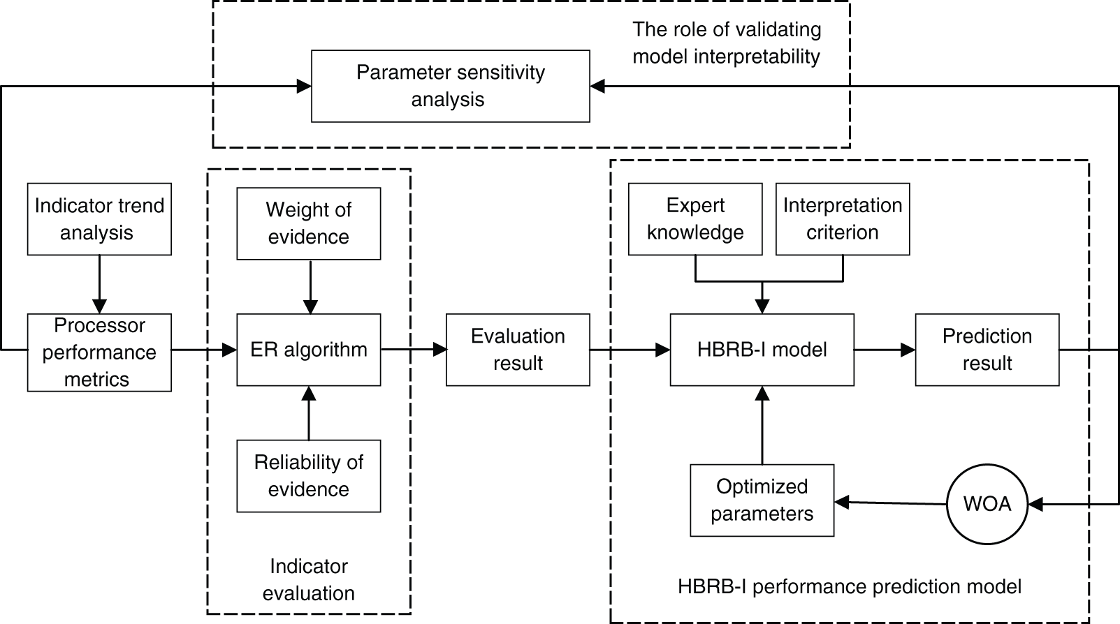
Figure 1: Flowchart of the structure of the model

3.1 Interpretability Definition of Predictive Models

As an expert system [21] developed from the if-then rule and the traditional D-S theory, BRB’s interpretability is constructed by general interpretable criteria. The HBRB performance prediction model can be divided into several sub-BRBs. Every sub-BRB needs an interpretable definition. They make up the interpretability of predictive models. As shown in Fig. 2, BRB consists of knowledge base and an inference engine. The knowledge base is derived from expert knowledge [22], and the ER inference engine is used to fuse the data. The interpretable criteria are specifically defined as follows:

(1) Integrity of input and output metrics

The integrity of the indicator data is conducive to the reasonable definition of the relationship between the indicators. According to the modeling causal attributes, the indicators can be divided into input indicators and output indicators. The difference between the input and output of the model will directly affect the accuracy of the results. For performance prediction models, at least one reference value should be set for each indicator, and at least one rule should be activated. Additionally, when performing rule reduction, it is necessary to ensure that each input corresponds to at least one rule [23]. Completeness is described as follows:

∀x∈U,∃ 1≤ξ≤M,aξ(x)>0∀x∈U,∃ 1≤k≤K,0<ωk≤1(4)

where the number of reference values for each indicator is M; the matching degree of the ξ-th reference value is expressed as aξ(x); U represents the entire feasible region of x; the number of belief rules is K; and ωk represents the activation weight of the rule.

(2) The rationality of rules

The rationality of rules is the basic requirement of model interpretability. Since the setting of the initial rules comes from expert knowledge, the rationality of rules is guaranteed. In addition, this criterion should also be satisfied when performing model optimization.

(3) Normativeness of rule matching degree

The matching degree of the rules represents the distribution characteristics of the indicators that affect the performance of the processor. To ensure the interpretability of the system distribution, the matching degree of each reference value in indicator space is normalized. Usually, the sum of the matching degrees of the reference values of each indicator data should be between [0,1], which is expressed as Eq. (28), which x~ represents the exact value of x:

∀ξ∈M,x∈U,0≤aξ(x)≤1,∑ξ=1maξ(x~)≤1(5)

(4) Structures and parameters have physical meaning

The overall structure and initial parameters of the model should have actual physical meaning. On the one hand, BRB is established by logical derivation. This conforms to the system principle. On the other hand, the initial parameters are dominated by belief rules. They include attribute weights, rule weights, activation weights, and beliefs [24].

a. Attribute weight: the importance of the premise attribute relative to other attributes

b. Rule weight: Indicates the importance of the rule relative to other rules

c. Activation weight: the degree to which the corresponding rule is activated by the input

d. Belief: how well the rules are converted into processor performance evaluation levels

(5) Distinguishability of the range of values

The input reference value of the model should be reasonably divided. The performance status evaluation level is represented by different level space ranges. There should be a distinction between different spatial ranges, so that different divisions of the corresponding meaning are different. It can help to meet the actual needs of the system.

(6) Normativeness of Information Transformation

Information conversion refers to the process of converting input and output information into belief distribution. To ensure the equivalence of the information conversion process is to maintain the characteristics of the original information. Yang et al. had developed a method to convert information based on rules and utility. This method could convert information reasonably and completely [25].

(7) Transparency of model inference

To maintain the interpretability of the rule base, BRB’s inference engine is required throughout the inference process. Besides, each reasoning process should be reasonably calculated and have an obvious causal relationship. This helps to ensure a clear description of the relationship between the input and output indicators. Based on the above conditions, the reliability of the model in practical applications can also be improved. As an inference engine for predicting model pairs, the ER algorithm can not only achieve clear inference and traceability of results, but also be able to explain itself.

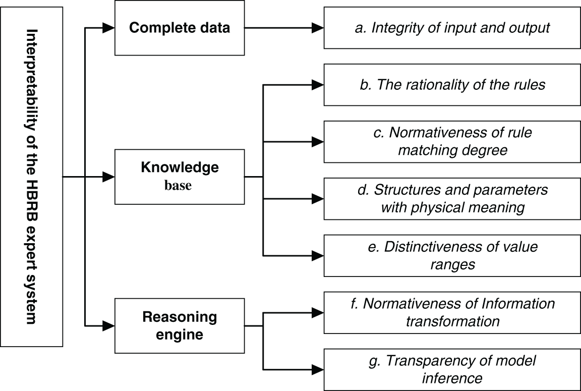
Figure 2: Diagram of the defining interpretable criterion

3.2 Performance Prediction Model Based on HBRB-I

In this section, the construction and optimization of the performance prediction model based on HBRB-I are defined and included as the following: (1) According to the mechanism analysis of the indicators, ER is used to evaluate the indicators; (2) Based on the evaluation results of the indicators, the HBRB model is constructed, and the detailed description and reasoning process of the prediction model are given; (3) Combined with WOA, a parameter optimization method is designed with interpretability constrained.

3.2.1 ER-Based Indicator Performance Evaluation

According to the mechanism analysis of the performance indicators, there may be correlations between indicators that affect the performance of the processor. If an indicator is analyzed individually in the process of performance evaluation. It is independent and unconvincing. In addition, the input and output index data in the process will be incomplete when indicators are blindly screened. Eventually, the evaluation results will produce errors. Therefore, it is proposed to use the ER algorithm to build the index evaluation model. The main implementation process is as follows, and Fig. 3 is the inference flow chart.

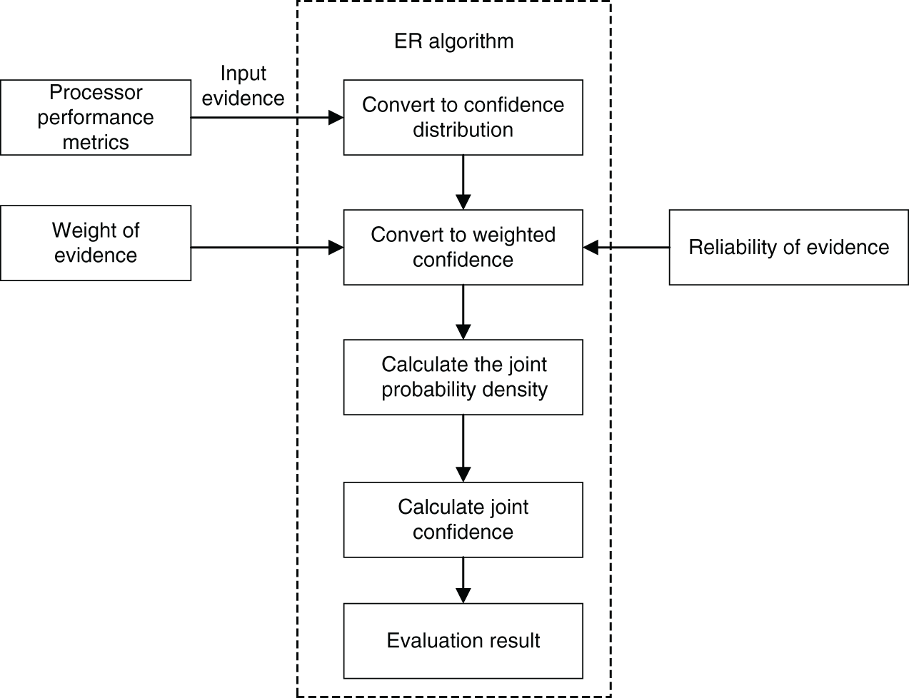
Figure 3: ER algorithm reasoning flow chart

Step 1: According to expert knowledge, the belief level of each performance index evaluation level is initialized, and the m-th metric is described as:

em={(Ar,σr,m),(ρ,σρ,m),r=1…R,m=1…M}(6)

where Ar is the evaluation level of the r-th indicator, and σr,m represents the belief to be assessed as grade Ar under evidence em. ρ is the global ignorance, and σρ,m represents unassigned belief.

Step 2: The ER iterative algorithm is used to calculate the basic probability quality of evidence, which is described by the following formula Eqs. (7)–(10):

mr,m=ωmρr,m(7)

mA,m=1−ωm∑r=1Rρr,m(8)

m¯A,m=1−ωm(9)

m~A,m=ωm(1−ωm∑r=1Rρr,m)(10)

where mr,m is the basic probability quality of the m-th evaluation level in the r-th indicator, ωm is the weight of the m-th indicator, m¯A,m represents the unassigned base probability mass, and m~A,m indicates the degree of incompleteness of the indicator.

Step 3: Dempster’s rule is used to solve the combined probability mass of evidence, and the reasoning process is described as follows:

mr,J(m+1)=FJ(m+1)[mr,J(m)mr,m+1+mr,J(m)mθ,m+1+mθ,J(m)mr,m+1](11)

mA,J(i)=m¯A,J(m)+m~A,J(m)(12)

m∼A,J(m+1)=FJ(m+1)[m∼A,J(m)m∼A,m+1+m∼A,J(m)m∼A,m+1+m∼A,J(m)m∼A,m+1](13)

m¯A,J(m+1)=FJ(m+1)[m¯A,J(m)m¯A,m+1](14)

FJ(m+1)=11−∑r=1R∑s=1Rmr,J(m)ms,m+1(15)

where mr,J(m),mr,J(m+1)=mr,m+1 represents the basic probability quality of the r+1-th index level after the r-th index is fused.

Step 4: The joint belief for evidence is calculated:

ρr=mr,J(M)1−m∼AJ(M)(16)

Step 5: If the utility of the evaluation level Ar is u(Ar). The expected utility value of the output y(k) is calculated as follows:

y(k)=∑r=1Ru(Ar)ρr(17)

3.2.2 Description and Reasoning of Performance Prediction Model Based on HBRB

As an expert system with the ER algorithm as the inference engine, the essence of BRB is a gray-box modeling type. Its system structure is composed of expert knowledge summarized by historical observation data and corresponding rules [26], so that the model itself has a certain interpretability. To build an interpretable HBRB expert system, expert knowledge should be embedded into the rules. However, the number of rules grows exponentially when the number of attributes increase. This leads to the combinatorial rule explosion problem [27]. To enhance the expansibility of BRB applications, starting from the system mechanism, a hierarchical HBRB model is constructed, which improves the modeling ability of BRBs. HBRB is composed of several sub-BRBs, which inherit the interpretability of BRBs. Additionally, each sub-BRB can perform information conversion, which effectively reduces the number of rules. Rule k is described as follows:

Rulekn:if y(1) is Z1e∧y(2) is Z2e… y(k) is ZSe, Then y is{(A1,β1,k),(A2,β2,k)…(AR,βR,k)},With rule weight θk,attribute weight δ1,δ2,…,δM in p1,p2,…,pm.(18)

where Rulekn(n=1,2,…,N) represents the k-th rule of the n-th subrule bas; k=1…K, K is the number of belief rules; Zie indicates the indicator input reference value (i=1,2,…,S); βr,k,r=1…R is the belief of the r-th in the k-th belief rule; Ar indicates the reference level of the output result; θk is the rule weight of the k-th belief rule; and δi represents the attribute weight.

The reasoning process of the HBRB model is mainly divided into five steps. First, expert knowledge is combined to convert the input value into the form of belief distribution. Second, the matching degree of the belief rules should be calculated. Finally, ER is used to obtain the output utility value.

Step 1: Expert knowledge is used to extract the initial parameters of the model, the parameter set of HBRB is described as:

ηn={θ1,…θk,β1,1…βR,K}(19)

Step 2: The matching degree of the belief rule is calculated:

ηkn={Aij+1−y(t)Aij+1−Aij,k=j(Aij≤y(k)≤Aij+1)y(t)−Aij+1Aij+1−Aij,k=j+10,k=1…K(k≠j andk≠j+1)(20)

where Aij+1 and Aij are the characteristic reference values in rules j+1 and j respectively.

Step 3: The activation weight of the rule is calculated. The calculation formula is shown in Eq. (21):

Wk=θkηk∑i=1Kθiηkk=1,…K(21)

where Wk represents the activation weight of the belief rule, θk represents the weight of rule k, and ηk represents the attribute weight.

Step 4: The belief of the performance index evaluation results is calculated based on ER analytical algorithm:

βr=φ×[∏k=1K(ωkβr,k+1−ωk∑i=1Rβi,k)−∏k=1K(1−ωk∑i=1Rβi,k)]1−φ×[∏k=1K1−ωk](22)

φ=[∑r=1R∏k=1K(ωkβr,k+1−ωk∑i=1Rβi,k)−(R−1)∏k=1K(1−ωk∑i=1Rβi,k)]−1(23)

where βr is the belief level of the r-th evaluation grade produced by the predictive model.

Step 5: According to the utility formula, the output result is described as Eq. (24):

yt=∑r=1RU(Ar)βr(24)

where yt is the actual output of the model and βr is the belief relative to the evaluation result Ar.

3.2.3 Parameter Optimization Based on the WOA

The parameters of the initial HBRB performance prediction model are derived from the actual system and expert knowledge. Considering the limited level of expert knowledge, it is difficult to accurately describe the performance state of the processor. Therefore, it is necessary to update the initial parameters of the model in conjunction with the optimization algorithm. In addition, the interpretability of the BRB will be destroyed in the process of parameter optimization. To ensure the interpretability and accuracy of the prediction model, interpretability constraints are added to the WOA algorithm. Therefore, the parameters with interpretability constraints are proposed. The model is shown in Fig. 4.

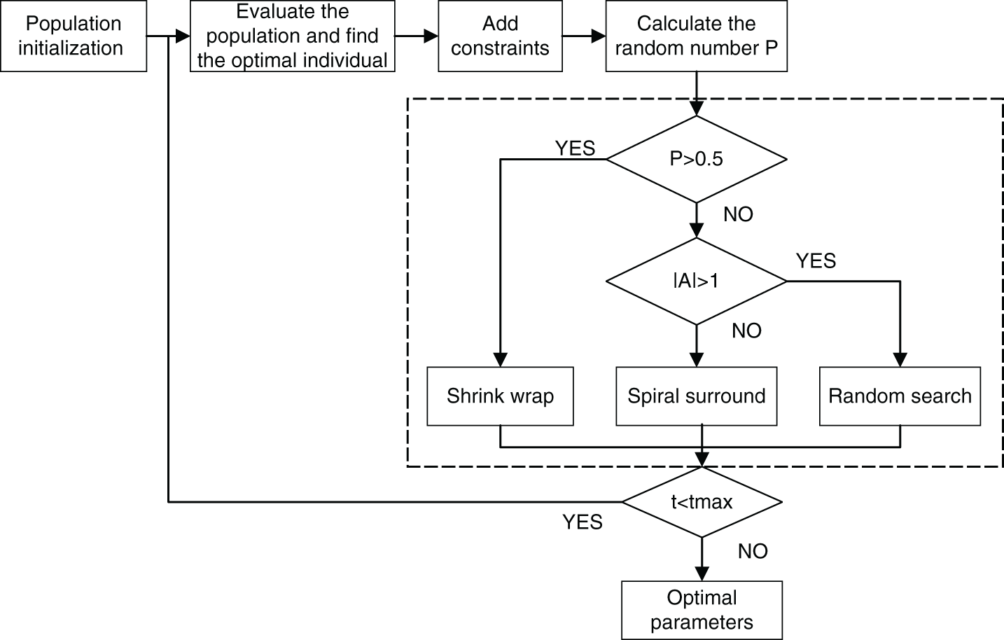
Figure 4: Flowchart of the WOA algorithm with interpretability constraints

First, the optimization objective function is given according to expert knowledge and the mean square error obtained from the actual training output, as shown in Eq. (25). MSE(⋅) represents the mean squared error. The actual output value is represented by yt, and the estimated output value is y⌢t, where the optimization objective and constraint conditions are shown in Eq. (26):

MSE(βr,k,ωk,θk)=1T∑t=1T(yt−y⌢t)2(25)

min MSE(βr,k,ωk,θk)in p1,p2s.t.:∑r=1Rβr,k=1,k=1,2,…,K,r=1,2,…,R0≤βr,k≤1,0≤ωk≤1,0≤θ1,θ2,…,θk≤1,k=1,2,…,K(26)

Based on the above analysis, the problem of BRB model optimization is a global optimization problem with constraints. As a metaheuristic optimization algorithm, the whale optimization algorithm is widely used in engineering [28]. The main advantages include the following: (1) A simple principle and fewer parameter settings. (2) A strong global search ability. (3) The ability to avoid local optimization [29]. The specific optimization process of the model is as follows:

Step 1: Population initialization. Assuming the population size is N, the number of iterations is t, and the search space is d-dimensional.

Step 2: The original method of scattering points is random and does not take full advantage of the interpretability of expert knowledge. For this problem, a solution space is formed with expert knowledge as the center, and points are randomly scattered in a certain area near the expert knowledge and set εi as the current optimum individual location:

εi=FK+(rand(N,d)−0.5)∗2(27)

where FK represents belief in expert knowledge.

Step 3: The constraint operation is added. The optimized belief rule deviates from the actual system. Conditional constraints should be added in the process of parameter optimization. It helps to satisfy the interpretability description of the model. Constraints are set in two ways.

Constraint 1: As a representation of processor performance characteristics and states, belief rules need to match the state of the actual system. However, the optimized rules generate errors that do not match the actual characteristics and do not satisfy the rationality of the rules in the interpretability definition. Therefore, constraints are added to the interval of regular distribution. It can be described as follows:

θk≤Fk(k=1,…,K),Fk∈{{θ1≤θ2≤…≤θN},{θ1≥θ2≥…≥θN},{θ1≤…≤max(θ1,θ2,…,)≥…≥θN}}(28)

where Fk is the interpretable constraint under rule k. Its value range is obtained with reference to the actual system. After filtering out conflicting belief levels, the final belief distribution shape is monotonic.

Constraint 2: Belief transformation of rules relies on expert knowledge, which can essentially meet actual system requirements. To ensure the reliability of the conversion process, the change in each belief rule cannot violate the expert knowledge. It is necessary to set a reasonable constraint range for the belief degree and select a belief distribution that meets the requirements:

θmin(p)≤θn,k≤θmax(p)(n=1,…,N,k=1,…,K)(29)

where θmin(p), θn,k, θmax(p) represents the minimum belief value set by the expert, the k-th belief value of the n-th rule, and the maximum belief value set by the expert.

Step 4: The whale group surrounds the current optimal individual, and the whale individual updates its position according to Eqs. (30)–(32):

D=∣C∗β∗t−βt∣(30)

βt+1=β∗t−AD(31)

A=2ar−aC=2ra=2−2ttmax(32)

The current number of iterations is represented by t; the coefficient vectors are A and C; the position vector of the current best solution is β∗t, which is updated in each iteration; and the position vector is written as βt. The scaling factor a decreases linearly throughout the bracketing process, decreasing from 2 to 0 in turn; the number of iterations at the current position is recorded as t; and the maximum number of iterations is recorded as tmax.

Step 5: In the prey stage, the whale group approaches the prey in a spiral pattern, and the update of each individual's own position is expressed as:

βt+1=exp⁡ (bl)cos⁡ (2πl)Dp+βt∗(33)

Dp=|βt∗−βt|(34)

where β∗(t) is the position of the optimal individual in the whale to the prey; b is constant; and l takes a random value [−1,1], which is a parameter to control the shape of the spiral.

Step 6: Searching for prey, the whale group searches for prey under the leadership of random individuals [30], the vector of the random individual position is denoted as βrand, and the searching process is shown in Eqs. (35) and (36):

D=∣Cβrand−βt∣(35)

βt+1=βrand−AD(36)

Remark 1: When evaluating the population to find the optimal individual, randomly scattering points in the expert knowledge area can make full use of the interpretability of expert knowledge. Before calculating the random number, constraints are added to the model. On the one hand, it satisfies the rationality of the belief rule and matches the characteristic state of the actual system. On the other hand, the expert knowledge won’t be violated by the change of the rules. During the hunting phase, the whale has a 50% chance to choose between the spiral mode and the shrinking circle mechanism to update its position. When |A| <= 1, the whale group shrinks to the prey under the leadership of the optimal individual. When |A| > 1, the whale group searches for the prey under the leadership of the random individual.

3.3 Global Sensitivity Analysis of Model Indicator Parameters

In the process of constructing the HBRB-I performance prediction model, the parameters of the model are derived from expert knowledge and the analysis results of input and output indicators. The expert knowledge is given according to the characteristics of the actual system and can be well explained by itself. The interpretability of the results of subjective index analysis needs to be further verified. Therefore, this section performs a global sensitivity analysis on the input and output metric parameters. Then the interpretability of the model derivation process is demonstrated.

The GSA considers the effect of the interaction between variables on the output when all parameters are changed at the same time. GSA mainly includes the regression analysis method, Morris-based screening method, Sobol method based on variance decomposition, and extended Fourier sensitivity test method [31]. Among the above methods, the variance-based Sobol method enables quantitatively analysis. Without special requirements for the analysis function, the uncertainty of input and output will be decomposed. Therefore, it has a wide range of applications [32]. Based on the Sobol method, indicator parameters are analyzed in the model. First, the model is decomposed into individual parameters and combined functions between parameters. Then, the influence of a single input parameter’s variance on the total output variance is calculated. Eventually, the importance of parameters and the interaction between parameters are analyzed. The steps are as follows:

First, the prediction model function f(x) is decomposed into a single model indicator parameter.

f(x1,x2,⋯,xk)=f0+∑i=1kfi(xi)+∑1≤i<j≤kkfij(xi,xj)+⋯+f1,2,⋯,k(x1,x2,⋯,xk)(37)

where xi represents different processor performance index parameters and f(x) expresses the relative performance of the output.

Based on the above conditions, the partial variance and the total variance are defined. The ratio of the partial variance to the total variance indicates the degree of the parameters’ influence and their interactions with the target response. The relationship between them can be expressed as:

D=∫Ωkf2(x)dx−f02(38)

Di1,i2,⋯,in=∫01⋯∫01fi1,i2,⋯,in2(xi1,xi2,⋯,xin)dxi1xi2⋯xin(n=1,2,⋯,k)(39)

D=∑i=1kDi+∑1≤i≺j≤kDij+⋯+D1,2,⋯,k(40)

where 1≤i1<⋯<in≤k, Di represents the variance produced by the independent action of the input indicator parameters. Dij represents the variance produced by the joint action of indicator parameters i and j. By analogy, the calculation formula of each first-order sensitivity is obtained.

Si1,i2,⋯,in=Di1,i2,⋯,inD(41)

where Si1,i2,⋯,in represents the sensitivity of each order of input parameters, and their sum constitutes the total sensitivity, which is calculated as:

STi=∑S(i)(42)

where STi indicates total sensitivity. Using the global sensitivity analysis method, the first-order sensitivity and total sensitivity of the performance indicators can be calculated. The larger the first-order sensitivity index of the index parameter is, the greater its impact on the relative performance of the output. If the total sensitivity index of a variable is small, it indicates that the change in the index parameter has a small impact on the output results. Besides, it also represents that there is a small interaction effect with other parameters in the index parameter [33]. According to the sorting of the total sensitivity index, the index parameter with the greatest impact on the performance of the processor can be found.

4  Case Study

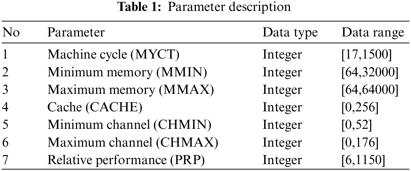
To verify the effectiveness of the proposed method, the computer hardware data of the UCI database is used as the main experimental data. The relative CPU performance data are obtained according to the description of processor cycle time and memory size. The data set contains 209 instances with a total of 7 attributes. The specific parameter descriptions are shown in Table 1.

4.1 Building the Performance Prediction Model

In this section, a processor performance prediction model based on the UCI computer hardware data set is built. Table 2 is a summary of the modeling steps, and Fig. 5 is a flow chart of the implementation of the performance prediction model.

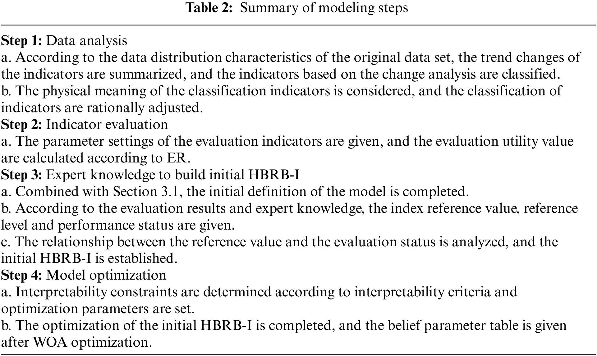
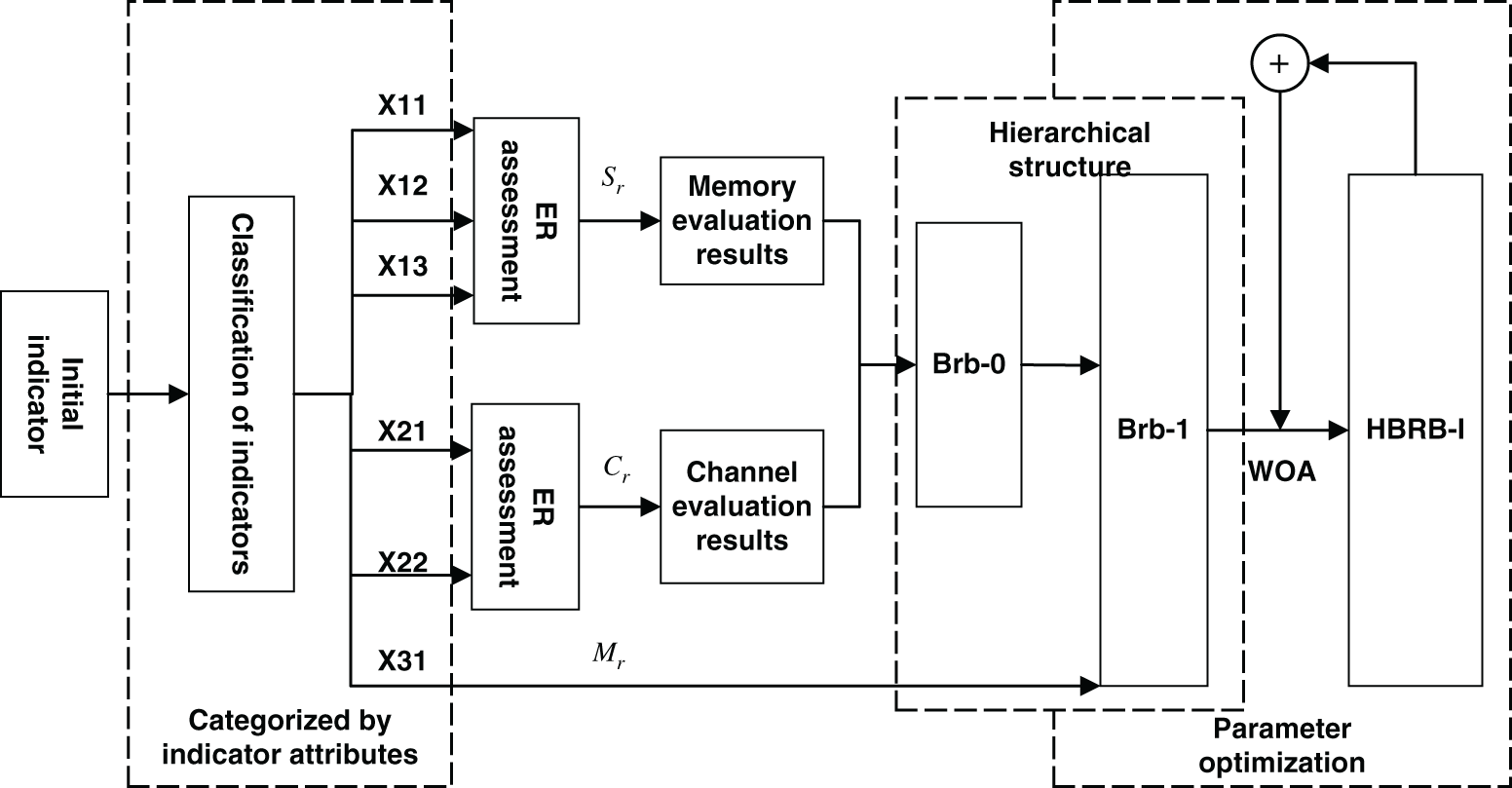
Figure 5: Performance prediction model implementation flow chart

4.1.1 Data Analysis

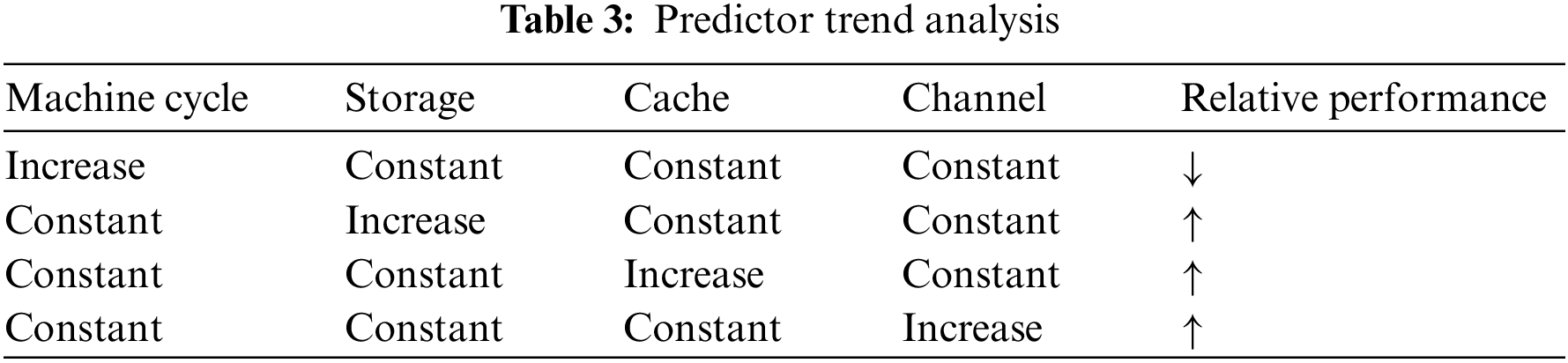
Combined with the change law of the actual value, the relationship between the processor indicators is analyzed. The forecast indicator trend analysis is shown in Table 3. According to the actual situation, the larger the machine cache, the higher the data processing efficiency. The ability to execute programs concurrently becomes stronger as the number of channels increases. In addition, the operation per unit time is completed faster when the machine cycle becomes shorter. Therefore, the improvement of these factors would lead to the improvement of processor performance. According to the index trend change relationship and physical meaning, the performance influencing factors can be divided into three categories: storage, channel, and machine cycle. Storage includes minimum memory, maximum memory, and cache, while channel includes minimum channel and maximum channel.

4.1.2 Evaluation of Indicators

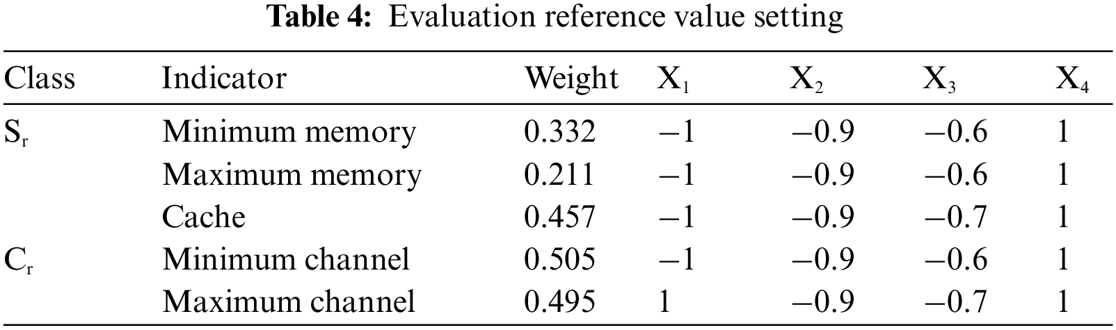
Based on the above index classification results, the ER algorithm is used for index evaluation. The reference values are set as shown in Table 4. Each index is set with 4 reference values, corresponding to (x1, excellent), (x2, good), (x3, middle) and (x4, poor); regardless of the reliability of the evidence, the sum of the weights of the indicators of the same category is 1. Assuming that Sr and Cr are used to express the evaluation results of storage factors and channel factors, Mr represents MYCT.

4.1.3 Expert Knowledge to Establish Initial HBRB-I

Based on the above analysis, the initial HBRB-I establishes a belief rule, which is expressed as follows:

if Sr is Z1e∧Cr is Z2e,Then result is {(A1,β1,k),(A2,β2,k)…(A4,β4,k)},With rule weight θk,attribute weight δ1,δ2, in p1,p2,…,pm.(43)

where Sr is the estimated utility value of the storage factor, Cr indicates the estimated utility value of the channel factor, and A represents the level of processor performance state, which can be described by Very Small (VS), Small (S), Middle (M), and Large (L). The performance status reference values are shown in Table 5.

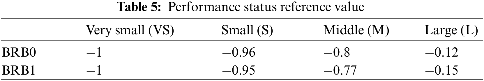
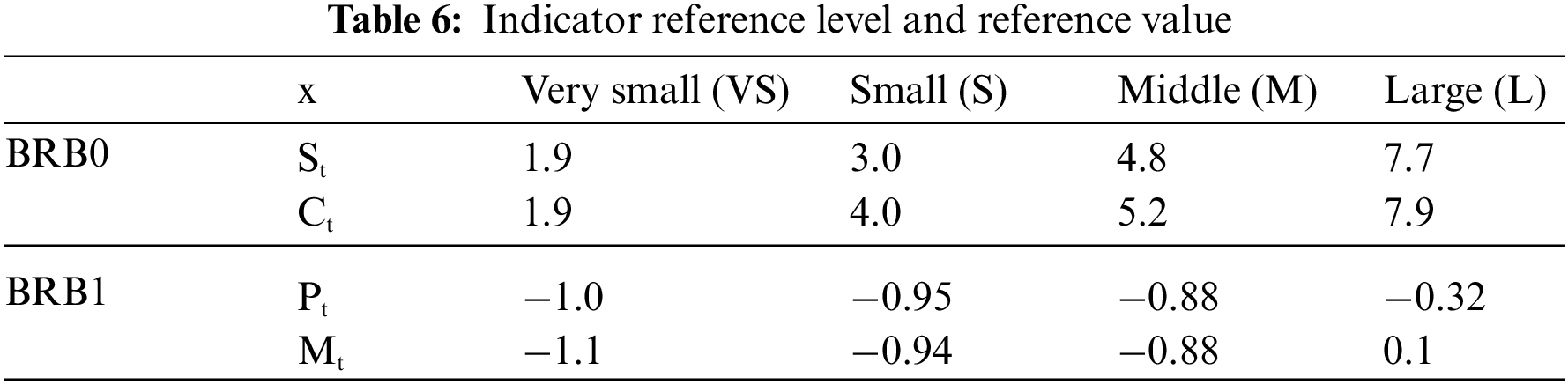
To avoid the problem of rule combination explosion, an interpretable hierarchical BRB performance prediction model is constructed. According to the reasoning process shown in Table 6, the model structure is divided into two layers. First, the evaluation results St and Ct of the storage factor and channel factor are used as the input of the first layer BRB0, the initial belief and interpretability constraints are set in combination with expert knowledge, and the index reference level and reference value are given. Second, the output result Pr of BRB0 and MYCT Mr are combined as the input of the second layer BRB1. The initial confidence rules and reference values are set, and the performance prediction results are obtained by continuous training. The index reference value settings are shown in Table 6. Each index has 4 reference values, and 16 rules are activated, which conform to the input and output integrity in the definition of interpretability. The range of values can be distinguished. Both rule weights and attribute weights are set to the constant 1. According to the normative requirements of the rules’ matching degree in the interpretability definition, the sum of the matching degree of the input data is limited between [0, 1].

4.1.4 Model Optimization

Considering the limitations of expert knowledge, the prediction of the performance state by the initial model is not sufficiently accurate [34]. Therefore, it is necessary to use the optimization algorithm to update the initial parameters to improve the accuracy of the model. In this paper, the parameters are optimized based on the WOA. The number of training iterations is 600, the optimization dimension is 82, the population size is 25, the training set is 209 data, and the test set is 100 data.

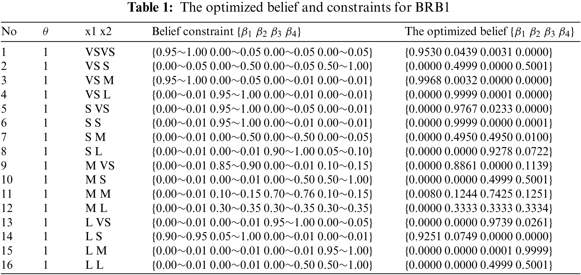
Taking the initial parameters of BRB1 as an example, the belief constraints and the optimized belief are shown in Appendix A Table 1.

4.2 The Process of Parameter Sensitivity Analysis

To verify the model interpretability, based on the HBRB-I performance prediction model, Sobol global sensitivity analysis of parameters is performed. The specific process can be described as follows:

Step 1: Select the performance index parameters input by the model as independent variables, and the relative performance values predicted by the output model are used as the dependent variable.

Step 2: According to the statistical distribution of the index parameters, the value range of each parameter is determined, please refer to Table 1.

Step 3: The index parameters are randomly sampled using the Latin hypercube sampling method [35], and N sets of training samples are generated as input variables.

Step 4: The resulting set of training samples is used to input the surrogate model [36], the sensitivity analysis data are obtained by training, and the results are shown in Table 7.

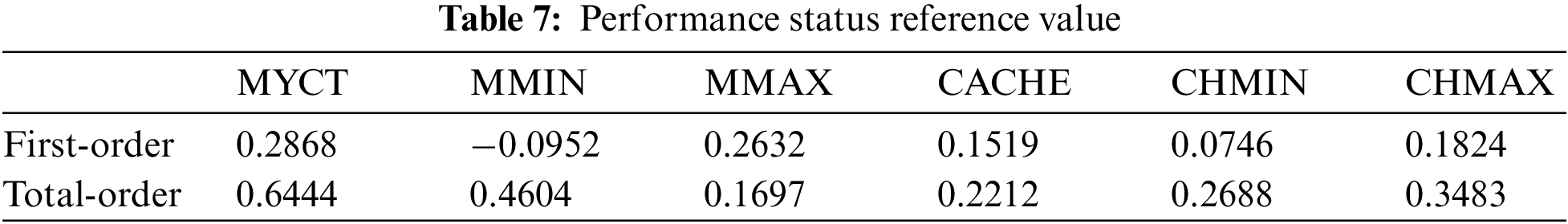
Comparing the values of different sensitivities of performance parameters, it is found that the total sensitivity of the machine is significantly higher than other parameters. The first-order sensitivity is generally smaller than the total sensitivity value. The result indicates that a single index parameter has a small impact on the processor performance. The interaction between each index has a great impact on the performance.

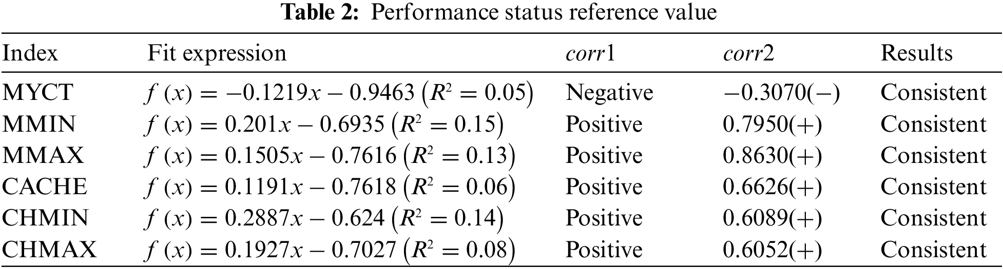
To further explore how each index parameter affected the performance model, the linear fitting method is used to fit the functional relationship expression between the predicted performance value and single index parameter. This helps to study the correlation between the index parameter and the performance. Assuming that the index parameters are uniform linearly, distributed within the range during the fitting process, other parameters are averaged. The HBRB-I model is used to obtain the performance prediction value. In addition, the correlation coefficient between each index parameter of the original data set and the relative performance is calculated as corr1. The correlation between the performance prediction value and the index parameter in the linear fitting expression is represented as corr2. R2 is used to reflect the degree of linear fit. The correlation coefficient expression is shown in Eq. (35) and correlation comparison results are shown as in Appendix B Table 2.

r=∑i=1n(xi−x¯)(yi−y¯)∑i=1n(xi−x¯)2∑i=1n(yi−y¯)2(44)

where xi is the indicator parameter, x¯ represents the mean value of each parameter, yi is the actual relative performance value, and y¯ is the value of the predicted performance.

According to the experimental results, the correlation coefficient corr2 of minimum memory, maximum memory, and minimum channel have higher sensitivity than that of other parameters. The result indicates that the effect of these indicators on performance is less affected by changes in other parameters. Moreover, its influence is greater than other parameters. In addition, except for the machine cycle, which is negatively correlated, the other parameters are positively correlated with the prediction performance. The correlation between the index parameters and performance in the HBRB-I model is basically consistent with the original data, which verifies that this interpretable modeling method can maintain the relationship between input and output metrics. Therefore, the HBRB-I performance prediction model not only improves the comprehensibility of the model, but also ensures a stable changing relationship between each input index and the predicted output. This is in line with the actual operating principle of the system.

4.3 Analysis of Case Experiment Results

In this section, the accuracy and interpretability of the model are mainly compared. The experimental results are combined to prove the effectiveness of the method.

4.3.1 Model Accuracy Analysis

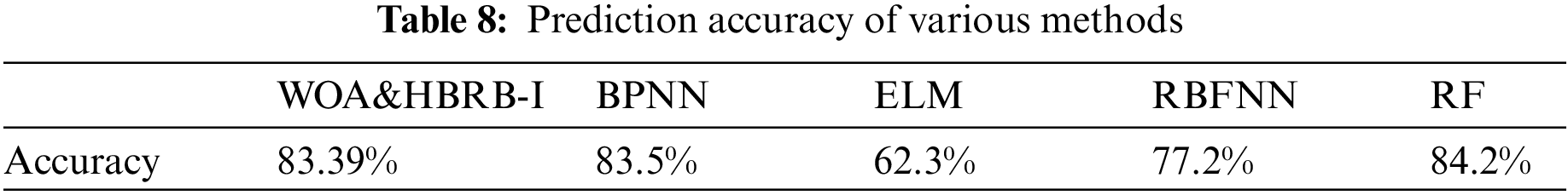
To verify the effectiveness of the method, the method proposed in this paper is horizontally compared with four types of machine learning methods. They are backpropagation network (BPNN), radial basis function neural network (RBFNN), extreme learning machine (ELM) and random forests (RF). For comparison, each method uses the same number of training and test sets, and conducts 10 rounds of experiments. The fitting effect is shown in Fig. 6. The square error value of the HBRB-I model is maintained between 0.004–0.006, which also maintains good accuracy compared to other machine learning algorithms. Table 8 shows the prediction accuracy of various methods.

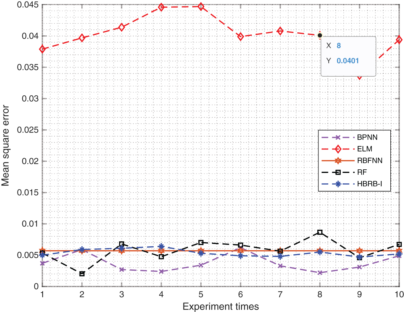
Figure 6: MSE values of different methods

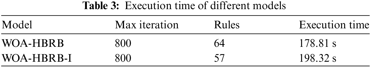
To better evaluate the performance of the proposed algorithm, the computation time and convergence of the proposed method are discussed. As shown in Fig. 7, the convergence speed of WOA&HBRB-I is faster, the starting point of optimization is closer to the optimal solution, and the overall convergence of the model is better. However, in terms of execution time, as shown in Appendix B Table 3. WOA&HBRB-I takes longer time, and the reasons can be explained as follows. On the one hand, WOA&HBRB-I reduces redundant rules in the model and the complexity of the model. It also improves the optimization process. Thus, the convergence speed of the model increased. On the other hand, the optimization process based on interpretability constraints screens out the rules that have a greater impact on the system and take more computation time. Therefore, it shows longer execution time.

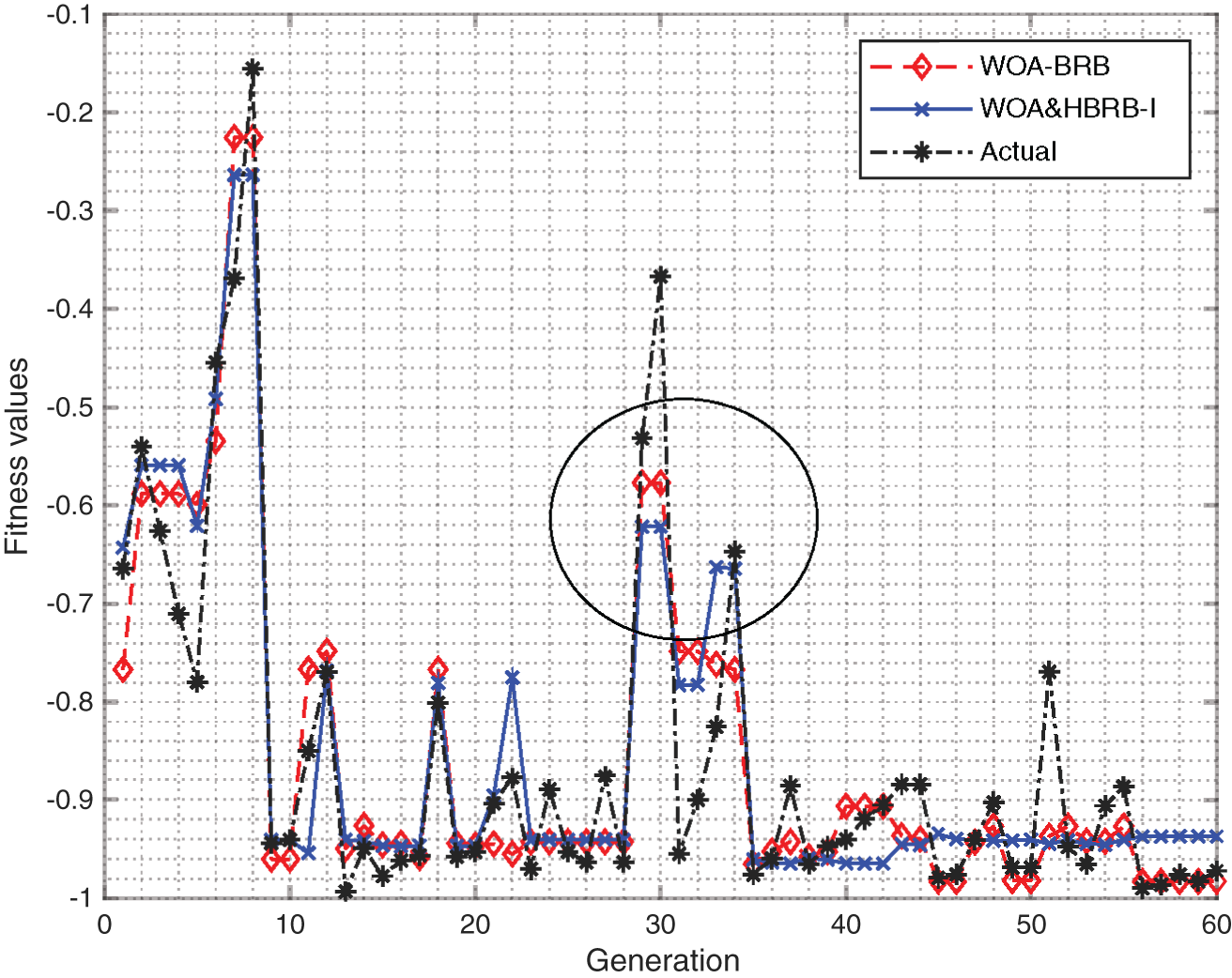
Figure 7: Fitness values of different models

4.3.2 Model Interpretability Analysis

The belief distribution of each rule is shown in Fig. 8. The belief distribution of the HBRB-I model is basically the same as the rule distribution given by the expert knowledge. The green curve represents expert knowledge. The blue curve represents the belief distribution of the HBRB model without adding an interpretable definition. The red curve represents the belief distribution of the HBRB-I model. Comparing the belief distribution of HBRB and expert knowledge, some rule’s judgments are quite different. This means that the rules are missing or wrong, and it is verified that the model adds interpretability constraints to improve the effective use of expert knowledge. Therefore, the HBRB-I model is more interpretable under the premise of having similar prediction effects.

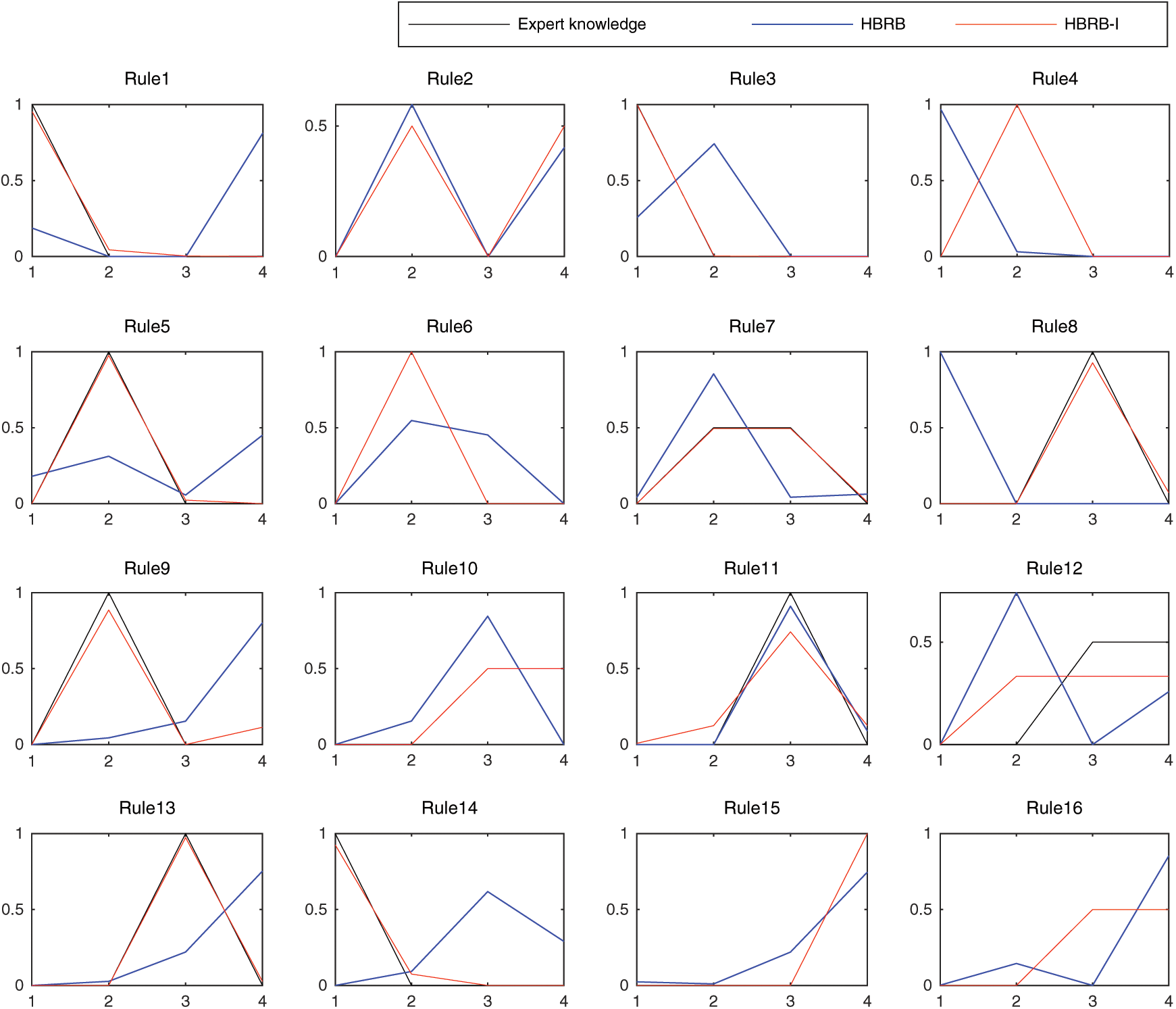
Figure 8: Contrast chart of belief distributions for BRB1

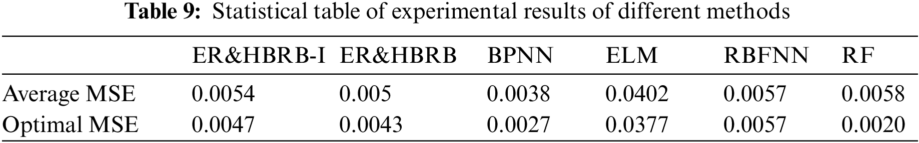
Table 9 shows the average MSE value and optimal MSE value of different methods. The following conclusions can be drawn from analyzing the experimental results:

(1)   Although the accuracy of the HBRB-I model is slightly different from that of machine learning algorithms such as BPNN, ELM, and RF, the HBRB-I model is interpretable and the reasoning process can be retroactive. As for data-driven modeling methods such as BPNN, ELM, and RF, the internal structure is invisible. The inference engine ER deduction is used in HBRB-I. It could reasonably explain the causal relationship between input and output to make the conclusion more reliable. Besides, the HBRB-I model can make full use of expert knowledge to characterize the system and help users better understand the model structure. However, they cannot be achieved by ordinary machine learning methods.

(2)   Compared with the HBRB model without interpretable definition, the HBRB-I model has no obvious difference in accuracy, and its advantage is reflected in the interpretability. On the one hand, the optimization method of the HBRB-I model has interpretability constraints. When the WOA is initialized, the optimal individual is selected based on expert knowledge instead of random selection in the HBRB model, which effectively utilizes expert knowledge. The rationality of the optimal individual selection is improved. On the other hand, the rule matching degree of the HBRB-I model sets a screening interval. Therefore, the belief distribution of the model satisfies the actual performance prediction system. The HBRB fails to solve the problem of reasonable belief distribution, such as the 14-th rules in Fig. 7. The judgements of “very small” and “small” in the belief level of the HBRB model are inconsistent. The belief level distribution of the HBRB-I model is basically consistent with the expert knowledge. It shows the role of the interpretability of the HBRB-I model.

5  Conclusion

This paper proposes a processor performance prediction method based on sensitivity analysis and an interpretable hierarchical belief rule base. Transparent reasoning engine is used in the model reasoning process to deduce the problem. Besides, the interpretability criterion is added to make full use of the characteristics of the expert knowledge description system. It can solve the problems of ineffective use of expert knowledge and unreasonable belief optimization. Therefore, the performance prediction method proposed in this paper has strong interpretability. The results of predictive model are traceable. The relationship between input and output also verifies the role of interpretable modeling. Compared with other methods, the interpretability enhances the reliability of the system under the condition that the accuracy is basically guaranteed.

Acknowledgement: The researchers would like to thank Harbin Normal University for funding this project.

Funding Statement: This work is supported in part by the Postdoctoral Science Foundation of China under Grant No. 2020M683736, in part by the Teaching reform project of higher education in Heilongjiang Province under Grant No. SJGY20210456, and in part by the Natural Science Foundation of Heilongjiang Province of China under Grant No. LH2021F038.

Conflicts of Interest: The authors declare that they have no conflicts of interest to report regarding the present study.

A Appendix

Appendix A

Appendix B

References

1. B. Li, P. Lu and B. Ramadass, “Accurate and efficient processor performance prediction via regression tree-based modeling,” Journal of Systems Architecture, vol. 55, no. 10–12, pp. 457–467, 2009. [Google Scholar]
2. G. Inal and G. Kucuk, “Application of machine learning techniques on prediction of future processor performance,” in 2018 Sixth Int. Symp. on Computing and Networking Workshops (CANDARW), Takayama, Japan, pp. 190–195, 2018. [Google Scholar]
3. Z. J. Zhou, Y. Cao, G. Y. Hu, Y. M. Zhang, S. W. Tang et al., “New health-state assessment model based on belief rule base with interpretability,” Science China Information Sciences, vol. 64, no. 7, pp. 1–15, 2021. [Google Scholar]
4. C. Zheng and Y. Jiong, “Performance prediction based on random forest for the stream processing checkpoint,” Journal of Electronics & Information Technology, vol. 42, no. 6, pp. 1452–1459, 2020. [Google Scholar]
5. V. Maurya and S. C. Gupta, “Comparative analysis of processors performance using ANN,” in 2015 5th Int. Conf. on IT Convergence and Security (ICITCS), Kuala Lumpur, Malaysia, pp. 1–5, 2015. [Google Scholar]
6. D. Feng, “Coupled-least-squares identification for multivariable systems,” IET Control Theory & Applications, vol. 7, no. 1, pp. 68–79, 2013. [Google Scholar]
7. B. Kamiński, M. Jakubczyk and P. Szufel, “A framework for sensitivity analysis of decision trees,” Central European Journal of Operations Research, vol. 26, no. 1, pp. 135–159, 2018. [Google Scholar]
8. S. Sachan, F. Almaghrabi, J. B. Yang and D. L. Xu, “Evidential reasoning for preprocessing uncertain categorical data for trustworthy decisions: An application on healthcare and finance,” Expert Systems with Applications, vol. 185, no. 2, pp. 115597, 2021. [Google Scholar]
9. J. B. Yang and D. L. Xu, “Evidential reasoning rule for evidence combination,” Artificial Intelligence, vol. 205, no. 1, pp. 1–29, 2013. [Google Scholar]
10. Y. P. Wen, Y. Wang, J. X. Liu, B. Cao and Q. Fu, “CPU usage prediction for cloud resource provisioning based on deep belief network and particle swarm optimization,” Concurrency Computation Practice and Experience, vol. 32, no. 14, pp. e5730, 2020. [Google Scholar]
11. Z. J. Zhou, G. U. Hu, B. C. Zhang, C. H. Hu, Z. G. Zhou et al., “A model for hidden behavior prediction of complex systems based on belief rule base and power set,” IEEE Transactions on Systems, Man, and Cybernetics: Systems, vol. 48, no. 9, pp. 1–7, 2017. [Google Scholar]
12. C. H. Hu, Z. C. Feng, Z. J. Zhou, G. Y. Hu and W. He, “Structural safety assessment method for liquid launch vehicles considering environmental interference,” Science in China: Information Science, vol. 50, no. 10, pp. 1559–1573, 2020. [Google Scholar]
13. Y. Gao, X. Liu and J. Xiang, “FEM simulation-based generative adversarial networks to detect bearing faults,” IEEE Transactions on Industrial Informatics, vol. 7, no. 16, pp. 4961–4971, 2020. [Google Scholar]
14. X. H. Dong, Z. J. Zhou, C. H. Hu, Z. C. Feng and Y. Cao, “Performance evaluation method of inertial navigation system based on hierarchical belief rule base,” Journal of Aeronautics and Astronautics, vol. 42, no. 7, pp. 441–451, 2021. [Google Scholar]
15. Y. Cao, Z. J. Zhou, G. Y. Hu, C. H. Hu, S. W. Tang et al., “A new multilayer belief rule base model for complex system modeling,” IEEE Systems Journal, vol. 16, no. 3, pp. 4301–4312, 2021. [Google Scholar]
16. Y. Cao, Z. J. Zhou, C. H. Hu, W. He and S. W. Tang, “On the interpretability of belief rule based expert systems,” IEEE transactions on Fuzzy Systems, vol. 29, no. 11, pp. 3489–3503, 2021. [Google Scholar]
17. Z. J. Zhou, Y. Cao, C. H. Hu, S. W. Tang, C. C. Zhang et al., “Interpretability and development of rule-based modeling methods,” Chinese Journal of Automation, vol. 47, no. 6, pp. 1201–1216, 2021. [Google Scholar]
18. P. Carsten, “Local reliability-based sensitivity analysis with the moving particles method,” Reliability Engineering & System Safety, vol. 207, no. 7, pp. 107269, 2021. [Google Scholar]
19. P. Zhang, “A novel feature selection method based on global sensitivity analysis with application in machine learning-based prediction model,” Applied Soft Computing, vol. 85, pp. 105859, 2019. [Google Scholar]
20. L. H. Yang, J. Liu, Y. M. Wang and L. Martínez, “New activation weight calculation and parameter optimization for extended belief rule-based system based on sensitivity analysis,” Knowledge and Information Systems, vol. 60, no. 2, pp. 837–878, 2019. [Google Scholar]
21. X. Wu, D. H. Wang, W. H. Cao and M. Ding, “A genetic-algorithm support vector machine and D-S evidence theory based fault diagnostic model for transmission line,” IEEE Transactions on Power Systems, vol. 34, no. 6, pp. 4186–4194, 2019. [Google Scholar]
22. Z. J. Zhou, G. Y. Hu, C. H. Hu, C. L. Wen and L. L. Chang, “A survey of belief rule-base expert system,” IEEE Transactions on Systems, Man, and Cybernetics: Systems, vol. 51, no. 8, pp. 4944–4958, 2021. [Google Scholar]
23. L. L. Chang, Z. J. Zhou and H. Liao, “Generic disjunctive belief rule base modeling, inferencing, and optimization,” IEEE Transactions on Fuzzy Systems, vol. 27, no. 9, pp. 1866–1880, 2019. [Google Scholar]
24. Z. J. Zhou, L. L. Chang and C. H. Hu, “A new BRB-ER-based model for assessing the lives of products using both failure data and expert knowledge,” IEEE Transactions on Systems, Man, and Cybernetics: Systems, vol. 46, no. 11, pp. 1529–1543, 2016. [Google Scholar]
25. J. B. Yang, J. Liu, J. Wang, H. S. Sii and H. W. Wang, “Belief rule-base inference methodology using the evidential reasoning approach-RIMER,” IEEE Transactions on Systems, Man, and Cybernetics: Systems, vol. 36, no. 2, pp. 266–285, 2006. [Google Scholar]
26. Z. C. Feng, W. He, Z. J. Zhou, X. J. Ban, C. H. Hu et al., “A new safety assessment method based on belief rule base with attribute reliability,” IEEE/CAA Journal of Automatica SINICA, vol. 8, no. 11, pp. 1774–1785, 2021. [Google Scholar]
27. S. S. Liu, H. L. Zhu, X. X. Han, Q. Q. Mu and W. He, “Enterprise risk assessment model based on principal component regression and hierarchical belief rule base,” Computer Science, vol. 48, no. 2, pp. 570–575, 2021. [Google Scholar]
28. M. Seyedali and L. Andrew, “The whale optimization algorithm,” Advances in Engineering Software, vol. 95, no. 12, pp. 51–67, 2016. [Google Scholar]
29. I. Aljarah, H. Faris and S. Mirjalili, “Optimizing connection weights in neural networks using the whale optimization algorithm,” Soft Computing, vol. 22, no. 1, pp. 1–15, 2018. [Google Scholar]
30. A. Brodzicki, M. Piekarski and J. Jaworek-Korjakowska, “The whale optimization algorithm approach for deep neural networks,” Sensors, vol. 21, no. 23, pp. 8003, 2021. [Google Scholar]
31. X. Dong and D. P. Zhang, “Global sensitivity analysis of weapon equipment combats effectiveness based on extreme learning machine,” Computer and Modernization, no. 5, pp. 86–92, 2018. [Google Scholar]
32. C. J. Lin, X. D. Yang, Y. J. Gong, W. T. Ding, X. D. Cheng et al., “PSO-BP-based earth pressure shield earth silo pressure prediction model and sensitivity analysis of tunneling parameters,” Journal of Applied Basic and Engineering Sciences, vol. 29, no. 5, pp. 1220–1233, 2021. [Google Scholar]
33. K. Sergei, F. Balazs, S. Nilay and M. Wolfgang, “The identification of model effective dimensions using global sensitivity analysis,” Reliability Engineering & System Safety, vol. 96, no. 4, pp. 440–449, 2011. [Google Scholar]
34. Z. C. Feng, Z. J. Zhou, C. H. Hu, L. L. Chang, G. Y. Hu et al., “A new belief rule base model with attribute reliability,” IEEE Transactions on Fuzzy Systems, vol. 27, no. 5, pp. 903–916, 2019. [Google Scholar]
35. W. F. Zhang, Y. B. Che and Y. S. Liu, “Improved latin hypercube sampling method in power system reliability assessment,” Automation of Electric Power Systems, vol. 39, no. 4, pp. 52–57, 2015. [Google Scholar]
36. Y. Zhang, W. G. Zhang, T. Ma and T. Tang, “Optimal design method for complex nonlinear systems based on global sensitivity analysis and dynamic surrogate model,” Chinese Journal of Mechanical Engineering, vol. 51, no. 4, pp. 126–131, 2015. [Google Scholar]
A Appendix
Appendix B
Cite This Article
Copyright © 2023 The Author(s). Published by Tech Science Press.
This work is licensed under a Creative Commons Attribution 4.0 International License , which permits unrestricted use, distribution, and reproduction in any medium, provided the original work is properly cited.
Downloads
Citation Tools