Lung Cancer Segmentation with Three-Parameter Logistic Type Distribution Model

1  Introduction

Lung cancer is the leading cause of mortality in the world [1], affecting both men and women equally. According to the American Cancer Society, 222,500 [2] new instances of lung cancer were diagnosed in 2020 and 155,870 individuals died as a result of the disease. The survival rate for colon cancer is 65.4%, whereas breast cancer has a survival rate of 90.35% and prostate cancer has a survival rate of 99.6% which is much lower than the overall survival rate of 65.4% [3]. It is possible that a lung nodule is an indication of lung cancer. Only 16% of cases are discovered in the early stages. If these nodules are discovered while they are still in their original location, the odds of survival increase from 10% to 65%–70%. Lung cancer is detected and treated with the use of imaging methods such as Multidetector X-ray Computed Tomography (MDCT) was shown in the Fig. 1. If you have a CT scanning [4] today, you will get a large amount of information. Performing all of this data segmentation and analysis by hand is difficult and time-consuming. It makes the work of the radiologist more complicated and time-consuming. It is possible that glancing at a large number of images can increase the likelihood of missing essential clinical criteria such as abnormalities.

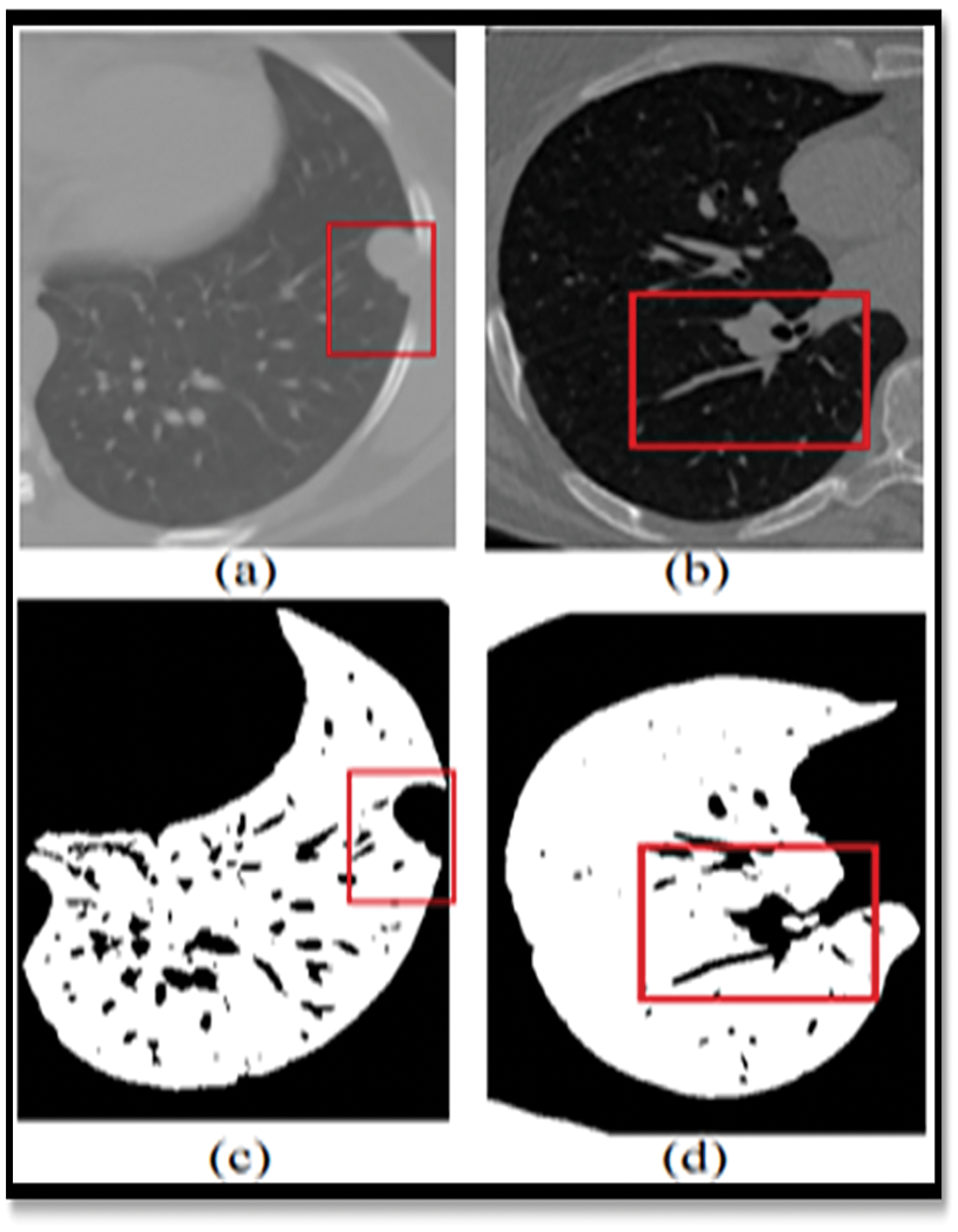
Figure 1: Showing the limitations of the normal image-based segmentation

In order to address this issue, Computer-Assisted Diagnosis (CADx) and Computer-Assisted Detection (CADe) have been investigated as potential methods of assisting radiologists [5] with CT scans while also improving their diagnostic accuracy. For the last two decades, researchers from all around the globe have been focusing their efforts on strategies to increase the accuracy of lung nodule detection. The four major components of the CAD/CADe system are shown in Fig. 1. (1) The lungs are immediately divided into two halves. Selection of nodule candidates or division of nodules are two examples of nodule division. 3-Nodules and the many forms of nodules 4) It was discovered that the patient had lung cancer.

For lung segmentation, there are two primary goals: to reduce the amount of time it takes to do the calculations, and to ensure that a search only goes to the lung parenchyma [6] by making sure the boundaries are extremely well defined. There have been several reports of various methods of dividing the lung, but only a handful of them have been shown to involve juxta pleural nodules [7]. During the second stage of the construction process, basic image processing methods are used to identify a variety of nodules in the lung area that has been successfully healed. The final step makes use of machine learning to determine which objects include nodules and which ones do not contain nodules [8] (e.g., segments of airways, arteries, or other non-cancerous lesions). The Major Contributions of the proposed research work are as follows:

•   To develop the algorithm for lung segmentation and lobe volume quantification.

•   To develop automatic segmentation of lungs field with various abnormal patterns attached to lung boundary such as excavated mass, pleural nodule, etc.

•   To design the lung segmentation algorithm for the inclusion of juxta pleural nodules and pulmonary vessels.

•   To design the algorithm for segmentation of various types and shapes of pulmonary nodules.

2  Related Works

Convolutional neural networks are used in the creation of U-NET [9]. Despite the fact that this network has just 23 layers still it performs well. Although it is not as difficult as networks with hundreds of layers, it nevertheless requires a significant amount of effort. Down-and up-sampling are used extensively in a single network environment. Deconvolution is used to make the map of features more visible by removing some of the details. Depending on where you reside, this is referred to as a decoder or an encoder. If you utilize a convolution or pooling layer [10], you will obtain feature maps that include varying amounts of information from the images with which they are merged, depending on the layer you select. This is done in order to recover the abstract data that has been lost and to enhance network segmentation and segmentation accuracy.

When all of the aforementioned problems are taken into consideration, it is critical to establish temporary U-NET networks in order to improve the situation even more. Why there hasn’t been enough study on how to discover lung cancer nodules that have been divided into segments is explained in Table 1.

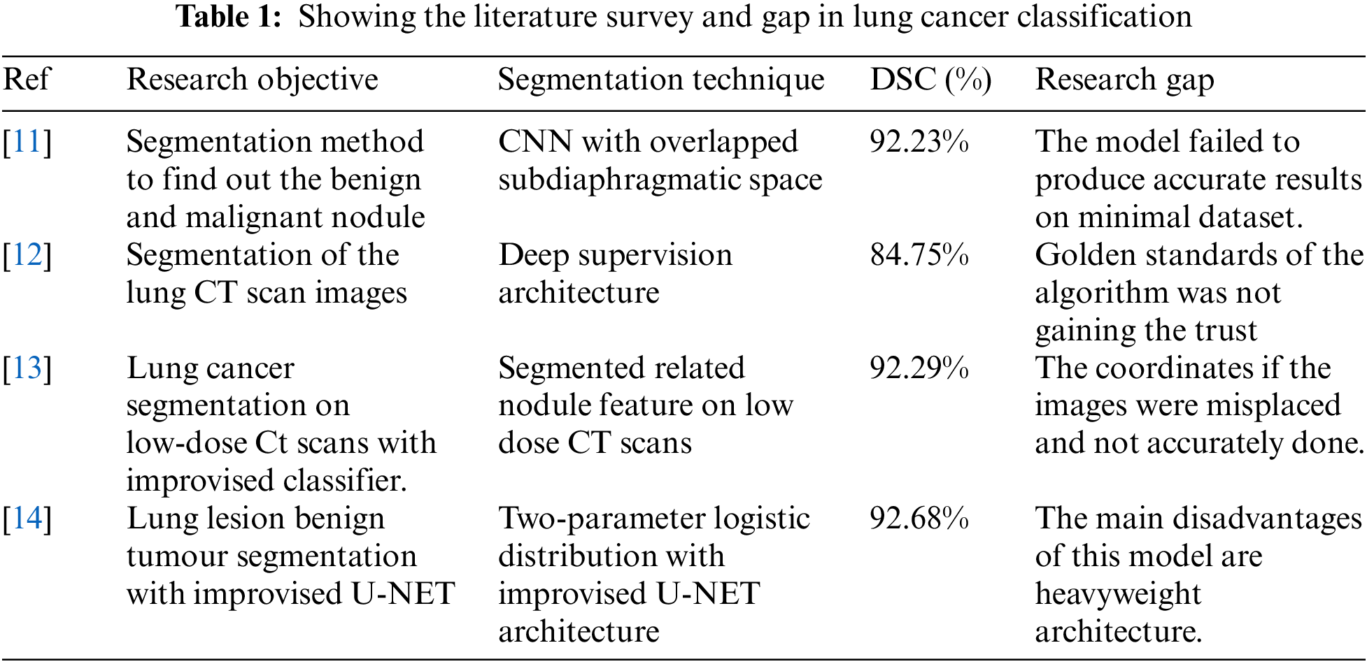
Researchers from [11–14] used the identical data set, but the model’s robustness was degraded. Because the U-NET could not be utilized with new data types, the IOU intersection and dice co-efficient index accuracy were unavailable. This concept enhances the efficiency of fully linked and multiscale conversion systems. The previous models had the following main flaws. Gradient’s descent fades away as one moves farther from the network’s error computation and training data output. Weakly evolving intermediate stratum models may opt to skip using abstract layers altogether. The Following research questions was not addressed properly. They are listed as follows:-

The U-Net architecture cannot extract information from it. It seems that the suggested U-NET Architecture and Three Parameter Logistic Type Distribution Models’ benefits outweigh any disadvantages produced by their intermediary layers’ fewer steep slopes. These experiments found that U-NET Architecture and Three Parameter Logistic Type Distribution outperform other designs at recognising small items in pictures. Modelling models that aren’t similar or that include new technology is straightforward and quick. To correctly distribute light, orientation, and components, an algorithm may need to recognise the same item again on a very small scale. Convolutional networks may be able to gain these traits without giving up any of their existing knowledge. However, when compared to other previously evaluated models, DB-NET outperformed them with more data. The LUNA16 benchmark dataset gave us a wide range of data to examine our model.

3  Proposed Methodologies

The proposed methodology section consists of the overall proposed methodology. A three-parameter logistic distribution is proposed in this work. The details of the applied methodology are given below.

3.1 U-NET Semantic Segmentation

The U-Net architecture was shown in the Fig. 2, built upon the fully convolutional network [15], has proven to be effective in biomedical image segmentation. However, U-Net applies to skip connections to merge semantically different low-and high-level convolutional features, resulting in not only blurred feature maps but also over-and under-segmented target regions.

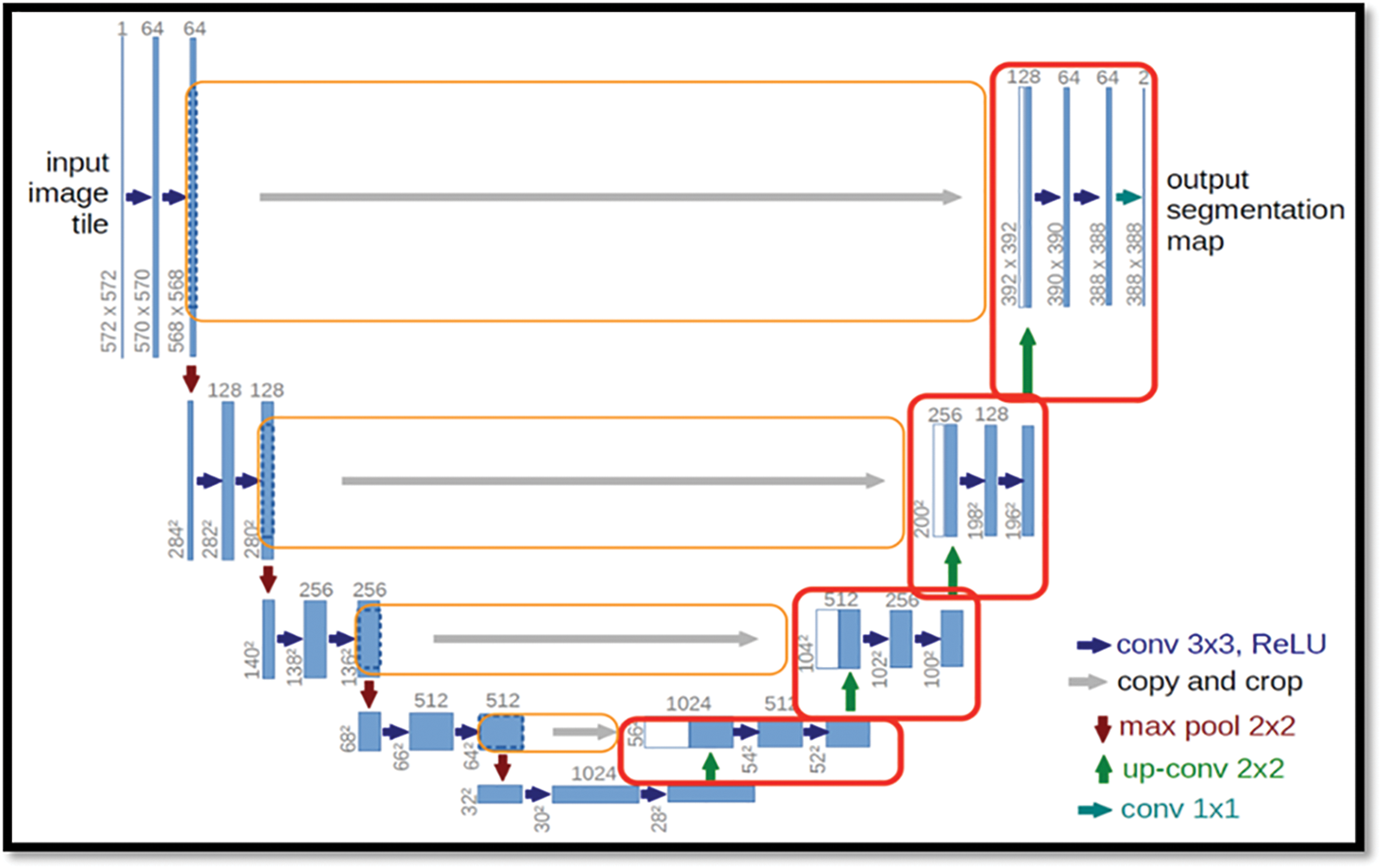
Figure 2: Showing the basic architecture for the Bio-medical images

There is large consent that successful training of deep networks requires many thousand annotated training samples. In this paper, we present a network and training strategy that relies on the strong use of data augmentation to use the available annotated samples more efficiently.

3.1.1 Using the EM Algorithm, the Estimation of Model Parameters

For the current parameter-based logistic type distribution, the likelihood equation is nonlinear and there is no solution by analytic means. Consequently, we use some iterative procedures like the EM algorithm for obtaining the estimates of the parameters.

For Expectation-Maximization (EM) algorithm, the updated equations of the model parameters are

The likelihood of the function of the model is

L(θ)=∏S=1Np(xs,θ(l))(1)

L(θ)=∏s=1N(∑i=1kαifi(xs,θ(l))(2)

This implies

logL(θ)=∑S=1Nlog(∑i=1kαifi(xs,θ(l)))(3)

where θ=(μi,σi2,αi;i=1,2,…k) is the set of initial parameters

Therefore

Three parameter logistic type distribution:-

logL(θ)=∑S=1Nlog[∑i=1mαi[3(3p+π2)][p+(ys−μiσi)2]e−(ys−μiσi)σi[1+e−(ys−μiσi)]2](4)

The process of estimating the likelihood function on sample observations is considered the first step of the EM algorithm and is obtained as,

E-STEP:-

In the expectation (E) step, the expectation value of log L(θ) concerning the initial parameter vector θ(0) is

Q(θ,θ(0))=Eθ(0)[logL(θ)/x¯](5)

Given the initial parameters θ(0). One can compute the density of pixel intensity X as

P(xs,θ(l))=∑i=1kαifi(xs,θ(l))

L(θ)=∏S=1Np(xs,θ(l))

This implies

logL(θ)=∑S=1Nlog(∑i=1kα(l)ifi(ys,θ(l)))(6)

The provisional likelihood which goes to region ‘k’ is

Pk(ys,θ(l))=[αk(l)fk(ys,θ(l))pi(ys,θ(l))]

pk(y,θ(l))=[αk(l)fk(ys,θ(l))∑i=1kαi(l)fi(ys,θ(l))]

For the samples, the log-likelihood function is

Q(θ,θ(l))=Eθ(l)[logL(θ)/y¯](7)

Therefore

For Three parameter logistic type distribution:-

fi(ys,θ(l))=[3(3p+π2)][p+(ys−μi(l)σ(l))2]e−(ys−μi(l)σi(l))σi(l)[1+e−(ys−μi(l)σi(l))]2(8)

M-STEP:-

To get the model parameters estimation, one should increase Q(θ,θ(l)) such that ∑αi=1. This estimation could be achieved by using the first order Lagrange type function

F=[E(logL(θ(l)))+β(1−∑i=1kαi(l))](9)

where β is the Lagrangian multiplier which combines both the log-likelihood functions which need to be maximized. The two steps mentioned above are repeated based on the necessity in which every iteration is used to increase the log-likelihood of the model and the model is used to converge with a likelihood function.

The Updated equations of αi:

To find the expression for αi, we solve the following equation

∂F∂αi=0

∑i=1N1αiPi(ys,θ(l))+β=0

After adding on both sides, β=−N

Therefore,αi=1N∑s=1NPi(ys,θ(l))(10)

The updated equations of αi for (l+1)th iteration is

αi(l+1)=1N∑s=1NPi(ys,θ(l))

This implies

αl(l+1)=1N∑s=1N[αl(l)fl(ys,θ(l))∑i=1kαi(l)fi(ys,θ(l))](11)

The Updated equations of μi:

For updating the parameter μi,i=1,2,3,…k we consider the derivatives of Q(θ,θ(l)) with respect to μi and equal to zero

We have Q(θ,θ(l))=E[logL(θ,θ(l))]

There fore ∂∂μi(Q(θ,θ(l)))=0

Implies E[∂∂μi(logL(θ,θ(l)))]=0

For Two parameter logistic type distribution:-

By applying the derivative with respect to μi, we have

∂∂μi[∑s=1N∑i=1KPi(ys.,θl)logαi[312+π2][4+(ys−μiσi)2]e−(ys−μiσi)σi[1+e−(ys−μiσi)2]]=0(12)

Since μi appears in only one region, i = 1, 2, 3, …k (regions),

For Three parameter logistic type distribution:-

μi(l+1)=∑s=1nPi(ys.,θ(l))(2ys)(σi2)(l)[p+(ys−μi(l)σi(l))2]−∑s=1nPi(ys.,θ(l))σi(l)+∑s=1n2Pi(ys.,θ(l))σi(l)[1+e(ys−μi(l)σi(l))]2∑s=1nPi(ys.,θ(l))(σi2)(l)[p+(ys−μi(l)σi(l))2](13)

The Updated Equation of σi2:

For updating σi2 we differentiate Q(θ,θ(l)),

That is ∂∂σ2(Q(θ,θ(l)))=0

This impliesE[∂∂σ2(logL(θ,θ(l)))]=0(14)

∂∂σi2[∑s=1N∑i=1KPi(ys.,θl)logαi[312+π2][4+(ys−μiσi)2]e−(ys−μiσi)σi[1+e−(ys−μiσi)2]]=0(15)

After simplification the above equation can written as

σi2=∑s=1N[[(ys−μi)σi3]−[1σi2]−[(ys−μi)2σi4(1+e(ys−μiσi)2)]]pi(ys,θ(l))∑s=1N(ys−μi)pi(ys,θ(l))σi4(4σi2+(ys−μi)2)(16)

For Three parameter logistic type distribution:-

∂∂σi2[∑s=1N∑i=1KPi(ys.,θl)logαi[33p+π2][p+(ys−μiσi)2]e−(ys−μiσi)σi[1+e−(ys−μiσi)]2]=0(17)

3.1.2 Initialization of the Parameters by K-Means

Some of the parameters like αi, μ and σi2 are typically measured as identified apriori. A normally cast-off technique in preparing limits is through selecting a arbitrary example from the whole image. If the sample size is small, this method works very well, but it fails when the size of the image is big and some of the regions on the images are not identified fully. In order to solve this problem, the K-means algorithm is used such that to break the images in to homogeneous regions. The procedure for the K-means algorithm is as follows,

Select K data points from the dataset as early clusters randomly and these data points considered as centroids in the initial cases.

By calculating the Euclidean distance from each cluster to the center of the cluster with data points.

Based on the distance value minimum, find the new cluster.

Replication of step 2 and 3 until clustering centers do not change.

End the model implementation.

3.1.3 Segmentation Algorithm

Once the refinement of image parameters process had completed, the important task to be performed in the process of segmentation is the assignment of pixels to the various parts or segments of the image. The process followed in this algorithm is as follows,

Step 1) At first step the histogram of the whole image was plotted.

Step 2) Get the estimates in the initial phases of the model equations by using the K-means algorithm for various regions of the whole images.

Step 3) Get the modified estimates of the model.

Step 4) Allocate a piece pixel to conforming jth region based on maximum likelihood of the model.

Lj=MAX[[3(3p+π2)][p+(ys−μiσi)2]e−(ys−μiσi)σi[1+e−(ys−μiσi)]2],−∞<μi<∞,−∞<σi2<∞,p≥4(18)

3.1.4 Lung Lobe Separation

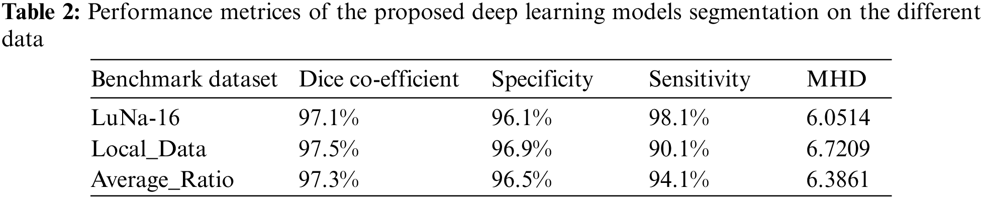
Obtained Initial lung field still contains the main trachea and bronchi. To remove it from the result the 3-D connected component labelling is applied. It removes the trachea and bronchi when they are not connected to the lung region if it is connected then the component labelling will treat it as a part of the lung region and fails to separate it. If trachea and bronchi remain in the results of the component labeling, then 2-D region growing is employed to remove this particular region was clearly visible in the Table 2.

3.2 Image Dataset Description and Data Augmentation

There are thoracic CT scans in the Lung Image Database Consortium image collection (LIDC-IDRI) [16] that have been annotated with lesions for the diagnosis and screening of lung cancer that may be used for diagnostic and screening purposes. Each CT image was reviewed by a radiology specialist who categorized the lesions as “nodule > or = 3 mm,” “nodule 3 mm,” or “non-nodule > or = 3 mm.” Each radiologist reviewed their own markings, as well as the marks of the other three radiologists, before reaching a final judgement during the unblinded-read part of the procedure. Radiologists may do this procedure in one of five ways, they are 1) Highly unlikely for cancer, 2) Moderately unlikely for cancer, 3) Indeterminate likelihood, 4) Moderately suspicious for cancer, 5) Highly suspicious for cancer. The first two categories are identified as benign. The latter two categories were identified as malignant. As a total, 9109 nodular images are obtained.

This was done in order to ensure that the number of better images for each of the three illness groups was shown on the Fig. 3, equal for all three disease groups. As a consequence, there were twice as many images included in the final version as there were in the initial version. With a Gaussian filter with a standard deviation of three pixels, the images were enhanced, as was the edges with a convolutional edge enhancement filter that had a central weight of 5.4 and an 8-surrounding weight of 0.55 and improved the edges’ appearance.

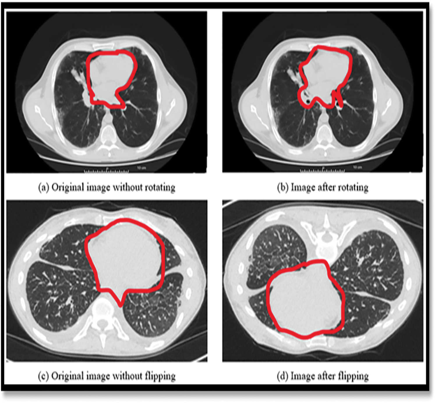
Figure 3: Showing the data augmentation on LuNa-16 dataset images before and after segmentation

3.3 Network Model Architecture

The automatic lung segmentation approach is seen in Fig. 4. In this stage, four critical processes are carried out: trachea and bronchus removal; optimum thresholding; connected component labelling; as well as separation of the left and right lungs. The procedure is detailed in the next section.

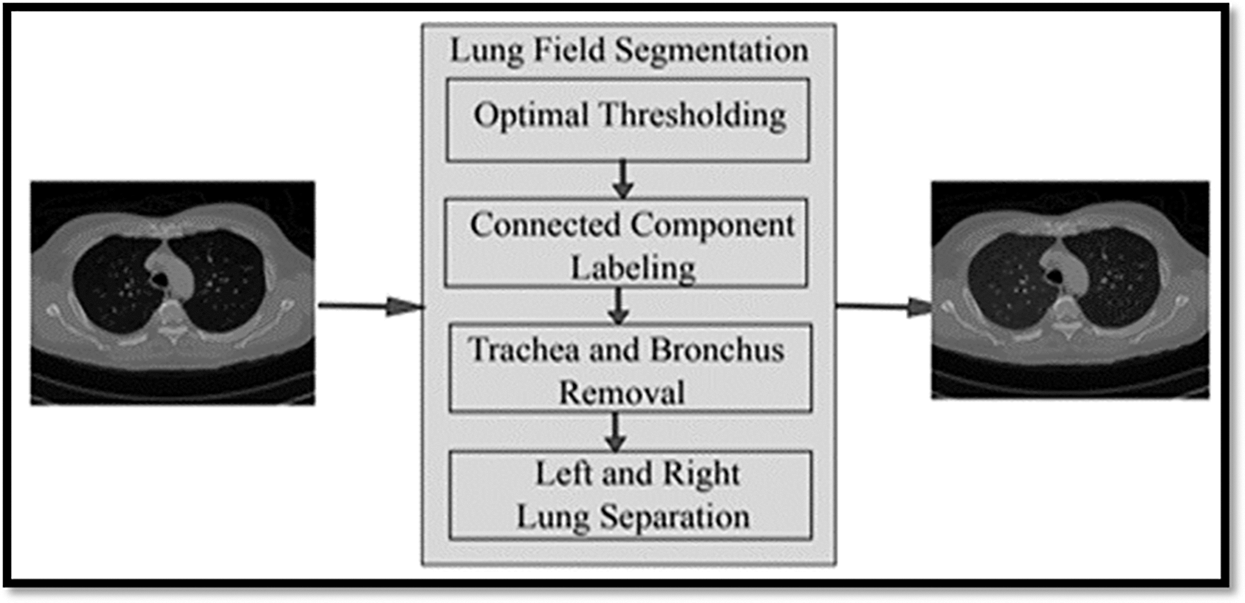
Figure 4: Showing the block diagram of the proposed model

The lung parenchyma, trachea, and bronchial tree are all visible on the first CT scan of the lung. Fat, muscle, and bones may be seen on the exterior of the lung’s anatomy. There are also nodules on the exterior of the lungs, which are called pulmonary nodules.

In order to remove non-parenchymal tissues from a CT image, lung field segmentation must be performed. It is divided into many phases, which are as follows: The trachea and bronchi are removed by the use of a method known as region-growing. This is accomplished when the lung parenchyma has been separated from the surrounding architecture. After the left and right lungs have been put together, there are still certain pieces that need to be removed from the body.

This technique is referred to as “optimal thresholding” (body-voxels). As seen in Fig. 4, lung CT imaging reveals zones of low and high density. There are no voxels that are not part of the body in this image. All of the other voxels in the image are part of the body. When the final run is completed, it displays the precise position of body and non-body voxels.

Suppose that the threshold value is T at step t, which is what we’ll state in the next paragraph. Initially, this threshold was utilized to distinguish between non-body and body voxels in the scene. And the model of the proposed architecture was shown in the Fig. 5.

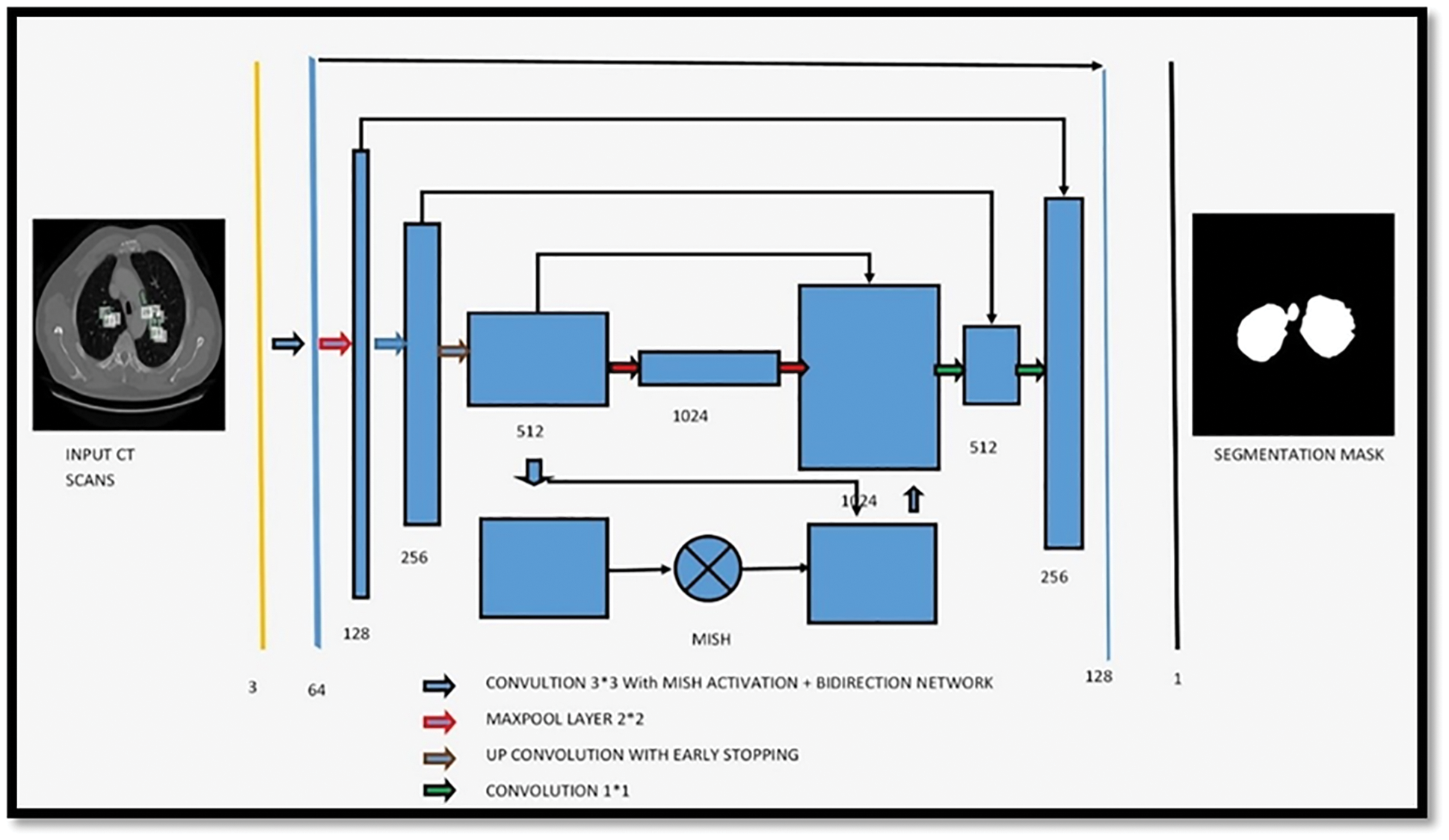
Figure 5: Showing the proposed architecture for segmentation of bio-medical images

3.4 Loss Function of Proposed Network Model

The loss function is as follows:

C(w,b)=12n∑x||y(x)−||2+12nλ∑wW2(19)

where C, w, b, n, x, and an are the cost functions was shown in the Eq. (19). It is used to do the back propagation process, which lowers the discrepancy between anticipated and actual values, hence increasing the accuracy of the process. The U-NET is used to perform the back propagation process. It is critical not to overtrain during the training phase, which is why the last item of the loss function divides the sum of all weights by 2n, which is equal to 2. Another method of preventing overfitting is to drop out. Some neurons are randomly hidden before back propagation, and the parameters are not changed as a result of the masked neurons. In order for the DNN to handle a large amount of data, it also requires a large amount of memory. This is due to the fact that the DNN requires a large amount of data. As a result, when a min batch is executed, a back propagation is carried out in order to allow for more rapid parameter changes. The activation function of the neural network is known as Leaky ReLU, and it is responsible for helping it simulate objects that are not straight lines. The activation function of the ReLU is represented by the following mathematical formula of the Eq. (20).

y={xoifx>0;x<0(20)

In the example below, x represents the outcome of priority-weighted multiplication and paranoid addition, while y represents the output of an activation function, as indicated in the Fig. 6 above. If x is less than zero, the answer is zero; if x is more than zero, the answer is one. Therefore, ReLU is capable of resolving the issue of the sigmoid activation function’s gradient. Weights cannot be modified indefinitely, however, since training is always being updated, which is referred to as “neuronal death” in the scientific community. The output of ReLU, on the other hand, is larger than zero, indicating that the output of the neural network has been modified. The usage of leaky ReLUs might be utilized to overcome the concerns described above. The activation function for the Leaky ReLU is represented by the following formula Eq. (21).

y={xoifx>0;x<0(21)

where a is set to 0.1; a in Leaky ReLU is fixed and in the ReLU is not fixed.

Figure 6: Showing the loss function of the proposed classifier

3.5 Activation Function

An activation function is used by a Neural Network to take use of the concept of non-linearity. ReLU, TanH (Tan Hyperbolic), Sigmoid, Leaky ReLU, and Swish are examples of such algorithms. This work introduces a novel activation function, denoted by the letters Mish. Mish may be calculated using the formula f(x) = softplus(x) tanh. Classification performance was shown on the Fig. 7i. Because Mish and Swish are so similar, it is simple for researchers and developers to include Mish into their Neural Network Models. Mish also performs better and is simpler to set together than other options.

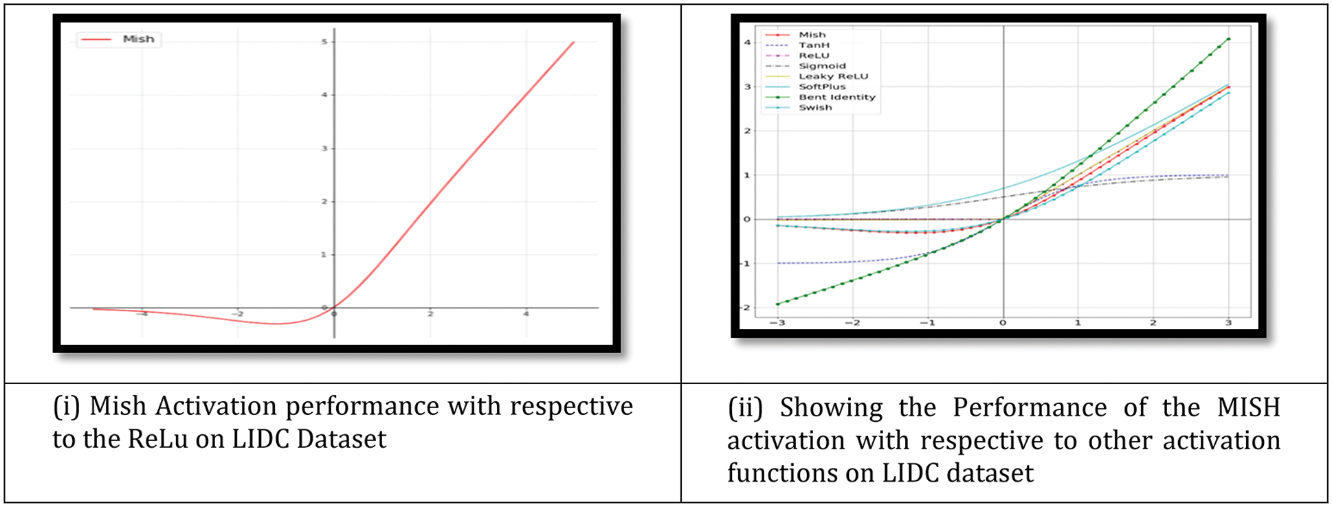
Figure 7: (i) Showing the graph of Mish activation function (ii) Showing the Mish activation with respective to other activation function. Mish outperformed when compared with other functions on the LIDC dataset

Mish’s characteristics, such as being unbounded above and below, smooth, and nonmonotonic, all contribute to his superior performance when compared to other activation functions. As a result of the wide variety of training conditions available, it is difficult to determine why one activation function performs better than another. Fig. 7ii depicts a large number of activation functions. The graphs of Mish activation are shown next to them. For example, as seen in Fig. 8, owing of Mish’s non-monotonic property, tiny negative inputs are maintained as negative outputs, which improves the expression and gradient flow. Due to the fact that the order of continuity of Mish is infinite, it has a significant advantage over ReLU, which has an order of continuity of 0. Due to this, ReLU cannot be continuously differentiable, which may make gradient-based optimization more challenging for those that employ it.

Figure 8: Showing the sharp transition between the ReLU and MISH

Due to the fact that Mish is a smooth function, it is easy to optimize and generalize, which is why the results became better with time. To determine how well ReLU, Swish, and Mish performed, the output landscape of a five-layer, randomly-initialized neural network was examined for each of them. We can see how rapidly the scalar magnitudes for ReLU coordinates shift from Swish and Mish to the current Fig. 8 Because of this, a network that is simpler to regulate has smoother transitions, which in turn results in loss functions that are smoother. This makes it simpler to generalize the network, which is why Mish performs better than ReLU in several domains compared to ReLU. The landscapes of Mish and Swish, on the other hand, are very similar in this regard.

4  Results and Discussions

Additionally, complementary labelling is used in U-Net training. Two-dimensional data should be treated similarly to one-dimensional data. The model seeks to eliminate as many labelling mistakes as feasible in both directions. By comparison, the mass of each pixel decreases with time. Engaging with them accomplishes the two-fold objective.

In Table 3, we compare the results of numerous approaches on our test data with and without pre-processing (with CLAHE, wiener filter, and ROI segmentation). The sensitivity improves from 91.65% to 96.5% after pre-processing, and the dice coefficient increases from 94.56% to 97.3%. This study examines a variety of labeling strategies, both monolithic and hybrid. The term “mono” refers to a single label input, while “hybrid” refers to a single label input with either a positive or negative output (complementary labeling) (complementary labeling). Regardless matter whether the model is trained on positive or negative ground truth, the output can never be better than the mono input. Complementary labeling seems to be ineffective when dealing with large data sets.

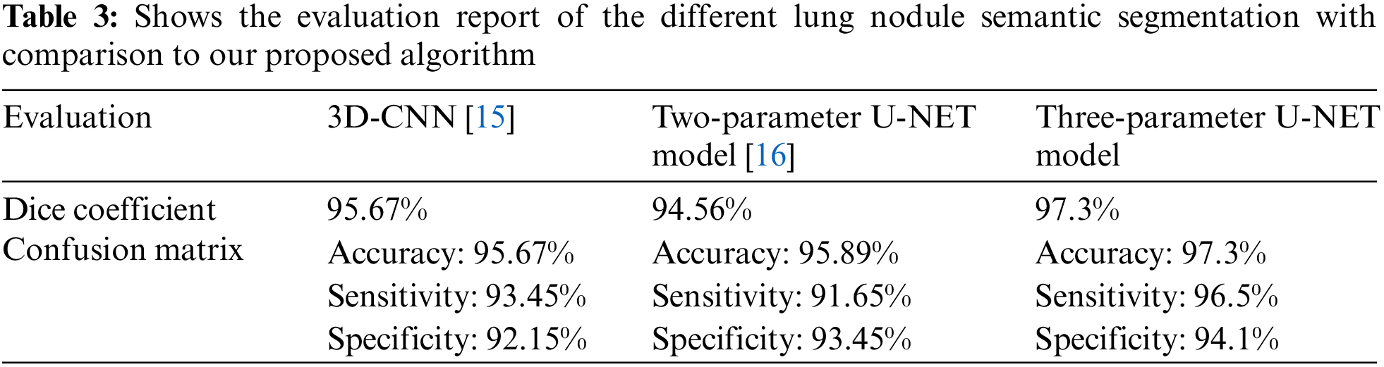
This research examines data from a variety of sources and includes 472 and 50 occurrences, respectively. Complementary labeling and pre-processing, as demonstrated in Tables 4–6, outperform mono input in the majority of cases. On the other hand, complementary labeling is ineffective in the absence of pre-processing. When dealing with little amounts of data, complementary labeling may be quite beneficial. As a result, this research examines the viability of labeling enhancement. Hybrid negatives are preferred over mono-input positives because smaller data volumes are more sensitive to hybrid negatives. Positive mono outputs provide a value of 90%, whereas negative hybrid inputs produce a value of 92% and the output of the results can be seen in Fig. 9. If the data set is insufficient, more labels may be necessary to round.

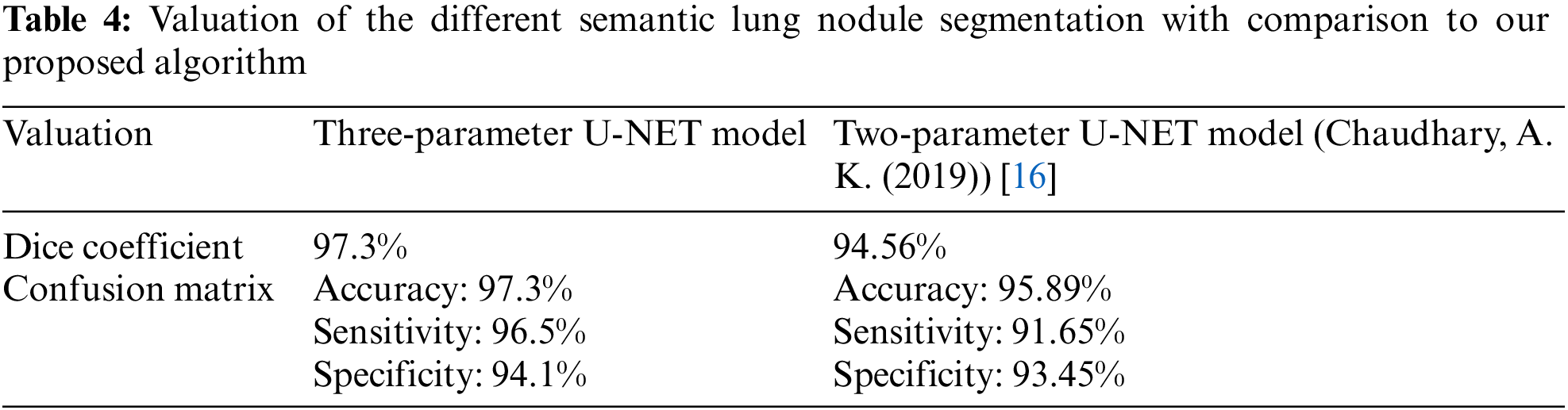
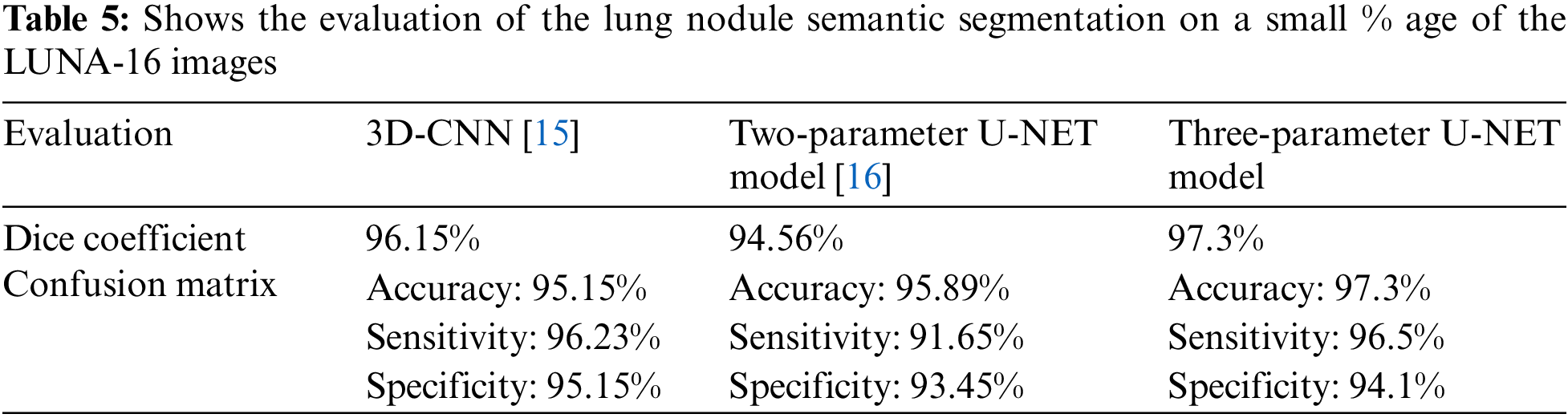
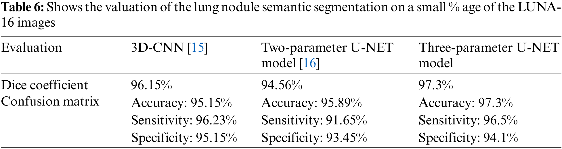
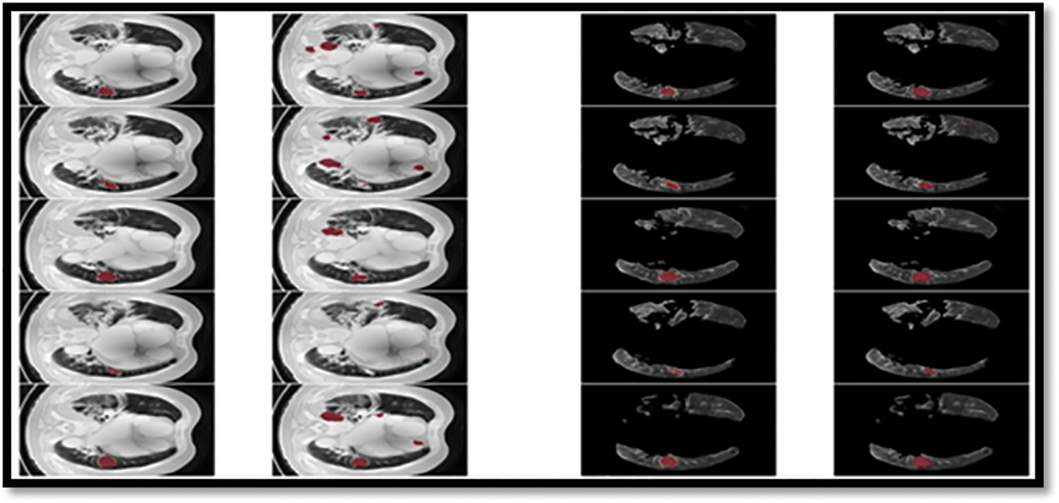
Figure 9: The ground truth prediction before segmentation and after segmentation

The U-NET algorithm for the lung tumor segmentation model has been implemented in TensorFlow and tested its efficiency for image segmentation. The LUNA-16 images are considered for image segmentation. The performance of both two-parameter and three-parameter logistic type distributions follows. The pixel intensities of the image are assumed to follow a mixture of two-parameter logistic type distribution and three parameter logistic distribution was shown in the Tables 7 and 8.

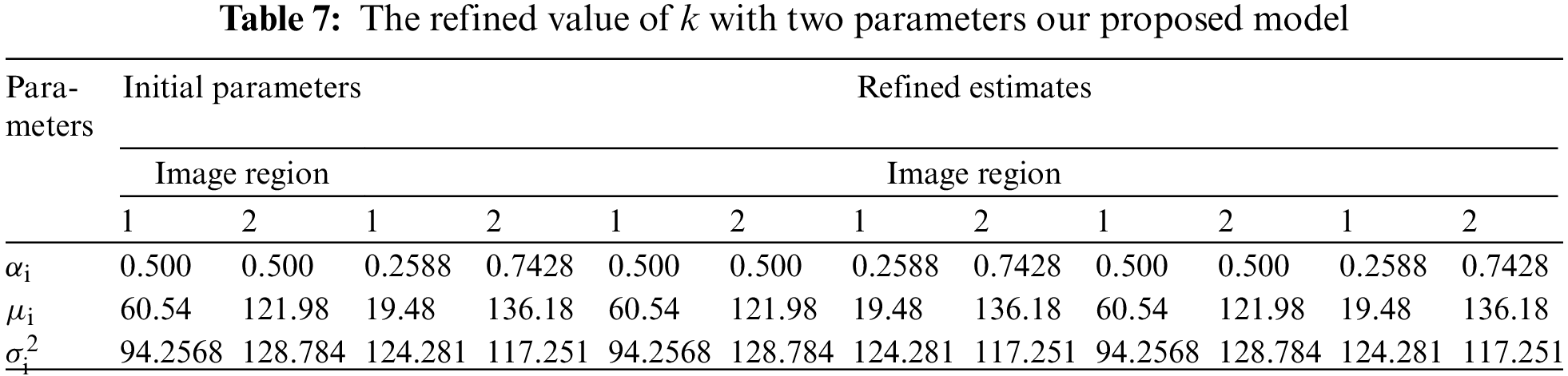
We consider that the image contains k regions and pixel intensities in each image region follow a two-parameter logistic type distribution with different parameters. The number of segments in each of the CT scans images considered for experimentation is determined by the histogram of pixel intensities. The histograms of the pixel intensities of the CT scan images.

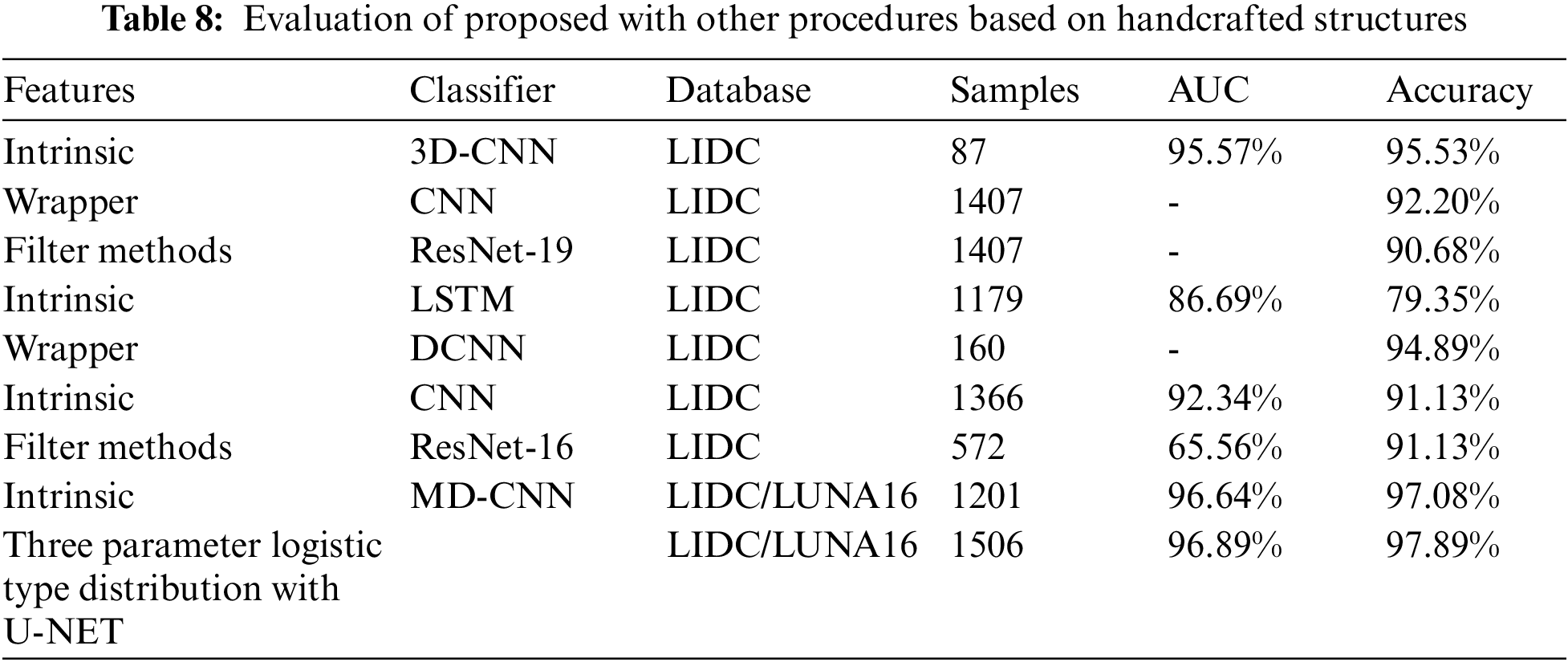
From the Table 8. it was very clear that our classifier U-Net with three parameters logistic has outperformed remaining all the classifiers in terms of the performance metrics like AUC and accuracy on LUNA 16 benchmark dataset.

From the Table 8, it was clearly evident that our method was performed very well with few samples size from LUNA 16 dataset. The results clearly shows that out proposed model and method are good at classifying odd benign and Malignant tumours. As, a result the model has achieved a trust gain when compared with various others methods and clear output was shown in Fig. 10.

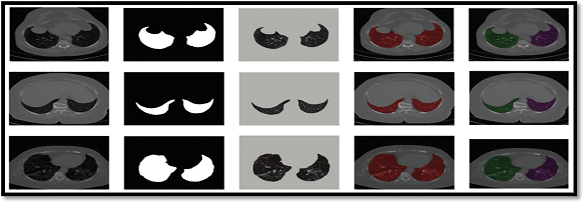
Figure 10: Showing the proposed classifier on LuNa-16 dataset. Second column showing the original image, third column showing the Lung Lode, and last two is the segmented image

5  Conclusion

For the purposes of this research, we used improvised U-NET and limited EM with Logistic type distribution for the (U-NET with three parameters logistic distribution) to make it simple to distinguish between various portions of the lung. It makes use of the spatial interaction of neighboring voxels to create images that are visually distinct. Semantically segmenting CT scans of lung cancer patients is important because it will help find the disease and figure out how worsened the tissue. This will make it easier to figure out which patients need treatment first. We have proposed a Computer Aided Diagnosis (CAD) systems ways to find infected lung tissue in CT scans. Having this kind of technology available during the current pandemic will make it easier to automate, prioritize, speed up, and expand treatment for patient care around the world.

6  Future Work

The assessment performed in this research enables further development of the concepts identified in this study, which may be used to the construction of a high-accuracy CAD system. Based on this research, it is possible that future research will go the following routes.

•   In order to increase the accuracy and robustness of this tool’s classification of all other forms of lung nodules in the future, we will seek to improve its accuracy and robustness for all other types of nodules.

•   To determine if the suggested approach can be utilized as a therapy, it will be evaluated on a variety of datasets in the near future.

•   In the future, it will be able to classify nodules according to their characteristics. This will be included into the framework for segmenting lung nodules.

Funding Statement: This research was financially supported by the Ministry of SMEs and Startups (MSS), Korea, under the “Startup growth technology development program (R&D, S3125114)” and by the Ministry of Small and Medium-sized Enterprises (SMEs) and Startups (MSS), Korea, under the “Regional Specialized Industry Development Plus Program (R&D, S3246057)” supervised by the Korea Institute for Advancement of Technology (KIAT).

Conflicts of Interest: The authors declare that they have no conflicts of interest to report regarding the present study.

References

1. World Health Organization (WHO“Cancer,” 2022. [Online]. Available: https://www.who.int/en/newsroom/fact-sheets/detail/lungcancer. [Google Scholar]
2. N. Zhang, J. Lin, B. Hui, B. Qiao, W. Yang et al., “Lung nodule segmentation and recognition algorithm based on multiposition U-net,” Computational and Mathematical Methods in Medicine, Vol. 2022, pp. 11, 2022. [Google Scholar]
3. Y. Jalali, M. Fateh, M. Rezvani, V. Abolghasemi and M. H. Anisi, “ResBCDU-Net: A deep learning framework for lung CT image segmentation,” Sensors, vol. 21, no. 1, pp. 268, 2021. [Google Scholar]
4. M. Kumar, V. Kumar and A. Sharma, “Segmentation and prediction of lung cancer CT scans through nodules using ensemble deep learning approach,” in IEEE Mysore Sub Section Int. Conf. (MysuruCon), Hassan, India, 2021, pp. 781–785, 2021. [Google Scholar]
5. K. Shankar, E. Perumal, V. GarcíaDíaz, P. Tiwari, D. Gupta et al., “An optimal cascaded recurrent neural network for intelligent COVID-19 detection using chest X-ray images,” Applied Soft Computing, vol. 113, no. 3, pp. 107878, 2021. [Google Scholar]
6. Y. Cui, H. Arimura, R. Nakano, T. Yoshitaka, Y. Shioyama et al., “Automated approach for segmenting gross tumor volumes for lung cancer stereotactic body radiation therapy using CT-based dense V-networks,” Journal of Radiation Research, vol. 62, no. 2, pp. 346–355, 2021. [Google Scholar]
7. A. G. Sauer, R. L. Siegel, A. Jemal and S. A. Fedewa, “Current prevalence of major cancer risk factors and screening test use in the United States: Disparities by education and race/ethnicity,” Cancer Epidemiology and Prevention Biomarkers, vol. 28, no. 4, pp. 629–642, 2019. [Google Scholar]
8. M. Polsinelli, L. Cinque and G. Placidi, “A light CNN for detecting COVID-19 from CT scans of the chest,” Pattern Recognition Letters, vol. 140, no. 6, pp. 95–100, 2020. [Google Scholar]
9. M. Naseriparsa and M. M. R. Kashani, “Combination of PCA with SMOTE resampling to boost the prediction rate in lung cancer dataset,” International Journal of Computer Applications, vol. 77, no. 3, pp. 33–38, 2013. [Google Scholar]
10. I. Ibrahim and A. Abdulazeez, “The role of machine learning algorithms for diagnosing diseases,” Journal of Application Science and Technology Trends, vol. 2, no. 1, pp. 10–19, 2021. [Google Scholar]
11. F. Farheen, M. Shamil, N. Ibtehaz and M. S. Rahman, “Revisiting segmentation of lung tumors from CT images,” Computers in Biology and Medicine, vol. 144, pp. 144–148, 2022. [Google Scholar]
12. Y. C. Chang, Y. C. Hsing, Y. W. Chiu, C. C. Shih, C. Lin et al., “Deep multi-objective learning from low-dose CT for automatic lung-rads report generation,” Journal of Personalized Medicine, vol. 12, no. 3, pp. 417–421, 2022. [Google Scholar]
13. H. Yu, J. Li, L. Zhang, Y. Cao, X. Yu et al., “Design of lung nodules segmentation and recognition algorithm based on deep learning,” BMC Bioinformatics, vol. 22, no. 314, pp. 263–281, 2021. [Google Scholar]
14. S. Kido, S. Kidera, Y. Hirano, S. Mabu, T. Kamiya et al., “Segmentation of lung nodules on CT images using a nested three-dimensional fully connected convolutional network,” Frontiers in Artificial Intelligence, vol. 5, no. 3, pp. 1–9, 2022. [Google Scholar]
15. S. N. J. Eali, D. Bhattacharyya, T. R. Nakka and S. P. Hong, “A novel approach in bio-medical image segmentation for analyzing brain cancer images with U-NET semantic segmentation and TPLD models using SVM,” Traitement du Signal, vol. 39, no. 2,. pp. 419–430, 2022. [Google Scholar]
16. D. Bhattacharyya, N. M. J. Kumari, E. S. N. Joshua and N. T. Rao, “Advanced empirical studies on group governance of the novel corona virus, mers, sars and ebola: A systematic study,” International Journal of Current Research and Review, vol. 12, no. 18, pp. 35–41, 2020. [Google Scholar]
Cite This Article
Copyright © 2023 The Author(s). Published by Tech Science Press.
This work is licensed under a Creative Commons Attribution 4.0 International License , which permits unrestricted use, distribution, and reproduction in any medium, provided the original work is properly cited.
Downloads
Citation Tools