Modeling and TOPSIS-GRA Algorithm for Autonomous Driving Decision-Making Under 5G-V2X Infrastructure

1  Introduction

In recent years, the transport industry integrated with 5G telecommunication technology has prompted the development of the intelligent connected vehicles (ICVs) industry. The channel bandwidth of the 5G-V2X (vehicle-to-everything) wireless network is approximately 400 MHz, transmission latency is less than 1 ms, and positioning accuracy is below 0.1 m; which is 20, 10, and 100 times higher than those indexes of LTE-V2X network, respectively [1,2]. Meanwhile, the transmission reliability of the 5G-V2X network has reached 99.999%, also far above that of the LTE-V2X network. By incorporating vehicles into a connected automated transport system, 5G-V2X technology makes it possible to control ICV autonomous driving in a real-time manner by employing cloud computing and big data of traffic scenarios [3,4].

Under 5G-V2X road infrastructure, ICV’s environmental perception system is enhanced by fusing vehicle-to-vehicle (V2V), vehicle-to-infrastructure (V2I), vehicle-to-pedestrian (V2P), and vehicle-to-network (V2N) with on-board environmental perception system. These facilities or instruments contain GPS/INS (global positioning system and inertial navigation system), 3-dimensional LiDAR, multichannel radar, high-resolution cameras, wheel speed sensors, etc. In 2016, the society of automotive engineers (SAE) defined 6 levels of autonomous driving and levels 3 to 5 of which were classified as advanced autonomous driving [5]. In 2020, China released the ICVs Technology Roadmap 2.0, in which levels 4 and 5 were defined as vehicles, roads, and pedestrians connected to cooperative control of self-driving in urban areas.

The ultimate objective of autonomous driving is to realize human-like driving behavior [6,7]. In the vehicle moving process, the driver’s task is to perceive the road environment, predict the intention of moving obstacles, determine driving behavior, and control vehicle direction and velocity to reach the expected goal [8]. Generally, drivers take pedestrians, vehicles, and the road as an integrated system, and perform actions in a reactive-driving way [9,10] inspired by scene understanding, a priori knowledge, and driving intention. Through human sense organs, mainly eyes, ears as well as noses, drivers previously collect real-time information about traffic flow, ego-vehicle state, and traffic signals; transmitting this multi-source information to the cerebrum system for further processing. By mining this information, the cerebrum gets key information about ego-vehicle movement; sequentially, the cerebrum infers an optimal driving behavior by comparing it with the prior trained driving models as well as traffic rules [11]. When designing a decision-making model for ICV autonomous driving, we should learn from the process of experienced drivers dealing with different traffic scenarios, and pursue a cerebrum-like decision-making method.

ICV autonomous driving system can be separated into 5 logic modules: global path planning, driving behavior decision-making, local movement path planning, vehicle operation control system, and implementation instrument, as shown in Fig. 1. Under 5G-V2X smart road infrastructure, when ICV starts autonomous driving, the global path planning module firstly utilizes GPS/INS positioning information and road network document (RND) to search vehicle position code, current road code or field driving code. Subsequently, by including a mission document (MD), this module plans a task and a series of implementable actions for traveling along this special road or field [12]. In this article, we focus on developing a cerebrum-like decision-making model for ICV self-driving system design.

Figure 1: Framework of ICV cerebrum-like autonomous driving system under 5G-V2X infrastructure

Fig. 1 reveals that the driving decision-making module extracts relative information from the real-time raster map, herein, it classifies this information as a discrete event set that delineates current traffic scenario understanding, global path output, traffic rules, a priori knowledge of the experienced driver, and intention of dynamic obstacles, etc. In the following steps, this module further divides ICV routine driving actions into different driving behavior states and infers a reasonable real-time driving behavior based on the above discrete event set [13,14]. This module transforms the inference results into a goal point set, and sends it to the local movement path planning module, meanwhile producing feedback to the global path planning module to update global information simultaneously. According to the position of goal points, through probing current traffic scenario information, driving priori knowledge, ego-vehicle dynamic characteristics, as well as vehicle kinematics/dynamics constraints, the local movement path planning module plans an optimal local path-point sequence and an expected velocity [15]. Similarly, this module sends movement planning results to the vehicle control system, at the same time pulsating feedback to the decision-making module to update input data in a real-time manner. Restricted by ego-vehicle position and kinematics/dynamics model, through mining data of local path-point sequence, expected velocity, driving scenario information, and priori knowledge, the operation control module generates data of velocity, acceleration, steering angle, and yaw rate; subsequently, it sends this data to vehicle implementation facilities. Also, this module still pulses feedback to the upper module to refresh local path planning data. In the end, the vehicle implementation module produces a series of implementable orders, including throttle opening degree, brake pedal switch and steering wheel angle, etc., to drive the vehicle in a safe, efficient and comfortable manner. Simultaneously, it sends feedback to the control module to update real-time controller data.

Developed by Stanford University, the Junior autonomous vehicle adopted a finite state machine (FSM) model to make driving behavior decisions [16,17]. Its state set contains 14 driving behaviors, i.e., initial state, driving forward, lane following, collision avoidance, waiting at a stop sign, driving through intersections, waiting at an intersection, U-Turn, stopping at a U-Turn, crossing a yellow line, driving in parking lots, driving on traffic congestion road, driving on mismatched RND road, and mission termination. These behaviors include almost all driving states that Junior autonomous vehicles would encounter when driving in an urban road environment. The Junior decision-making system is functionally based on FSM’s behavior state set and event set [18,19]. Besides the FSM model, other models such as the Prolog inference engine, Markov decision process, Bayesian decision tree, swarm intelligence, etc., are also applied to autonomous driving decision-making [20,21].

The FSM model is a rule-based discrete input/output control system that supports dynamic model construction [22]. Since the FSM model has characteristics of time-varying and nonlinear transition, it is extensively used for robotic model construction. The FSM model has finite states, the current state receives events and then infers corresponding actions to motivate a change to the current state [23]. The FSM model is composed of 4 components: event set, state set, transition, and action [24]. The event set describes the input conditions that trigger state transformation and is defined as a series of input quantitative or qualitative information. State set depicts forms of the object and is determined by event data, implementing special action, or waiting for a specified event. Transition delineates possible paths among each state, which means that the FSM model will transit from the current state to another state when emerging specified events or implementing special actions. Action is a state indicating the FSM’s decision-making result, and is also the initial state of the next time point. It is carried out through lower layer modules, i.e., local movement planning module, vehicle operation control module, and implementation module. The FSM model may take matrices or state transformation tables to display data or information. When constructing an FSM model, one needs to clearly define elements as well as their characteristics in each set according to the designed object [25].

This paper is to explore the cerebrum-like decision-making problems for ICV advanced autonomous driving under 5G-V2X road infrastructure. Compared with the existing literature, the main contribution is that this paper proposes a hierarchical finite state machine (HFSM) as well as a TOPSIS-GRA algorithm that can perform cerebrum-like decision-making behavior for ICV autonomous driving. PreScan simulative experiments have shown that the proposed HFSM model and TOPSIS-GRA algorithm can meet the requirements of ICV autonomous driving decision-making under 5G-V2X infrastructure. The following work is organized as: Section 2 builds a mealy HFSM model for ICV cerebrum-like decision-making based on the traditional mealy FSM model. To realize data fusion in a modeling process, Section 3 develops a TOPSIS-GRA algorithm for state transition of the HFSM model by combing TOPSIS and GRA algorithms together. To verify the proposed cerebrum-like autonomous driving decision-making model, Section 4 firstly constructs a series of traffic scenarios, and thereafter performs simulative experiments on the PreScan8.50 platform. Section 5 explains the experiment results and further conducts a discussion. Finally, a brief conclusion is summarized in Section 6.

2  HFSM Model for Autonomous Driving Decision-Making Under 5G-V2X Infrastructure

Under 5G-V2X intelligent road infrastructure, ICV’s environmental perception system adds newborn external V2V, V2I, V2P, and V2N approaches by installing relative onboard units (OBUs). Fusing with ICV internal installed sensors, such as cameras, 3-dimensional LiDAR, millimeter-wave radar, wheel speed sensor, GPS/INS receiver, etc., ICV may collect all-around information about current traffic scenarios, even outperforming the environmental perception of a human driver. Meanwhile, through utilizing a 5G network to transmit data and a cloud computing platform to assist data processing, ICV has greatly enhanced real-time data processing, therefore, information latency is well decreased. This section constructs an HFSM decision-making model [23] for ICV self-driving under 5G-V2X intelligent road infrastructure. It is comprised of a global driving FSM model and a local driving FSM model. Logically, the output of the former is a partial input of the latter; and the output of the latter acts as a partial input of the next module, simultaneously pulsating feedback to the global FSM model to refresh real-time input signals as well as correcting the decision-making result when mismatched with current traffic scenario.

2.1 Global FSM Model

When constructing an FSM model for ICV autonomous driving decision-making, the signal processor employs discrete change events as the input signals. It is responsible for mining data from the raster map and handling this data to generate quantitative events. These events contain external events and ego-vehicle characteristic events. The former is the current traffic scenario data collected by onboard sensors and V2X receivers; and the latter includes velocity, acceleration, steering angle, and yaw rate, etc., which are monitored by onboard sensors. The driving behavior decision-making module has finite driving states, and each state indicates the special control approach of the ego-vehicle. As shown in Fig. 1, when inputting external and internal events, the driving decision-making module firstly handles this data and thereafter infers a corresponding driving state to respond to the current traffic scenario.

Fig. 2 delineates the state transition graph of the global FSM model. When ICV drives autonomously on a 5G-V2X structured smart road, it simultaneously infers an optimal driving behavior according to the information from environmental perception systems such as a raster map, ego-vehicle’s moving characteristics, and driving priori knowledge, etc. When confronted with different traffic scenarios, ICV self-driving needs to focus on special information collected by different sensors. For example, when driving along a linear lane, it may omit traffic light information; when crossing an intersection, it may neglect lane line detection. For ICV self-driving model construction, recognizing and utilizing the priori knowledge may enhance decision-making efficiency or effectiveness. Based on different traffic scenarios under 5G-V2X intelligent road infrastructure, the global FSM is defined as a triple array F=(S,E,Tr). Where S={S1,…,Sm} is the state set of FSM and Si(i=1,2,…7) indicates the state of start, on road, approaching an intersection, intersection, field driving, U-Turn, and stop, respectively [22]. Tr is a state transition algorithm, in mathematics terms, Tr:S×E→S. And E={e1,…,en} is the FSM’s event set, i.e., causation of driving behavior state. Concretely, each element ej(j=1,…,17) is defined as,

Figure 2: State transition graph of the global FSM model

e1: the ego-vehicle’s current speed, unit: km/h;

e2: the distance belongs to an interval (100, M] between the ego-vehicle’s GPS position and the entrance of the first intersection, and M denotes a positive number far above 100 m. unit: m;

e3: the distance belongs to an interval (0, 100] between the ego-vehicle’s GPS position and the entrance of the first intersection. unit: m;

e4: the distance belongs to an interval (−M, 0] from the ego-vehicle’s GPS position back to the entrance of the first intersection. unit: m;

e5: the distance belongs to an interval (100, M] between the ego-vehicle’s GPS position and the exit of the first intersection. unit: m;

e6: the distance belongs to an interval (0, 100] between the ego-vehicle’s GPS position and the exit of the first intersection. unit: m;

e7: the distance belongs to an interval (−M, 0] from the ego-vehicle’s GPS position back to the exit of the first intersection. unit: m;

e8: next task of the mission document (MD) is field driving and the distance belongs to an interval (100, M] between the ego-vehicle’s GPS position and the next task point. unit: m;

e9: MD’s next task is field driving and the distance belongs to an interval (0, 100] between the ego-vehicle’s GPS position and the next task point. unit: m;

e10: MD’s current task is field driving and the distance belongs to an interval (100, M] between the ego-vehicle’s GPS position and exit of the global path’s last field driving. unit: m;

e11: MD’s current task is field driving and the distance belongs to an interval (0, 100] between the ego-vehicle’s GPS position and exit of the global path’s last field driving. unit: m;

e12: the distance belongs to an interval (0, 100] between the ego-vehicle’s GPS position and the mission terminal point. unit: m;

e13: the distance belongs to an interval (100, M] between the ego-vehicle’s GPS position and the mission terminal point. unit: m;

e14: MD’s next task point is a U-Turn and the distance belongs to an interval (0, 100] between the ego-vehicle’s GPS position and the next task point. unit: m;

e15: the distance belongs to an interval (0, 100] between the ego-vehicle’s GPS position and U-Turn, and the angle of driving direction and next road section is less than 10 degrees. unit: m;

e16: MD’s previous task point is a U-Turn and the distance belongs to an interval (0, 100] between the ego-vehicle’s GPS position and the U-Turn. unit: m;

e17: the distance belongs to an interval (0, 100] between the ego-vehicle’s GPS position and U-Turn, and the angle of driving direction and previous road section is less than 10 degrees. unit: m.

By applying the state transition algorithm in Section 3 to handle the global FSM’s decision-making matrix A0=(a0,ij)7×17, we can get the decision-making result of the global FSM model. As an input signal, the result is transmitted to the local FSM model, simultaneously, the system produces feedback to the upper module to real-time update the global path, as displayed in Fig. 1.

2.2 Local FSM Model

The goal of the driving behavior decision-making module is to generate objective points for the local movement path planning module to plan a feasible, safe, and comfortable local path in a real-time situation. When a human driver drives a vehicle on the road, his/her driving behavior can be classified as a series of driving states. Driving behavior is the driver’s controlling and operating behavior in response to the coupled states of ego-vehicle and the current road environment. In general, the decision-making results of driving behavior contain lane change, lane following, turning movement, obstacle avoidance, vehicle following, stop, etc. [26,27]. To deal with different driving behaviors, this paper designs a local FSM’s state set by considering different traffic scenarios. Concretely, the set has 16 driving states, i.e., {start, lane following, acceleration, deceleration, vehicle following, overtaking vehicles, turn left to avoid obstacles, turn right to avoid obstacles, change to left lane without deceleration, change to right lane without deceleration, change to left lane with deceleration, change to right lane with deceleration, U-Turn, stop at an intersection, stop at roadside, stop at parking lots}. According to evaluations of 10 experienced drivers as well as driving scenarios simulation in the PreScan8.50 environment, the HFSM model state set can meet the requirements of ICV autonomous driving under 5G-V2X intelligent road infrastructure.

As ICV needs to determine candidate goal points for the selected driving state when making an autonomous driving decision, the local FSM model adds a candidate goal points set—in mathematical terms, it is a quaternion array F=(S,E,Tr,V). Where S={x1,…,xm} is the state set in the local FSM and xi sequentially denotes the above 16 driving states. E={f1,…,fn} is the event set in the local FSM and fj is determined according to different states of the global FSM. V={V1,…,Vv} is a set of candidate goal points. And Tr is a state transition algorithm, also Tr:S×E→S.

The state set in the local FSM is comprised of the above 16 driving states. However, how to determine the event set in the local FSM is a little bit uncertain and artificial. Wilde [28] reports that drivers always put their ego-vehicle’s driving state into self-monitoring, continuously evaluate their driving behavior and take the result as the ego-vehicle’s driving risk. Although the concept of driving risk delineates the driver’s understanding of the current traffic scenario, it is yet a qualitative evaluation and hard to be measured quantitatively or accurately. In general, drivers mainly focus on three factors: driving safety, travel efficiency, and ride comfort in the vehicle movement process [29]. Andrievsky et al. [30] and Zu et al. [31] apply a curving line to describe the relationship between driving safety and velocity gradient, and they support that driving safety is enhanced when the velocity gradient is decreased. Jung et al. [17] and Constantinescu et al. [32] construct a risky driving model to monitor driving risk based on detecting the distance between ego-vehicle and peripheral vehicles. This model identifies that driving safety is in a positive proportion to the distance, which implies that the driver’s distance estimation is vital to driving safety. Besides safety concerns, driving efficiency is also a major concern of drivers in the vehicle movement process. In reality, drivers always hope to reach the terminal mission point as fast as possible, and the possible highest speed is called the expected speed [17]. Concerning ride comfort, it is mainly related to factors of acceleration, path curvature, steering angle, and yaw rate. In Fig. 1, it acts as an important index to evaluate the lower layer modules and has little relation to the driving behavior decision-making module. Based on driving safety and travel efficiency indexes in risky driving theory, this paper classifies traffic scenario information as features of the multiple attribute decision-making (MADM) approach [33] and then designs the event set in the local FSM model.

On condition of the global FSM output being {on road}, events of the local FSM can be defined as follows.

f1: the distance between the ego-vehicle and the left roadside is d1=3.5N−3.5(n−1)−1.75, where N is the total lane number of the current road section, and n denotes the order of the current lane.

f2: the distance between the ego-vehicle and the right roadside is d2=3.5(n−1)+1.75.

f3: the distance between the ego-vehicle and obstacles on the left lane, which is measured as d3=min{d(egovehilce,obstaclei)|i=1,…,I}.

f4: the distance between the ego-vehicle and obstacles on the right lane, and d4 has a similar formula to d3, the only difference among which is the lane located on the ego-vehicle’s right hand.

f5: security index of ego-vehicle in the current lane. ISO [34] provides a formula to test secure distance at different speed levels. It needs to consider two factors: the distance between the ego-vehicle and the immediate forward vehicle, and the time delay of the ego-vehicle’s implementation facility (the amount of time of driving decision-making, the results transmission, local movement path planning, local path results transmission, and implementation facility response). Collision avoidance measurement is based on the fact: assuming the distance between the ego-vehicle and the forward vehicle is Ds, if the forward vehicle suddenly implements a brake action, collision will not occur on condition that the ego-vehicle’s moving distance from deceleration to stop is less than Ds plus forward vehicle moving distance. Therefore, the security index can be measured as D=vseft2/(2aseft)+vseft∗t−vforward2/(2aforward); and m=(Ds−D)/Ds if Ds>D, otherwise m=ε. Where t denotes the time delay of the ego-vehicle’s implementation facility, a is average acceleration, D indicates the warning distance, and m is the security index. Obviously, the bigger m means the lower risk of collision.

f6: time of ego-vehicle getting the previewed goal point, which is calculated as T=d(self,goal)/vself. According to preview-follower theory [35] and the experiences of skilled drivers, this paper sets the distance between the ego-vehicle and previewed goal point as, (i) 500 m if driving on a line lane, (ii) the length from the ego-vehicle to the tangent point determined by the ego-vehicle and forward roadside curve if driving on a bend lane or intersection, or (iii) the length from ego-vehicle position to the nearest forward obstacle.

f7: speed limit of the objective lane, denoted by vmax. unit: km/h.

f8: the difference between vmax and ego-vehicle speed, denoted by vdiff. unit: km/h.

Utilizing the algorithm in Section 3 to handle the local driving matrix A0=(a0,ij)16×8, we can get the result of the local FSM. As described in Fig. 1, the system sends this result to the local movement path planning module to plan a local path, simultaneously producing feedback to the global FSM to refresh real-time data.

3  TOPSIS-GRA Algorithm for State Transition of the HFSM Model

When driving a vehicle on the road, the driver needs to focus on many factors, such as the distance between the ego-vehicle and obstacles, the speed limit of the lane, etc. The features of driving decision-making contain, (i) driving decision-making depends on many indexes or scene parameters—for instance, the driver prefers driving the vehicle in the middle lane, therefore, it is not necessary to always estimate the distances between ego-vehicle and roadsides; and (ii) driver with different driving-style may choose different driving behavior—for instance, an aggressive driver expects to get the goal point in a shorter time, while cautious driver prefers to drive the vehicle more safely [29]. Since the MADM approach [33] may well describe these features, this paper takes the MADM approach to perform driving decision-making for ICV autonomous driving. Concretely, the plans set and attributes set in the MADM approach represent the state set and event set in the HFSM model, respectively. Moreover, according to driving risk theory [29], events e2–e11 and e14–e17 belong to the driving security index, and events e1, e12–e13 belong to the travel efficiency index in the global FSM model. Also, events f1–f5 and events f6–f8 respectively belong to the security index and efficiency index in the local FSM model.

In line with the MADM approach and driving risk theory, the steps to design a state transition algorithm in the HFSM model are summarized as follows. First, the algorithm begins with constructing a state set and an event set for ICV self-driving to get the decision-making matrix A0. Second, the algorithm needs to employ data preprocessing to generate the normalized matrix A1. Generally, this step is to quantify the index in matrix A0 by utilizing the bipolar scale method as well as eliminating the effects of different data dimensions. Third, the algorithm needs to calculate the weight of events in matrix A1 to generate a weighted driving matrix Aw. Finally, it needs to determine the rank of driving states in the HFSM model by employing appropriate methods, such as the analytical hierarchy process (AHP), the technique for order preference by similarity to an ideal solution (TOPSIS), and grey relational analysis (GRA), etc.

3.1 TOPSIS Algorithm for State Transition of the HFSM Model

3.1.1 Refine and Standardize Driving Decision-Making Matrix

Once the driving decision-making matrix A0 has been constructed, we should logically refine the driving state set and event set to reduce A0 dimension, hereby saving data processing time. This process may cancel those states and events that are not following the current traffic scenarios or traffic rules. First, we need to utilize traffic rules to reduce A0 dimension. For instance, if the current lane is a solid line, lane change is not allowed. Second, we need to cancel impossible driving behaviors through logic discrimination. For instance, when driving in the No. 1 lane, lane change to the right is impossible. Through filtering and refining A0, then employing a normalized data preprocessing procedure, we can get the normalized matrix A1.

3.1.2 Calculate Events Weight of Normalized Driving Decision-Making Matrix

The events weight in matrix A1 can be calculated by AHP, entropy weight method (EWM), etc. [36]. The AHP method needs the events score of different traffic scenarios evaluated by experienced drivers. Although it has a subjective feature, however, it may fuse the driver’s priori knowledge. Contrasted with AHP, the EWM method directly employs matrix A1 to calculate the weight of the events, hence, its result is more objective. To utilize all possible information and make driving decision-making situated on robust work, this paper fuses AHP and EWM results at the output layer to determine the weight of the events in matrix A1.

Utilizing the AHP method to calculate the subjective weight of driving events is based on skilled drivers’ experience and a priori knowledge. Concerning different drivers who may pay attention to different driving factors, this paper surveys 8 experienced drivers to determine the importance of different events in a way of one-by-one event comparison and bipolar scale. Also, the importance of the driving safety index and travel efficiency index is collected in the same way. By employing the AHP algorithm, we can get the subjective weight of events in matrix A1.

In information theory, entropy takes discrete probability to measure the uncertainty of information. Higher entropy means wider dispersal of the information. If an event distributes more dispersedly among driving states, then the event is more important for autonomous driving decision-making. Given A1=(a1,ij)mn, the probability of event j in driving state i is calculated by pij=aij/∑i=1m⁡aij. Event entropy is Ej=−c∑i=1m⁡pijln⁡pij, where c is constant, usually c=1/ln⁡(m). Denoting information entropy difference as dj=1−Ej, the objective weight of events in matrix A1 can be calculated as wjEWM=dj/∑j=1n⁡dj.

Having obtained the subjective weight and objective weight of driving events in matrix A1, we may get a synthetic weight for each event through data fusion at the AHP and EWM output layer.

wj∗=λwjAHP+(1−λ)wjEWM;j=1,…,n(1)

where λ is a preference factor of the event weight generated by the AHP method, and λ∈(0,1).

3.1.3 Driving States Ranking Algorithm for Decision-Making Matrix

Having determined the synthetic weight of driving events, we may choose an appropriate MADM algorithm to evaluate the driving state in matrix A1, hence getting a state ranking sequence. TOPSIS algorithm realizes states ranking by comparing the similarity between each state and two ideal states. This algorithm needs first to solve the positive ideal state x+ and negative ideal state x−, and then, it needs to calculate the similarity degree by comparing each state with x+ and x−. Since the best driving state has the highest similarity to x+ and the lowest similarity to x−, the similarity degree may indicate the ranking of states.

The steps of TOPSIS algorithm are summarized as follows.

First, generate a weighted normal decision-making matrix Aw=(vij)mn, where vij=wj∗a1,ij.

Second, solve the positive and negative ideal states, x+={{maxi(vij|j∈J1),mini(vij|j∈J2)} |j=1,…,n}={v1+,…,vn+} and x−={{mini(vij|j∈J1),maxi(vij|j∈J2)}|j=1,…,n}={v1−,…,vn−}. Where J1 and J2 respectively denote the subscript set of performance events and cost events.

Third, calculate the Mahalanobis distance between each state and the ideal states, i.e., si+=(vi1−v1+,…,vin−vn+)∑nn(vi1−v1+,…,vin−vn+)T and si−=(vi1−v1−,…,vin−vn−)∑nn(vi1−v1−,…,vin−vn−)T. Where si+ and si− denote the distance between state si and state x+ or x−, respectively; and ∑nn is the covariance of events.

Finally, calculate the similarity degree for each state, i.e., ci=si−/(si++si−). The higher ci means that state si is more approximate to the positive ideal state. If xi=x+, then ci=1; and if xi=x−, then ci=0.

3.2 GRA Algorithm for Driving States Ranking

In Section 3.1.3, after obtaining the weighted normal matrix and the ideal states, we may employ the GRA algorithm to determine state transition in the HFSM model.

First, calculate the grey relation matrix between the driving state set and the ideal states x+ or x−.

ri+(j)=miniminj|vj+−vij|+ρmaximaxj|vj+−vij||vj+−vij|+ρminiminj|vj+−vij|;ri−(j)=miniminj|vj−−vij|+ρmaximaxj|vj−−vij||vj−−vij|+ρminiminj|vj−−vij|;i=1,…,m;j=1,…,n(2)

where ρ denotes the distinguishing coefficient and ρ∈(0,1), usually, it is 0.5.

Second, calculate the grey correlational coefficients and the similarity degree of the driving state, i.e., ri+=∑j=1n⁡ri+(j)/n, ri−=∑j=1n⁡ri−(j)/n, and Ri=ri+/(ri++ri−). The higher Ri implies that state si is more approximate to the positive ideal state. Also, if xi=x+, then Ri→1; and if xi=x−, then Ri→0.

3.3 Model Fusion Algorithm for Driving States Ranking

Both the TOPSIS algorithm and GRA algorithm have their advantages and disadvantages in ranking states. TOPSIS algorithm depicts the similarity degree between the driving state and the ideal states in a way of comparing the weighted normal matrix. Under fewer event conditions, this algorithm has difficulty describing the similarity between the state curve and the ideal states curve. On the contrary, the principle of the GRA algorithm is that if the form of two curves has higher similarity, the correlation coefficient is bigger between the two data sets. Under fewer event conditions, the GRA algorithm performs better in ranking states. Considering algorithm robustness, this paper fuses the TOPSIS and GRA algorithms at a model construction level, hence calculating the synthetic grey correlation coefficients and synthetic similarity degree to realize states ranking.

The steps of the TOPSIS-GRA fusion algorithm are given below.

First, employ a normalization process to deal with the TOPSIS distances and the grey correlation coefficients, i.e., Si+=si+/maxi{si+}, Si−=si−/maxi{si−} , Ri+=ri+/maxi{ri+}, and Ri−=ri−/maxi{ri−}.

Second, calculate the synthetic grey correlation coefficients and synthetic similarity degree by fusing the normalized distance and grey correlation coefficient, i.e., Sicom+=δSi−+(1−δ)Ri+, Sicom−=δSi++(1−δ)Ri−, and Ci=Sicom+/(Sicom++Sicom−). Where δ is a preference coefficient of the TOPSIS algorithm and δ∈(0,1), and Ci denotes the synthetic similarity degree. Correspondingly, the higher Ci means higher similarity between the driving state and the positive ideal state. Likewise, if xi=x+, then Ci→1; and if xi=x−, then Ci→0.

4  Experimental Materials

This section elaborates on a series of simulative experiments in PreScan8.50 environment to test the validity of the HFSM model as well as the TOPSIS-GRA state transition algorithm for ICV self-driving under 5G-V2X infrastructure. Fig. 3 is the panoramic scene of the experimental scenario. More details on traffic scenario construction are described as follows.

Figure 3: Panoramic scene of ICV self-driving in the PreScan8.50 environment

Road parameters: the road distance is 2 km, including line lane, bend lane, intersection, and roundabout. Before the roundabout, the road is double-direction 6 lanes. After that, the road is double-direction 2 lanes. The speed limit of the internal lane is 70 km/h, and that of the external lane is 50 km/h. Each roadside installs ZigBee sensors and signal transmitters with a response frequency of 20 Hz. The partial roads have moving obstacles, including pedestrians and bicycles, with a speed of 5.4 km/h and 18 km/h respectively. In addition, the partial roads have static obstacles, such as stones, potholes, etc.

Vehicles configuration: there are 5 vehicles on the road, which are Audi-A8-Sedan (No. 1), Audi-A8-Sedan (No. 2), Nissan-Cabstar-Boxtruck (No. 3), BMW-X5 (No. 4), and BMW-Z3 (No. 5). Each vehicle is equipped with a vehicle dynamics model. No. 1 is the ego-vehicle, and the other vehicles except No. 5 have the same moving direction as the ego-vehicle.

On Board Unit (OBU) sensors and parameters: each vehicle is equipped with 1 V2X Transceiver (response frequency 50 Hz), 1 Actor Information Receiver (AIR sensor, scanning frequency 20 Hz), 1 Infra-Red (IR) Beacon, 1 IR OBU, 1 Stereo vision binocular camera with 150 frames per second (fps), 2 Mono vision Cameras with 150 fps, and 1 suite GPS/INS receiver.

5  Results and Discussion

5.1 Panoramic Vision Simulation Results

Fig. 4 shows that during the panoramic vision self-driving experiment, the ego-vehicle implements 66 driving behavior decision-making. The total moving time is 159.83 s, the average time interval of decision-making is 2.42 s, and the average distance interval of decision-making is 30.30 m.

Figure 4: Driving behavior decision-making results (local FSM states are numbered in Section 2.2)

Fig. 5 reveals that the average speed is 45.05 km/h. From 3 to 157 s, the speed is controlled within the interval of 36 to 55 km/h. Fig. 6 reports that acceleration is controlled between −4.21 and 2.11 m/s2 from 3 to 157 s. When ego-vehicle starts, the maximum acceleration is 4.21 m/s2, and the maximum braking deceleration is 5.62 m/s2 when approaching the terminal point. According to Figs. 5 and 6, the speed change is relatively smooth, which satisfies the requirement of ride comfort.

Figure 5: Speed curve of the ego-vehicle

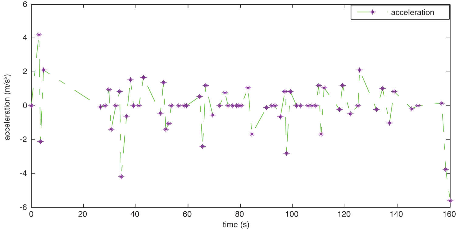
Figure 6: Acceleration curve of the ego-vehicle

To test the validity of ICV autonomous driving decision-making reported in Fig. 4, during the panoramic vision experiment we invited 10 experienced drivers to simultaneously appraise every driving decision made by the HFSM model. For every driving decision, the experienced driver gave a score {0, 1, 2, 3, 4, 5, 6} in line with a satisfactory grade {very unreasonable, unreasonable, reasonable, normal, suboptimal, optimal, very optimal}. Among all 66 driving decisions, the lowest and highest average scores are 3.40 and 5.70, respectively. Moreover, the average score of all 66 decisions is 3.97, higher than the normal level. This study also conducted a statistical test on hypothesis H0:μ≤3.0 for every decision. Fig. 7 reports that at a 5% significance level, every driving decision is better than the normal level; and at a 1% significance level, there are 39 driving decisions better than the normal level. Therefore, the HFSM model and TOPSIS-GRA algorithm are valid for ICV autonomous driving decision-making.

Figure 7: Statistical test on decision-making results

5.2 Collision Avoidance Simulation Results

This section provides a detailed explanation of the first collision avoidance scenario to illustrate how the HFSM model and TOPSIS-GRA algorithm work well for ICV autonomous driving decision-making. Fig. 8 depicts the traffic scenario and Table 1 provides the position and velocity of each vehicle.

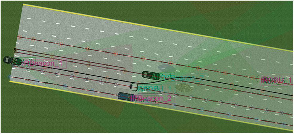
Figure 8: The first collision avoidance scenario

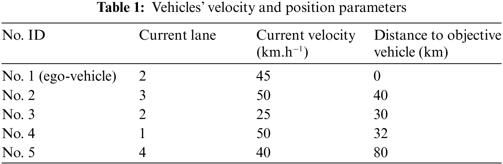
Table 2 displays the driving behavior decision-making matrix of the global FSM model. To obtain the subjective weight of events in the global FSM model, we invited 8 experienced drivers to rate the importance of events in Table 2 based on risky driving theory. Utilizing one-by-one comparison and bipolar scale method, they gave each event and upper layer index a score from set {1, 2 … 9}. By employing the AHP algorithm to deal with expert data, the subjective weight of events is obtained, as shown in Table 3. On the other hand, the objective weight of events is directly calculated by the EWM method according to data in Table 2.

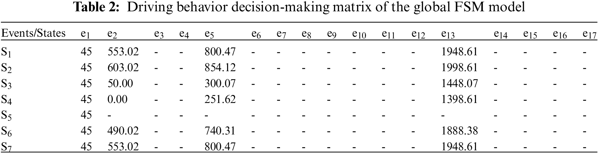
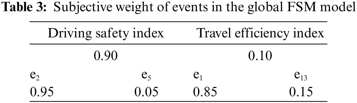
Table 4 reveals that when making a driving behavior decision for the first collision avoidance scenario, the global FSM output is On Road (S2) state, which is strictly following the ego-vehicle’s real traffic scenario displayed in Fig. 8. Note that, because the mission document does not find the state of field driving (S5), it is removed by matrix refining procedure and not reported in Table 4. To test the robustness of the TOPSIS-GRA algorithm, we randomly select 5 portfolios of AHP preference factor and TOPSIS preference coefficient, and then simulate the synthetic similarity degree of driving state in the global FSM model. Under each portfolio, the output of the global FSM model is still On Road (S2) state, as displayed in Fig. 9. It reveals that the global FSM model is controlled by driving characteristic events, and is robust relative to the change of AHP preference factor as well as TOPSIS preference coefficient.

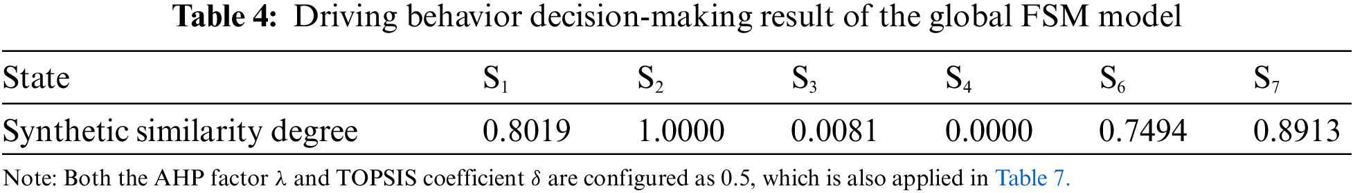
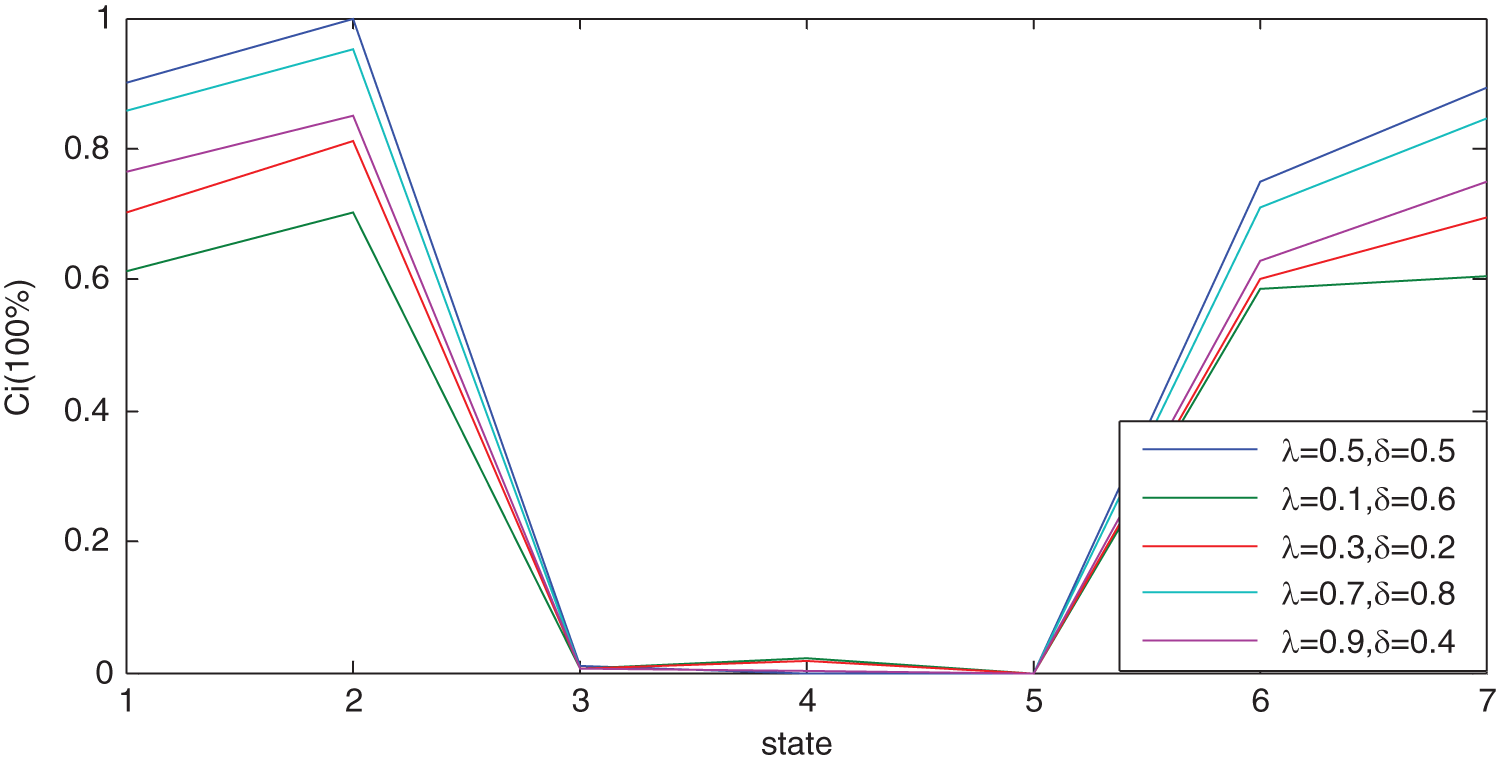
Figure 9: Outputs of the global FSM under different parameters

Table 5 is the driving behavior decision-making matrix of the local FSM model. Similar to the global FSM model, the 8 experienced drivers respectively rated the importance of each event and upper layer indexes through one-by-one comparison and bipolar scaling method. The subjective weight of events is obtained by employing the AHP algorithm to deal with expert data, as shown in Table 6. Also, the objective weight of events is obtained by directly employing the EWM algorithm to deal with data in Table 5.

As displayed in Table 7, the output of the local FSM model is state S11 (change to left lane with deceleration), which is well matched with the traffic scenario depicted in Fig. 8. Moreover, the 10 experienced drivers synchronously appraised this driving decision and gave an average score 3.7, higher than the normal level 3.0, which also verified the validity of driving decision made by the HFSM model.

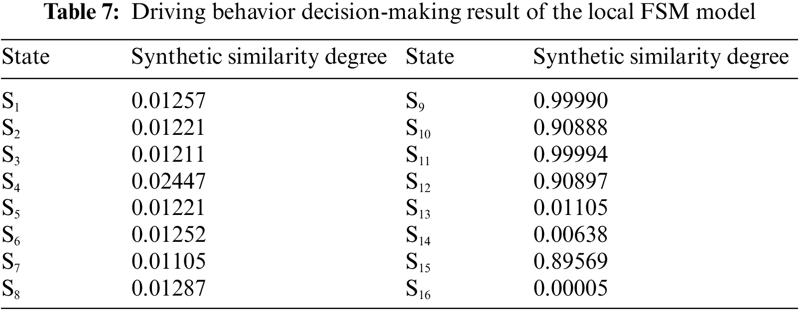
Fig. 10 reveals that under randomly selected 5 portfolios of AHP preference factor and TOPSIS preference coefficient, the driving decision result of the local FSM is still state S11. Also, it supports that the local FSM model is controlled by driving characteristic events, and has a robustness feature relative to the change of the AHP preference factor or TOPSIS preference coefficient. In addition, under different parameter portfolios, the synthetic similarity degree of state S9 is almost equal to that of state S11 in Fig. 10. The main reason is that under the current traffic scenario, the left forward vehicle (No. 2) has a higher speed than ego-vehicle, hence, the decision of change to left lane without deceleration (S9) is also feasible.

Figure 10: Local FSM output under different factors

Fig. 11 displays the effectiveness of ICV autonomous driving decision-making for the first collision avoidance scenario. Concerning main technical indicators, the path planning time of collision avoidance is 45 ms, the distance of lane line prediction gets 62.78 m, the maximum speed during collision avoidance reaches 45 km/h, and the shortest distance of collision avoidance is 4.3 m. Technically, these results may meet the requirements of ICV advanced autonomous driving under 5G-V2X intelligent road infrastructure.

Figure 11: Effectiveness of self-driving decision

6  Conclusions

5G-V2X technology makes it possible to control ICV autonomous driving in a real-time situation by fusing ICV and connected automated transport systems to synchronously analyze big data of current traffic scenarios. Based on cooperative environment perception technology and multi-source heterogeneous data fusion algorithm, ICV may have the ability to detect the environment outperforming that of an experienced driver, hence, it may realize a complete understanding of the current traffic scenarios.

This paper proposes an HFSM model as well as a TOPSIS-GRA algorithm for ICV autonomous driving decision-making under 5G-V2X road infrastructure, and further performs a series of simulative experiments in PreScan8.50 environment to test its feasibility, validity, safety, and robustness. The HFSM model contains two layers: global FSM and local FSM. The decision result of the former is one of input information of the latter. Meanwhile, the result of the latter produces feedback to the former to refresh input data simultaneously. Concerning different traffic scenarios, the global FSM model is comprised of 7 driving states and 17 characteristic events. Based on the global FSM output and different traffic scenarios, the local FSM model is comprised of 16 driving states and 8 characteristic events. The proposed TOPSIS-GRA algorithm firstly fuses subjective weight and objective weight to generate a synthetic weight of the driving event, thereafter, it fuses the TOPSIS and GRA ranking algorithms to get the implementable order of state transition. In line with PreScan8.50 simulative experiments on conditions of different traffic scenarios, the results support that the HFSM model’s states set, events set as well as state transition algorithm, can meet the requirements of ICV self-driving under 5G-V2X road infrastructure.

In technical terms, PreScan simulative experiments display that the accuracy of obstacles detection gets 98% through fusing multisource sensors data, lane line prediction beats 70 m, the speed of collision avoidance is higher than 45 km/h on linear lane conditions, the distance of collision avoidance is less than 5 m, path planning time for obstacle avoidance is averagely less than 50 ms, and brake deceleration is controlled under 6 m/s2. In general, the value of these indexes can satisfy technical conditions for ICV advanced autonomous driving.

When deciding on ICV autonomous driving, more driving states and characteristic events will bring about more accurate driving action as well as a higher intelligence level of the system. However, the complexity of the HFSM model may induce an overlap of trigger conditions and thus increase the time-latency of decision-making. In practice, since different driving behavior matrices in the HFSM model match different traffic scenarios, constructing a traffic scenario library may well promote ICV self-driving technology development. These two aspects can be a follow-up research direction of this paper.

Acknowledgement: This research was supported by Chongqing Science and Technology Bureau, Chongqing Education Commission, and Chongqing University of Arts and Sciences.

Funding Statement: This research was funded by Chongqing Science and Technology Bureau (No. cstc2021jsyj-yzysbAX0008), Chongqing University of Arts and Sciences (No. P2021JG13) and 2021 Humanities and Social Sciences Program of Chongqing Education Commission (No. 21SKGH227).

Conflicts of Interest: The authors declare that they have no conflicts of interest to report regarding the present study.

References

1. H. Bagheri, M. Noor-A-Rahim, Z. L. Liu, H. Lee, D. Pesch et al., “5G NR-v2X: Towards connected and cooperative autonomous driving,” IEEE Communications Standards Magazine, vol. 5, no. 1, pp. 48–54, 2021. [Google Scholar]
2. D. K. Ren and Z. S. Liao, “Research on application of 5G-v2X autonomous driving,” Telecom. Engineering Technics and Standardization, vol. 33, no. 09, pp. 68–74, 2020. [Google Scholar]
3. X. X. Jin, “Importance and key technology of C-v2X and trend of telecommunications technology,” China Internet, vol. 08, no. 4, pp. 25–34, 2020. [Google Scholar]
4. K. Alheeti, A. Alaloosy, H. Khalaf, A. Alzahrani, D. Al_Dosary, “An optimal distribution of RSU for improving self-driving vehicle connectivity,” Computers, Materials & Continua, vol. 70, no. 2, pp. 3311–33189, 2022. [Google Scholar]
5. J. B. Gao, “Research on decision-making and control method for autonomous vehicle,” M.S. Thesis, School of Jiaotong, Chongqing Jiaotong University, Chongqing, China, 2019. [Google Scholar]
6. Z. H. Gao, X. T. Yan, F. Gao and L. He, “Driver-like decision-making method for vehicle longitudinal autonomous driving based on deep reinforcement learning,” Proceedings of the Institution of Mechanical Engineers, Part D: Journal of Automobile Engineering, vol. 14, no. 12, pp. 3060–3070, 2021. [Google Scholar]
7. D. Gonzalez, M. Garzon, J. Dibangoye and C. Laugier, “Human-like decision-making for automated driving in highways,” in 2019 IEEE Int. Conf. on Intelligent Transport Systems, Auckland, New Zealand, pp. 1–8, 2019. [Google Scholar]
8. Y. Xia, Z. Qu, Z. Sun and Z. H. Li, “A human-like model to understand surrounding vehicles’ lane changing intentions for autonomous driving,” IEEE Transactions on Vehicular Technology, vol. 70, no. 5, pp. 4178–4189, 2021. [Google Scholar]
9. Z. Wang, W. Chen, P. Wang, M. Li, Y. Xin et al., “A decision-making model for autonomous vehicles at urban intersections based on conflict resolution,” Journal of Advanced Transportation, vol. 2021, no. 2, pp. 1–12, 2021. [Google Scholar]
10. Y. X. Chen, N. Sohani and H. Peng, “Modelling of uncertain reactive human driving behavior: A classification approach,” in CDC 2018 IEEE Conf. on Decision and Control, Miami, USA, pp. 3615–3621, 2018. [Google Scholar]
11. A. Gupta, A. Anpalagan, L. Guan and A. S. Khwaja, “Deep learning for object detection and scene perception in self-driving cars: Survey, challenges, and open issues,” Array, vol. 10, no. 3, pp. 1–20, 2021. [Google Scholar]
12. L. Danys, R. Martinek, R. Jaros, J. Baros, P. Simonik et al., “Enhancements of SDR-based FPGA system for V2X-VLC communications,” Computers, Materials & Continua, vol. 68, no. 3, pp. 3629–3651, 2021. [Google Scholar]
13. T. Sakuma, S. Miura, T. Miyashita, M. G. Fujie and S. Sugano, “Development of human-like driving decision making model based on human brain mechanism,” in 2019 IEEE/SICE Int. Symp. on System Integration (SII), Paris, France, pp. 770–775, 2019. [Google Scholar]
14. E. Seo, S. Lee, G. J. Shin, H. Yeo, Y. Lim et al., “Hybrid tracker based optimal path tracking system of autonomous driving for complex road environments,” IEEE Access, vol. 4, no. 2, pp. 1–15, 2016. [Google Scholar]
15. L. Li, W. Z. Zhao, C. Xu, C. Wang, Q. Y. Chen et al., “Lane-change intention inference based on RNN for autonomous driving on highways,” IEEE Transactions on Vehicular Technology, vol. 70, no. 6, pp. 5499–5510, 2021. [Google Scholar]
16. N. D. Van, M. Sualeh, D. H. Kim and G. W. Kim, “A hierarchical control system for autonomous driving towards urban challenges,” Applied Sciences, vol. 10, no. 10, pp. 1–26, 2020. [Google Scholar]
17. C. Y. Jung, D. Lee, S. Lee and D. H. Shim, “V2X-communication-aided autonomous driving: System design and experimental validation,” Sensors, vol. 20, no. 4, pp. 1–22, 2020. [Google Scholar]
18. X. Y. Zhang, H. B. Gao, M. Guo, G. P. Li, Y. C. Liu et al., “A study on key technologies of unmanned driving,” CAAI Transactions on Intelligence Technology, vol. 41, no. 1, pp. 4–13, 2016. [Google Scholar]
19. W. P. Lin, “Research on autonomous driving and key technologies of V2X,” Guangdong Communication Technology, vol. 38, no. 11, pp. 44–48, 2018. [Google Scholar]
20. P. Hang, C. Lv, C. Huang, Y. Xing, Z. X. Hu et al., “Human-like lane-change decision making for automated driving with a game theoretic approach,” in 2020 4th CAA Int. Conf. on Vehicular Control and Intelligence, CVCI 2020, Hangzhou, China, pp. 708–713, 2020. [Google Scholar]
21. L. Z. Li, K. Ota and M. X. Dong, “Humanlike driving: Empirical decision-making system for autonomous vehicles,” IEEE Transactions on Vehicular Technology, vol. 67, no. 8, pp. 6814–6823, 2018. [Google Scholar]
22. M. X. Zhang, N. Li, A. Girard and I. Kolmanovsky, “A finite state machine based automated driving controller and its stochastic optimization,” in ASME Dynamic Systems and Control Conf., Tysons, USA, pp. 1–10, 2017. [Google Scholar]
23. A. Kurt and U. Ozguner, “Hierarchical finite state machines for autonomous mobile systems,” Control Engineering Practice, vol. 21, no. 2, pp. 184–194, 2013. [Google Scholar]
24. X. Y. Wang, X. D. Qi, P. Wang and J. W. Yang, “Decision making framework for autonomous vehicles driving in complex scenarios via hierarchical state machine,” Autonomous Intelligent Systems, vol. 1, no. 10, pp. 1–10, 2021. [Google Scholar]
25. P. Wang, S. Gao, L. Li, S. Cheng and H. Zhao, “Research on driving behavior decision making of autonomous driving vehicle based on benefit evaluation model,” Archives of Transport, vol. 53, no. 1, pp. 21–36, 2020. [Google Scholar]
26. D. Sales, D. Correa, L. Fernandes, D. Wolf and F. Osorio, “Adaptive finite state machine based visual autonomous navigation system,” Engineering Applications of Artificial Intelligence, vol. 29, no. 2, pp. 152–162, 2014. [Google Scholar]
27. H. Raza and P. Loannou, “Vehicle following control design for automated highway systems,” IEEE Control Systems Magazine, vol. 1, no. 6, pp. 43–60, 1996. [Google Scholar]
28. G. S. Wilde, “Social interaction patterns in driver behavior: An introductory review,” Human Factors: The Journal of the Human Factors and Ergonomics Society, vol. 18, no. 5, pp. 477–492, 1976. [Google Scholar]
29. P. Hang, C. Lv, Y. Xing, C. Huang and Z. X. Hu, “Human-like decision making for autonomous driving: A noncooperative game theoretic approach,” IEEE Transactions on Intelligent Transportation Systems, vol. 22, no. 4, pp. 2076–2087, 2021. [Google Scholar]
30. B. R. Andrievsky and A. L. Fradkov, “Speed gradient method and its applications,” Automation and Remote Control, vol. 82, no. 10, pp. 1463–1518, 2021. [Google Scholar]
31. M. X. Zu, Y. H. Wang, Z. Y. Pu, J. Y. Hu, X. S. Wang et al., “Safe, efficient and comfortable velocity control based on reinforcement learning for autonomous driving,” Transportation Research Part C: Emerging Technologies, vol. 117, no. 8, pp. 1–8, 2020. [Google Scholar]
32. Z. Constantinescu, C. Marinoiu and M. Vladoiu, “Driving style analysis using data mining techniques,” International Journal of Computers, Communications & Control, vol. 5, no. 5, pp. 654–663, 2010. [Google Scholar]
33. C. Wang, Q. Y. Sun, Z. Li and H. J. Zhang, “Human-like lane change decision model for autonomous vehicles that considers the risk perception of drivers in mixed traffic,” Sensors, vol. 20, no. 8, pp. 1–20, 2020. [Google Scholar]
34. ISO 15623, “Intelligent transport systems-forward vehicle collision warning systems-performance requirements and test procedures,” Switzerland, ISO, 2013. [Online]. Available: https://library.precious-plastic.org/documents/isos/15001-20000/ISO%2015623-2013.pdf. [Google Scholar]
35. J. Y. Cao, H. Lu, K. H. Guo and J. W. Zhang, “A driver modeling based on the preview-follower theory and the jerky dynamics,” Mathematical Problems in Engineering, vol. 2013, no. 6, pp. 1–10, 2013. [Google Scholar]
36. S. Zhong, M. Wei, S. Gong, K. Xia, Y. Fu et al., “Behavior prediction for unmanned driving based on fusion of feature and decision,” IEEE Transactions on Intelligent Transportation System, vol. 22, no. 6, pp. 3687–3696, 2021. [Google Scholar]
Cite This Article
Copyright © 2023 The Author(s). Published by Tech Science Press.
This work is licensed under a Creative Commons Attribution 4.0 International License , which permits unrestricted use, distribution, and reproduction in any medium, provided the original work is properly cited.
Downloads
Citation Tools