Short Term Traffic Flow Prediction Using Hybrid Deep Learning

1  Introduction

STTF forecasting is based on actual and past transit information recorded from sensing devices, namely cameras, radar, and inductors. The extensive use of traffic sensors and the modernization of extending traffic sensing devices largely boost the traffic flow data. In extensive data transit, data-driven mobility management and monitoring became increasingly widespread. Accurate and precise traffic flow data reduces traffic congestion, enhances traffic operation efficiency, and optimizes travel decisions. Effective and accurate traffic flow forecast is critical research in Intelligent Transportation Systems. It not only assists traffic managers in anticipating traffic operations and avoiding potential traffic congestion but also offers more traffic information, allowing travelers to plan their trips before time and adjust their routes [1]. Across the globe, people are adopting ITS to save on the costs associated with traffic. Traffic flow prediction has consistently been regarded as a practical focus in ITS. STTF forecast is an essential issue regarding ITS. Exact traffic flow prediction models were significant to lesser traffic, preventing pollution, and facilitating strategic decisions by sovereignty [2]. ITS integrates data collection, knowledge acquisition, mechanization, and other capabilities to allocate mobility and accessibility to less traffic effectively. On the other hand, travel demands have been developed over recent years, supporting traffic management, controlling traffic performance, extending route assistance, and vehicle scheduling for signal cooperation [3]. Transit Research and Development was restricted through environmental, automated, enterprise exploration, and specific extant technology. However, traffic is wreaking havoc on the world’s exterior road infrastructure. In the present era, ITS is more challenging to enhance traffic efficiency and safety. For mobility design and planning reviews, traffic flow prediction (TFP) would be necessary. Traffic Flow Prediction examines the traffic flow to estimate future traffic patterns, and projections might be separated into two categories: short-term and long-term. For example, a time interval of less than an hour is generally considered short-term or medium, and more than an hour is considered long-term [4]. Monitoring road traffic is feasible and broadly depends on the framework or computation, internal or external, and parametric model or non-parametric model. This provides brief ideas for intelligent city management systems and priority transportation management. During the past generations, various academic papers mainly emphasized the ITS and data analysis. In the later part of the 1980s, short-term traffic forecasting was a significant area related to the ITS. It refers to forecasts that range between just a few minutes to several hours in forthcoming, with current and historical traffic data. Predictive analytics for urban transit are relevant in the ITS with significant facets. Administration and transit authorities may help to understand citizens’ concerns identify traffic patterns and fix problems by evaluating internet community facts. Data analytics enables transportation agencies to focus on crucial concerns by sorting down the non-essential information [5].

The general augmentation concerning this article seems to be hereunder.

1.    We introduced PCA to remove unwanted information from the dataset and select essential features.

2.    We introduced SAE to reduce the dimension of input data. So the input data has high visibility to the model for faster execution with less time because of one hot representation.

3.    LSTM model will derive a value by considering 100 initial one-hot values as input data.

4.    All the Derived values of LSTM will be given to KNN to predict the final traffic flow using the mean of K Nearest Neighbors (where k = 5) with the help of Euclidean Distance optimizer.

5.    We calculated overall work using PALKNN through statistics. We regulated PALKNN at the actual dataset and tested the outcomes demonstrating the effectiveness of PALKNN, which seems to be preferable to other forecasting approaches.

2  Literature Review

The first research regarding STTF prediction was conducted during the 1980s. Short-term traffic flow forecasting predicts traffic from several minutes to hours in the long run, using present and historical data. In recent times, extensive work has been carried out on this issue. Existing traffic flow prediction techniques can be broadly divided into two categories: the parametric model and the non-parametric model.

2.1 Parametric Model

The Auto-Regressive Integrated Moving Average (ARIMA) framework was developed in the late 1970s, which proposes to forecast precise road transport flow Seasonal Auto-Regressive Integrated Moving Average (SARIMA) multivariate time series models and spectral analysis. Kumar et al. [6] developed a Short Term Traffic Flow forecast supported by Seasonal ARIMA (SARIMA) model. During the last several decades, Complex nonlinear methodologies and algorithms for traffic flow prediction have evolved.

Voort et al. [7] proposed the Kohonen Auto-Regressive Integrated Moving Average (KARIMA) approach, a hybrid method of short-term traffic forecasting that is like a preliminary encoder; the method utilizes a Kohonen self-organizing map for each class having its own experience and ARIMA model. The challenge of specifying the categories is made more accessible by using a hexagonal Kohonen map when contrast to a single ARIMA model or a backpropagation neural network.

Zhang et al. [8] proposed a hybrid model for multi-step forward traffic flow forecasts that decays the data into three models: an intraday or cyclic trend, a stochastic part simulated by the ARIMA model, and instability assessed by the Glosten Jagannathan Runkle-Generalized AutoRegressive Conditional Heteroskedasticity (GJR-GARCH) model. This model gains a better understanding of traffic patterns and enhances prediction accuracy and reliability by modeling them individually.

2.2 Non-Parametric Model

Wei et al. [9] offer a novel traffic flow prediction technique known as Auto Encoder Long Short-Term Memory (AE-LSTM) that leverages the Auto Encoder clipping a significant correlation between transit outflows via collecting all aspects regarding downstream plus upstream transit outflow knowledge. Cheng et al. [10] present a traffic flow prediction approach that relies on chaos theory. Traffic flow patterns such as speed, occupancy, and flow utilize the Lyapunov parameter and the Support Vector Regression (SVR) approach, often used to predict traffic flow in the big data environment. Chen [11] introduced an enhanced forecasting model premised on kernel function positioned Artificial Bee Colony (ABC) design, which regulates radial basis function (RBF) neural network weights & target values often used to examine nonlinear time sequences.

Farahani et al. [12] developed a Variational Long Short Term Memory Encoder (VLSTM-E) forecast approach, which reflects short-term traffic flow by considering the dispersal and incomplete data. Spatio-temporal Recurrent Convolutional Networks (SRCNs) introduced by Yu et al. [13] retain the benefits of Deep Convolutional Neural Networks (DCNN) in catching the spatial dependencies of network-wide traffic as well as simulated neural networks with Long Short Term Memory in working temporal dynamics.

Polson et al. [14] developed a Deep Learning model to forecast traffic flows. The key focus would be the design of a layout that integrates mathematical patterns with smoothing a series of elements. Hou et al. [15] developed a Linear Auto-regressive Integrated Moving Average (LARIMA) strategy as well as a nonlinear Wavelet Neural Network (WNN) hybrid model; the results of two individual methods were examined and integrated using fuzzy logic, with the weighted outcome serving as the hybrid model is anticipating the final traffic volume. Wu et al. [16] introduced a Deep Neural Network Based Traffic flow (DNN-BTF) prediction framework that involves massive utilization of weekly or daily basis and spatial-temporal traffic flow parameters to enhance accuracy rate.

Zheng et al. [17] suggested Sparse Regression forecasting models which can reliably and efficiently incorporate Spatial-Temporal factors. Aqib et al. [18] proposed a multifaceted approach to a vehicular assumption at a massive ratio instantaneously besides integrating four parallel innovations; huge information, expert systems, data processing, and graphics processing unit. Duhayyim et al. [19] introduce an Artificial Intelligence Traffic Flow Prediction with Weather Conditions (AITFP-WC) for smart cities. The Elman Neural Network (ENN) method is an aspect of the proposed AITFP-WC technique and is used to forecast traffic flow in smart cities. The weather and periodicity review also uses the Tunicate Swarm algorithm with the Feed-Forward Neural Networks (TSA-FFNN) model. Yan et al. [20] proposed a novel least squares twin support vector regression method based on the robust L1-norm distance to mitigating traffic data’s negative impact with outliers. An iterative approach is designed to overcome non-smooth L1-norm terms; its convergence is also revealed. Yan et al. [21] recommended three improved least squares twin support vector regression methods based on robust L1-norm, L2 p-norm, and Lp-norm distance to mitigating negative traffic data impact with outliers pruning scheme was also used to eliminate abnormal components.

Shu et al. [22] presented the Gated Recurrent Unit (GRU) model to extract the spatial and temporal characteristics of the flow matrix; an improved GRU with a bidirectional positive and negative feedback called the bidirectional-Gated Recurrent Unit (Bi-GRU) prediction model used to complete the short-term traffic flow prediction and study its characteristics. Finally, the Rectified Adaptive (RAdam) model is adopted to improve the shortcomings of the typical optimizer. Li et al. [23] introduce a new deep-learning Generative Adversarial Capsule Network (GACNet) architecture for predicting regional epitaxial traffic flow. GACNet forecasts traffic flow in surrounding areas based on data on inflow and outflow in the city center. The data-driven approach distinguishes the spatial relationship by adaptively converting traffic data into images via a two-dimensional matrix.

3  PALKNN Method

3.1 Methodology

Therefore in this section, we build a PALKNN method for analyzing the short-term traffic flow prediction exhibited in below Fig. 1. Additional details of the proposed PALKNN architecture are presented in the following subsections.

Figure 1: PALKNN architecture

3.1.1 Principal Components Analysis

PCA is an unsupervised algorithm used to minimize the attribute strategy. It cleans up data sets so they can be explored and analyzed more easily. A data set has many attributes that refer to the dimensions of the data set. Parameter removal is the technique of reducing attribute space by removing features. The drawback would be that the data related to the variables are lost. Insignificant attributes have been removed from the data set by PCA. PCA approach combines the concepts of the covariance matrix, eigenvectors, and eigenvalues. We must decide which attributes from the dataset to retain with further analysis; because each eigenvalue roughly represents the significance of its correlating eigenvector, the variance proportion revealed is the sum of the eigenvalues of the attribute divided by the sum of eigenvalues of all features Eq. (1). We can eliminate the eigenvectors that are relatively less significant using PCA. The mathematical equation of PCA is hereunder [24].

X.A=δ.A(1)

where

X-denotes n * n parent square,

A-denotes the eigenvector of the matrix,

δ-denotes the eigenvalue scalar.

3.1.2 Stacked Auto-Encoder

SAE is a kind of unsupervised model. The SAE reduces the data dimension by retaining attributes to reconstruct the data using one hot encoding (OHE). OHE is a binary vector description of categorical variables. OHE is the process of reducing binary categorical data into N columns of binary 0’s and 1’s with ‘N’ distinct groups, where 1 in the ‘N’th category implies the assessment relates to that category using the Scikit-Learn. OHE has an encoding function that begins with the shape of the input data. The decoding layer then takes that embedding and expands it back to the original shape. Finally, we bring the reconstruction from the decoder and calculate the reconstruction’s loss Eq. (2) vs. the original input [25].

L(Y,Y′)=||Y−Y′||=||(Y−σ′(W′(σ(WY+b))+b′))||2(2)

where

Y-denotes the original input

Y’-denotes the reconstructed input

σ-denotes the activation function

σ′-denotes the loss function

W-denotes the weight

b–denotes the bias

3.1.3 Long Short Term Memory

LSTM endures a Recurrent Neural Network regularly used in Artificial Intelligence Applications for analyzing and predicting time series data. However, LSTM assists in resolving Vanishing Gradient or Exploding Gradient errors, and also LSTM helps mitigate the Past Information Carry Forward problem. LSTM is trained through time using Backpropagation that resolves the vanishing gradient problem. The primary objective of LSTM cells is to remember the sequence components while ignoring the less crucial components. LSTM networks use memory blocks linked together in layers rather than neurons. A block contains components that enable it to be more intelligent than a traditional neuron and to remember recent sequences. A block includes gates that regulate the block’s state and output. A block performs on input sequence; every gate inside a block utilizes the sigmoid activation units to regulate whether it is triggered or not, making the deviation of state and addition of data exchange via block constraint. There are three kinds of gates, namely Forget Gate, Input Gate, and Output Gate, defined below sections [26]. LSTM Neuron architecture exhibits in below Fig. 2.

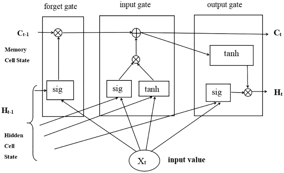
Figure 2: LSTM neuron architecture

Forget Gate

Forget Gate endures in charge of determining the information from the previous phase should be discarded. Eq. (3) defines the sigmoid layer. Thus it determines a range against 0 to 1 as all value cell states Ct-1 according to ht-1 (initial hidden state) and xt (present input at time-step t). The content has been maintained for all 1 s, the complete range is discarded for all 0 s, and other values determine more input from the previous state should be passed over to the next state.

dt=σ(Wf⋅[ht−1,xt]+bf)(3)

where

σ-denotes the sigmoid stimulation task (converts input into 0 to 1),

Wf-denotes the weights,

ht−1,xt-denotes the input,

bf-denotes the bias.

Input Gate

The input gate layer determines the updated values. A tanh component subsequently generates variables regarding future prospective principles in Eq. (4). Integrating those input gates within the following stage towards making state upgrades. Now, it is the time to shift from decrepit cell state Ct-1 towards the modern cell state Ct. Increasing the initial state besides xt in Eq. (5), ignoring the elements previously decided to forget.

it=σ(Wi⋅[ht−1,xt]+bi)(4)

C~t=tanh(Wc⋅[ht−1,xt]+bc)(5)

where

tanh-denotes the activation function,

Wc-denotes the weights,

ht−1,xt-denotes the input,

bc-denotes the bias.

Cell State

LSTM memory is the state of cells. While working on longer sequences of input, it exceeds vanilla Recurrent Neural Networks throughout this state. For every earlier time, the phase cell state Ct-1 combines with the forget gate to determine the input to move forward, which further interacts with the input gate by creating the storage or advanced cell state.

Output Gate

The output gate depends on the cell state in Eq. (6), which will be extracted. Next, execute a sigmoid layer used to calculate how each element of such cell state seems to be efficient. Finally, the cell state has been forwarded via tanh (ensure the principles toward being among −1 and 1) and magnified output through the sigmoid gate in Eq. (7).

ot=σ(Wo[ht−1,xt]+bo)(6)

ht=ot∗tanh(Ct)(7)

where

σ-denotes the sigmoid activation function,

Wo-denotes the weights,

bo-denotes the bias,

Ct-denotes the cell state.

3.1.4 K-Nearest Neighbors

KNN is a supervised machine learning algorithm that can perform both regression and classification problems. KNN is applied to predict outcomes on the test data according to the properties of the existing training data points. For example, the distance between the testing and training data is calculated. The KNN algorithm will discover its properties/attributes when adding a new data point. It will then move the new data point closer to the existing training data points that share the same features. To classify new data points, KNN computes the distance between them. Euclidean is the most commonly used technique for calculating this distance [27]. Euclidean distance is the length of a line linking two points employed to compute the distance between them. The method for Euclidean Distance is the square root of the sum of the squared differences between a new data point (a) and an existing trained data point (b) in Eq. (8).

∑j=1n(aj−bj)2(8)

4  Implementation

4.1 Time-Series Data

The times-series data frame to LSTM is then transformed using the time-series data structure frame considered in the proposed model for LSTM. This data frame was prepared after removing all the unwanted features in the UK traffic dataset by PCA technique which is an automation process, unlike manual, and after converting the data into one hot representation by SAE. Generally, Dt1 will be the one hot representation of all_motor_vehicles at the t1 time frame. Such ten one-hot representation of all_motor_vehicles at different sequential time frames sorted based on date, time, and travel direction were considered in ascending order to derive the Dt11. Times-series data frame to LSTM is hereof in Table 1.

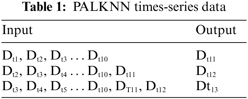
DtN is the traffic data at the Nth time frame where N > 0.

4.2 Algorithm

Pseudo Code of PALKNN

-----------------------------------------------------------------------------------------------------------------------

Input: UK Traffic dataset.

Output: Traffic flow

-----------------------------------------------------------------------------------------------------------------------

1.   Load the UK traffic Dataset [From 2000–2020]

2.   Apply Data Preprocess activities like

Input Data Preparation:

3.   Add StandardScalarization transform technique with a range between −1 and 1.

4.   Add PCA instance with retaining ability as 99%.

5.   Add reverse StandardScalarization.

6.   StackedAutoEncoder:

7.   Sort the dataset based on count_date, hour, and direction_of_travel columns.

8.   Considering only the all_motor_vehicles column to prepare the time series (Sequential) dataset,

9.   LSTM Times-series Data [Table 1].

Model Construction:

10.   Create a Sequential model with

11. Fit or Train the Model with input data for 275 epochs and capture the loss.

12. Predict traffic flow.

-------------------------------------------------------------------------------------------------------------------------

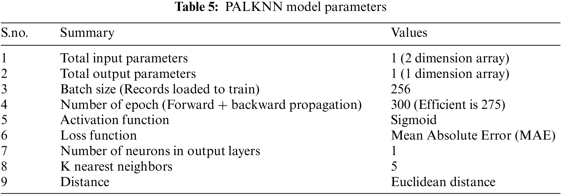
The parameter configuration of PCA, SAE, LSTM, and KNN are shown below in Tables 2–5, respectively.

5  Experiments and Results Analysis

5.1 Data Description

In this work, the traffic flow dataset was collected from zone 1 to zone 5 Department of Transport, Great Britain, United Kingdom (UK) [28]. This dataset is a skilled attainment method; the detectors were used to record automobile statistics on major and minor highways in Great Britain, UK. Utilizing 8,000 highway physical observations, the electronic vehicle monitors capture the pertinent data. This dataset was used for the experimental analysis to contrast with other algorithms. The author used the PALKNN model to test its effectiveness using real datasets of traffic data obtained over 20 years (2000–2020), in which the dataset contains 31 attributes with Spatio-temporal data such as rain, snowfall, and windy seasons because these factors impact traffic flow a lot during weekdays.

In this experiment, the data set was divided into two parts with ratios of 75% for the training dataset and 25% for the testing dataset. In addition, there is a feature or column called all_motor_vehicles. This feature comprises a count of pedal cycles, two-wheeled motor vehicles, cars, taxis, buses, coaches, Light Goods Vans, two-rigid axle Heavy Goods Vans, three-rigid axle Heavy Goods Vans, four or more rigid axle Heavy Goods Vans, articulated axle Heavy Goods Vans of all weekdays and week off during both busy, quite periods.

5.2 Data Pre-Processing

However, at the initial stage, the proposed PALKNN model involves data pre-processing to standardize the input data using the standardschalarization approach from the scikit library. Standardization is a scaling technique that centers values on the mean with a unit standard deviation; this signifies that the attribute’s mean becomes zero and the resulting distribution has a unit standard deviation. In this work, the prior traffic flow of an hour, i.e., a PALKNN time series data is considered. PALKNN time series data used for training and testing in this intent.

5.3 Validation

The performance evaluation of STTF models tested with the work using three indexes; Root Mean Square Error (RMSE), shown in Eq. (9), Mean Square Error (MSE) as shown in Eq. (10), and Mean Absolute Error (MAE) as shown in Eq. (11) was evaluated [29]. The formulas are hereof:

RMSE=1n∑j=1n(e¯j−ej)2(9)

MSE=1n∑j=1n(ej−e¯j)2(10)

MAE=1n∑j=1n|e¯j−ej|(11)

where e¯j constitutes the predicted value, ej constitutes the observed value and n constitutes the number of data elements.

5.4 Results Analysis

To authenticate the validity of the proposed model, contrast it with five models: the KNN model, SARIMA model, Logistic Regression model, Recurrent Neural Network (RNN) model, and LSTM model using the UK traffic dataset. The error performance of training and testing models is shown below in Table 6.

After segregating the UK traffic dataset into training and testing data sets with a ratio of 75% and 25%, respectively, the proposed model was trained on a training data set and tested on both training and testing data sets; the loss rate in the testing data set reduced from 60% to 5% and the training data set from 53% to 5% as the epochs (training loops) increased. There were four convergences between training loss and testing loss at epoch 69, 100, 150, and 270, respectively, with loss rates of 52%, 31%, 30%, and 7%. Later, training loss reached 4%, and testing loss reached 6% before possible divergence began. The proposed model loss is around 6%, which is shown below in Fig. 3.

Figure 3: Loss of proposed algorithm on UK traffic data per epoch

The assessment between predicted traffic and actual traffic per hour of a day is shown in below Fig. 4. Here, predicted traffic indicates the proposed model prediction. The traffic flow is high in the morning peak hours between 6:00 and 11:30 am and evening peak hours between 16:05 and 22:05 pm. Traffic flow is moderate in off-peak hours. Therefore, the proposed model prediction is almost the same as the actual traffic flow except for a few hours; the predicted traffic is slightly higher and lower than actual traffic with a negligible difference.

Figure 4: Proposed algorithm traffic flow prediction

The estimation of predicted traffic with different models such as PALKNN, LSTM, RNN, Logistic Regression, SARIMA, and KNN is shown below in Fig. 5. It is clear that PALKNN prediction is the same and matches with the actual traffic most of the time, whereas other algorithms are far away from the actual traffic because their error rates are more significant than the proposed model error rate. So PALKNN is performing better than other techniques in traffic prediction.

Figure 5: All algorithms traffic flow prediction evaluation

Similarly, while training the proposed hybrid model, PALKNN achieved 3.5%, 1.8%, and 1.9% error values for RMSE, MSE, and MAE, whereas LSTM is 4%, and other algorithms are above 5%. Also, the proposed technique has a 3.5% MSE error value but all peer competitive techniques possess above 5%. So we concluded that the PALKNN hybrid model has less error rate in training shown in above Fig. 6.

Figure 6: Training RMSE, MSE, MAE on UK traffic data

Likewise, testing the proposed hybrid model PALKNN has negligible RMSE, MSE, and MAE error values as 4.1%, 2.04%, and 2.07%, respectively. However, for other techniques, it is above 4%. Even in testing, we have identified that the proposed algorithm is performing better with less error rate shown below in Fig. 7.

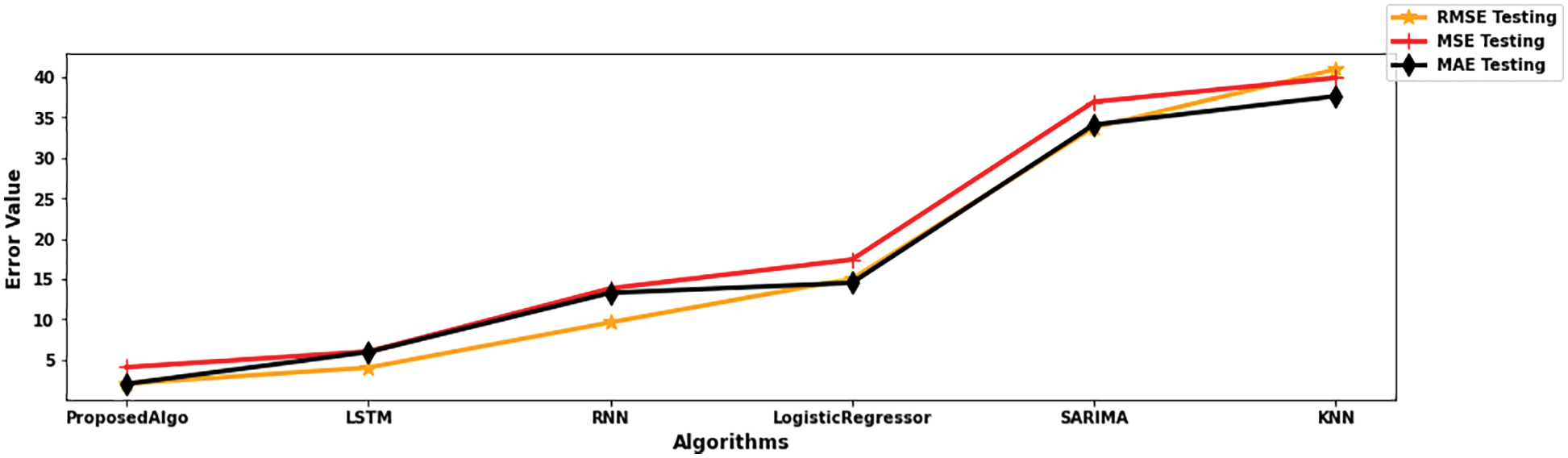
Figure 7: Testing RMSE, MSE, MAE on UK traffic data

There is no accuracy measuring metrics for regressor techniques, unlike classifiers, because in classifiers, we have defined several outputs (like True or False, Yes or No, 0 or 1, high or Low). In contrast, in regressor techniques, the output will be a real number ranging from −ve ∞ to +ve ∞ ∞ (Negative Infinity to Positive Infinity). Due to this output predicting the behavior of regressor techniques, we use the error rates to assess the performance. So if the error ratio is between 1% and 25%, then the regressor model would be the best fit for the business problem statement for the chosen data set.

In this research, the proposed model is a Regressor because the output layer contains a KNN regressor to predict the traffic flow value. We concluded that the proposed model is the best fit for the short-term traffic flow prediction because RMSE, MSE, and MAE ratios are less than 5% in both training and testing data sets, though other models values are less than 25% shown in the above Figs. 6 and 7.

6  Conclusion and Future Work

This work proposes an STTF prediction model PALKNN based on ensemble learning of PCA, SAE, LSTM, and KNN. PCA selects important features from the dataset. SAE performs dimensionality reduction using one-hot representation, converting the data into 0 and 1 s. So PCA and SAE prepare well-defined and highly visible input data to LSTM for faster execution; now LSTM takes sorted input in ascending order and generates the derived values. The KNN takes these derived values to predict traffic flow values. Finally, the proposed hybrid model PALKNN internally uses the optimizer called Euclidean Distance (which is the mean of K nearest neighbors, where k = 5) present in KNN to improve the performance by reducing the error rate. The research approach mainly focuses on the STTF prediction for every hour of a day, which is more efficient for commuters to plan their journeys. Finally, the performance of the PALKNN prediction model was validated using an actual data set from the road traffic statistics, UK. The metric findings below show that the proposed algorithm outperformed existing approaches such as KNN, SARIMA, Logistic Regression, RNN, and LSTM models.

•   Traffic prediction is more reliable and very similar to the actual value, with quicker execution when corresponding with other models.

•   Fewer error rates for RMSE, MSE, and MAE in testing data with values as 2.07%, 4.1%, and 2.04%, respectively.

•   Fewer error rates for RMSE, MSE, and MAE in training data with values as 1.9%, 3.5%, and 1.8%, respectively.

In future work, to make the traffic flow prediction more stable, the proposed PALKNN Regressor algorithm will be replaced with the PALKNN Classifier (both LSTM and KNN as classifiers) having two class labels such as HIGH and LOW traffics.

Funding Statement: The authors received no specific funding for this study.

Conflicts of Interest: The authors declare that they have no conflicts of interest to report regarding the present study.

References

1. Z. Cui, B. Huang, H. Dou, G. Tan and S. Zheng et al., “GSA-ELM: A hybrid learning model for short-term traffic flow forecasting,” IET Intelligent Transport Systems, vol. 6, no. 1, pp. 41–52, 2022. [Google Scholar]
2. W. Chen, J. An, R. Li, L. Fu and G. Xie et al., “A novel fuzzy deep-learning approach to traffic flow prediction with uncertain spatial–temporal data features,” Future Generation Computer Systems, vol. 89, pp. 78–88, 2018. [Google Scholar]
3. J. Mena-Oreja and J. Gozalvez, “A comprehensive evaluation of deep learning-based techniques for traffic prediction,” IEEE Access, vol. 8, pp. 91188–91212, 2020. [Google Scholar]
4. J. Guo, W. Huang and B. M. Williams, “Adaptive kalman filter approach for stochastic short-term traffic flow rate prediction and uncertainty quantification,” Transportation Research Part C: Emerging Technologies, vol. 43, no. 1, pp. 50–64, 2014. [Google Scholar]
5. W. Huang, G. Song, H. Hong and K. Xie, “Deep architecture for traffic flow prediction: Deep belief networks with multitask learning,” IEEE Transactions on Intelligent Transportation Systems, vol. 15, no. 5, pp. 2191–2201, 2014. [Google Scholar]
6. S. V. Kumar and L. Vanajakshi, “Short-term traffic flow prediction using seasonal arima model with limited input data,” European Transport Research Review, vol. 7, no. 3, pp. 1–9, 2015. [Google Scholar]
7. M. V. D. Voort, M. Dougherty and S. Watson, “Combining kohonen maps with arima time series models to forecast traffic flow,” Transportation Research Part C: Emerging Technologies, vol. 4, no. 5, pp. 307–318, 1996. [Google Scholar]
8. Y. Zhang, Y. Zhang and A. Haghani, “A hybrid short-term traffic flow forecasting method based on spectral analysis and statistical volatility model,” Transportation Research Part C: Emerging Technologies, vol. 43, no. 1, pp. 65–78, 2014. [Google Scholar]
9. W. Wei, H. Wu and H. Ma, “An auto encoder and lstm based traffic flow prediction method,” Sensors, vol. 19, no. 13, pp. 2946, 2019. [Google Scholar]
10. A. Cheng, X. Jiang, Y. Li, C. Zhang and H. Zhu, “Multiple sources and multiple measures based traffic flow prediction using the chaos theory and support vector regression method,” Physica A: Statistical Mechanics and its Applications, vol. 446, pp. 422–434, 2017. [Google Scholar]
11. D. Chen, “Research on traffic flow prediction in the big data environment based on the improved RBF neural network,” IEEE Transactions on Industrial Informatics, vol. 13, no. 4, pp. 2000–2008, 2017. [Google Scholar]
12. M. Farahani, M. Farahani, M. Manthouri and O. Kaynak, “Short-term traffic flow prediction using variational LSTM networks,” arXiv preprint arXiv: 2002.07922, 2020. [Google Scholar]
13. H. Yu, Z. Wu, S. Wang, Y. Wang and X. Ma, “Spatial-temporal recurrent convolutional networks for traffic prediction in transportation networks,” Sensors, vol. 17, no. 7, pp. 1501, 2017. [Google Scholar]
14. N. G. Polson and V. O. Sokolov, “Deep learning for short-term traffic flow prediction,” Transportation Research Part C: Emerging Technologies, vol. 79, no. 1, pp. 1–17, 2017. [Google Scholar]
15. Q. Hou, J. Leng, G. Ma, W. Liu and Y. Cheng, “An adaptive hybrid model for short-term urban traffic flow prediction,” Physica A: Statistical Mechanics and its Applications, vol. 527, pp. 121065, 2019. [Google Scholar]
16. Y. Wu, H. Tan, L. Qin, B. Ran and Z. Jiang, “A hybrid deep learning based traffic flow prediction method and its understanding,” Transportation Research Part C: Emerging Technologies, vol. 90, pp. 166–180, 2018. [Google Scholar]
17. Z. Zheng, L. Shi, L. Sun and J. Du, “Short-term traffic flow prediction based on sparse regression and spatio-temporal data fusion,” IEEE Access, vol. 8, pp. 142111–142119, 2020. [Google Scholar]
18. M. Aqib, R. Mehmood, A. Alzahrani, I. Katib, A. Albeshri et al., “Smarter traffic prediction using big data, in-memory computing, deep learning and GPUs,” Sensors, vol. 19, no. 9, pp. 2206, 2019. [Google Scholar]
19. A. I. Duhayyim M, A. A. Albraikan, F. N. A. I. Wesabi, H. M. Burbur, M. Alamgeer et al., “Modeling of artificial intelligence based traffic flow prediction with weather conditions,” Computers, Materials & Continua, vol. 71, no. 2, pp. 3953–3968, 2022. [Google Scholar]
20. H. Yan, Y. Qi and D. J. Yu, “Short-term traffic flow prediction based on a hybrid optimization algorithm,” Applied Mathematical Modelling, vol. 102, pp. 385–404, 2022. [Google Scholar]
21. H. Yan, L. Fu, Y. Qi, D. J. Yu and Q. Ye, “Robust ensemble method for short-term traffic flow prediction,” Future Generation Computer Systems, vol. 133, pp. 395–410, 2022. [Google Scholar]
22. W. Shu, K. Cai and N. N. Xiong, “A short-term traffic flow prediction model based on an improved gate recurrent unit neural network,” IEEE Transactions on Intelligent Transportation Systems, vol. 23, no. 9, pp. 16654–16665, 2022. [Google Scholar]
23. J. Li, H. Li, G. Cul, Y. Kang and Y. Hu et al., “Gacnet: A generative adversarial capsule network for regional epitaxial traffic flow prediction,” Computers, Materials & Continua, vol. 64, no. 2, pp. 925–940, 2020. [Google Scholar]
24. B. M. Salih Hasan and A. M. Abdulazeez, “A review of principal component analysis algorithm for dimensionality reduction,” Journal of Soft Computing and Data Mining, vol. 2, no. 1, pp. 20–30, 2021. [Google Scholar]
25. A. Moussavi Khalkhali and M. Jamshidi, “Feature fusion models for deep autoencoders: Application to traffic flow prediction,” Applied Artificial Intelligence, vol. 33, no. 13, pp. 1179–1198, 2019. [Google Scholar]
26. S. Hochreiter and J. Schmidhuber, “Long short-term memory,” Neural Computation, vol. 9, no. 8, pp. 1735–1780, 1997. [Google Scholar]
27. H. Yu, N. Ji, Y. Ren and C. Yang, “A special event-based k-nearest neighbor model for short-term traffic state prediction,” IEEE Access, vol. 7, pp. 81717–81729, 2019. [Google Scholar]
28. Road Traffic Statistics, Great Britain, UK. [Online]. Available: https://roadtraffic.dft.gov.uk/downloads. [Google Scholar]
29. A. Botchkarev, “Performance metrics (error measures) in machine learning regression, forecasting and prognostics: Properties and typology,” arXiv preprint arXiv: 1809.03006, 2018. [Google Scholar]
Cite This Article
Copyright © 2023 The Author(s). Published by Tech Science Press.
This work is licensed under a Creative Commons Attribution 4.0 International License , which permits unrestricted use, distribution, and reproduction in any medium, provided the original work is properly cited.
Downloads
Citation Tools