Clustering Reference Images Based on Covisibility for Visual Localization

1  Introduction

Camera pose estimation has recently attracted attention to mobile cameras such as those used in augmented reality, robots, and autonomous vehicles. In these applications, it is necessary to estimate camera poses (6-degree of freedom) [1–5]. Visual localization is widely used in structure from motion (SfM) as well as simultaneous localization and mapping (SLAM) technologies, which perform camera tracking using projection and geometric information based on image feature correspondences derived over a sequence of images [1,2,6,7]. Because of visual localization’s wide adoption, robust performance is required regardless of lighting, seasonal changes, or weather conditions.

The SfM method establishes correspondence between image sequences and structures the relationship between images and cameras. This is essential for camera movement and three-dimensional (3D) point reconstruction applications. Visual features such as corners are generally examined as candidates for correspondence between image sequences, and the random sample consensus (RANSAC) algorithm [6] is generally employed as a robust matching scheme. A sparse 3D model is constructed using SfM, and the camera pose is estimated using a two-dimensional (2D)-3D local matching procedure, where 3D structure-based methods for visual localization establish relationships between pixels in the query image and 3D points in the scene. The camera pose is then estimated by checking the perspective-n-point (PnP) geometric consistency within the RANSAC scheme [6,8–12]. Image search can be used in structure-based methods to reduce the search space by only clustering similar images instead of every possible image. In addition, the retrieved images may be used in further processes such as pose interpolation or relative pose estimation. Image retrieval-based methods approximate the pose of the test image to that of the most similar retrieved image [9,13]. This relies on a database (DB) of global image information, which is more reliable than direct local matching. Most of these methods are based on image representations that use sparsely sampled invariant image features. Image retrieval is also the first step in hierarchical structure-based approaches.

Hierarchical approaches are used in two ways: image searches and structure-based methods. Image search methods extract the reference view for the query image quickly but provide an approximate camera pose instead of a precise result. Structure-based methods exhibit good performance in small-scale scenes; however, feature matching with local descriptors is computationally intensive for large-scale scenes. In addition, hierarchical approaches are sensitive to changes in the scene, such as the lighting conditions (day or night) and viewpoints. Ambiguous local matches occur more frequently as the size of the scene model increases. 2D-3D matching errors for camera pose estimation increase as the shared descriptor space enlarges. A prior frame retrieval method that can reduce the matching space is used to solve this problem. An approximate search at the map level is performed by matching the query image with the DB image using a global descriptor. Given a query image, the set of the closest images (reference views) is extracted using an image search method. The locations of the reference views are considered as candidate locations.

In recent years, convolutional neural networks (CNNs) have been developed for learning-based visual localization and for camera pose estimation [14–18]. PoseNet was the first application of a CNN for end-to-end camera localization [15]. VlocNet++ is based on multitasked learning and can be used for visual localization, semantic segmentation, and odometry estimation [16]. CNNs can estimate an accurate camera pose in a small-scale scene, but their performance is not as good as that of structure-based methods [10,18].

Learning-based local and global feature extractors are more robust than handcrafted methods in various situations, such as lighting conditions (day or night) and viewpoints. A hierarchical network obtains location hypotheses and then performs local feature matching within the candidate places [14]. Reference images of a viewpoint similar to a query image are obtained using a global descriptor. NetVLAD [19], inspired by a vector of locally aggregated descriptors [20], is an image representation method used in image retrieval and has been used to extract global descriptors from hierarchical localization. However, outlier images with scene locations distant from the query image may be retrieved because of their similar visual appearances to the query. False matches among the retrieved reference views significantly affect the absolute pose-estimation performance.

To address this challenge in hierarchical networks’ feature extraction stage, this paper introduces two clustering methods based on features’ frequency of visibility and their covisibility. Reference images retrieved by global matching may not correspond to the same area on the map; therefore, in the proposed method, reference images with similar camera viewpoints are clustered into the same scene areas, where each cluster shares common visual features. This means that they are clustered according to their map locations and are, therefore, likely to be retrieved together. After the reference views are clustered based on covisibility, each one is independently matched with the query image. Because reference views with common features are used, the number of incorrect local matching results can be reduced, and the chance of successful localization increased. The scene was digitized using identical voxels consisting of 3D points in the scene space. In an earlier study [21], the scene space is represented with a regular tessellation of cubes. The scene is represented with voxels, whose size and number are computed according to the scene volume and number of 3D points. In voxel-based scene representation, 2D-3D correspondence sets of DB images are indexed with the voxel information. Therefore, voxel information can be used efficiently for feature covisibility. Fig. 1 shows the learning-based hierarchical localization system [14], which is combined with the global and local descriptors, and the proposed modules are highlighted in red.

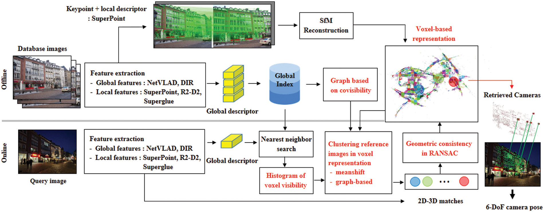
Figure 1: Learning-based hierarchical localization system [14] using proposed method

2  Method

Hierarchical localization methods create global and local descriptors of DB images offline (in the training stage) using a coarse-to-fine approach [14,19]. In the test stage, global and local descriptors are similarly extracted from the query image. First, candidate images (reference views) are determined by searching the DB images globally, which reduces the domain to be matched. Subsequently, the keypoints of the query image and reference views are locally matched. A wrong location hypothesis in global matching significantly affects the performances of hierarchical methods. In this study, the 3D points of the DB images were computed using the SfM methods during training. Therefore, the 2D keypoints detected in the query image were matched to the 3D points associated with the reference views, and the PnP solver was used to estimate the camera pose.

NetVLAD [19], a representative study on place recognition, was used to extract global descriptors from hierarchical localizations. Fig. 2 shows 15 reference views retrieved for a single query image (red bounding box) from the Aachen Day-Night dataset [22] using NetVLAD. The Aachen dataset describes an old city center in Aachen, Germany. It contains 4,328 images of the old city’s weekly database and 824 and 98 queries, respectively, under day and night conditions. This dataset has a large scene space and contains images captured under various conditions (weather, season, and day-night cycles). The global retrieval results show that the reference views captured from different locations and camera viewpoints can be matched. Fig. 2 shows three reference image groups that are marked with red, green, and blue dotted lines. If the query image is matched with the reference images one by one, outlier images captured at a distant location are matched. The visual features of the image are then used in the local matching stage. Here, the number of inliers set (2D-3D correspondences) that satisfy a geometric consistency check within the RANSAC [8,23,24] is examined.

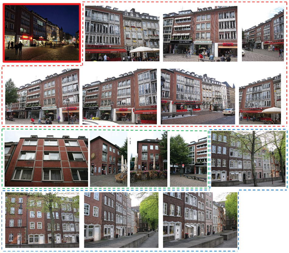
Figure 2: Fifteen matched reference views in the global matching stage. Query image (top left, red box) and reference images (dotted line boxes)

By clustering the reference views with a similar viewpoint, the number of inlier sets in local matching can be increased. In the previous method [14], frames were clustered based on the 3D structures that they co-observed. The connected components (places) were found in a bipartite graph composed of frames and observed 3D points. However, when clustering all images with co-observed 3D points, there are no criteria to measure the degree of covisibility of the 3D points. If a video sequence with many successive frames is used as the training dataset, regions that are too large to include common visual features may be clustered in the same places. To address this, this paper introduces two methods for the covisibility-based clustering of images with similar viewpoints using voxel-based scene representation.

2.1 Voxel-based Scene Representation

The 2D-3D benchmark dataset for camera localization includes 3D points reconstructed using SfM methods such as COLMAP [25,26] and Bundler [27]. In the Aachen dataset, the scale-invariant feature transform (SIFT) and COLMAP are used for image feature matching and 3D reconstruction [22]. Figs. 3a and 3b show that 3D points are mainly distributed in specific regions with many visual features, and many outliers by false matching (with SIFT) are included in the dataset.

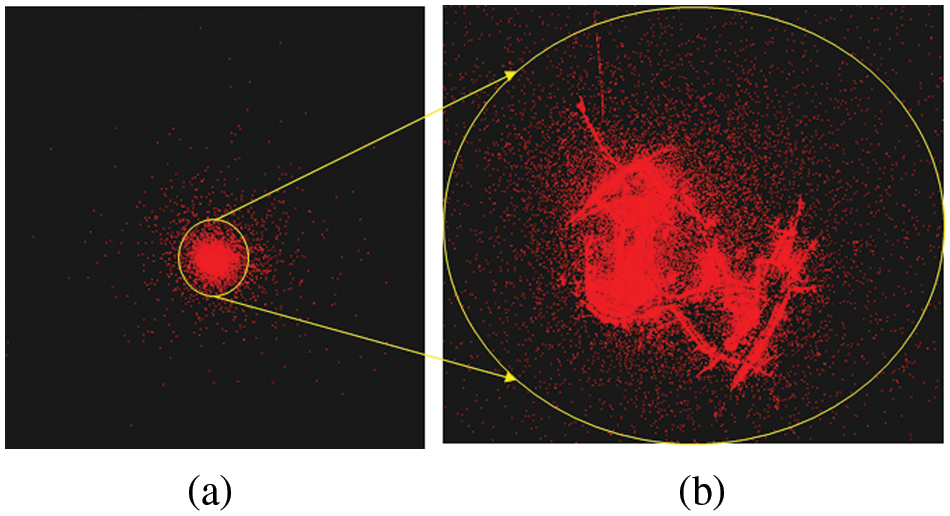
Figure 3: 3D points reconstructed by SIFT in Aachen dataset (a) and their enlarged version (b)

To effectively identify the specific places in the scene space, the scene is represented as a regular tessellation of cubes in Euclidean 3D space [21]. Each voxel was assigned a unique identification number based on its global location. Outliers, such as noisy 3D points, that are very distant from the cloud distribution of 3D points in the scene are removed first. Then, the number and size of voxels are determined based on the scene volume and the number of 3D points. False matches among 2D-3D correspondences can be identified and removed by examining whether the voxel regions detected in an input image maintain geometric consistency (such as left–right order).

In our previous voxel-based representation [21], RANSAC-based plane fitting was applied to the 3D points in a voxel to obtain the main plane in which the inlier points on the main plane were determined. Because the exterior walls of a building, the ground, and the outer surface of an object are captured using a camera, outdoor scenes with many manufactured structures can be approximated using major planes. In addition, points that are distributed on the main plane are more likely to be captured from multiple viewpoints by the camera. This is because the points occluded on a surface with respect to a given viewpoint increase as the surface’s geometric complexity increases. In some cases, the main planes correspond to the exterior walls and ground. However, when there are several objects such as streetlights and trees in the scene, an unexpected plane that is entirely different from the original scene structure is often obtained. Therefore, to solve this problem, the RANSAC-based plane-fitting procedure and the centroid of the main plane were excluded.

It is essential to detect rich and widespread feature sets over the entire scene space for precise scene description and matching. In visual feature (corner point) detection and matching, SuperPoint [28] is used to detect and precisely match a set of evenly distributed points of interest. Fig. 4a shows the feature points detected and matched using SuperPoint. As a result, a considerable number of outliers and noisy 3D points were removed. Fig. 5 shows the process of defining the voxel volume and identifying the 3D points in each voxel. First, the maximum and minimum coordinate values of the x-, y-, and z-axes of the 3D points were found, and the voxel width, length, and height were computed. The number and size of the voxels were determined according to the scene volume and the number of 3D points. Second, the number of points within each voxel was counted. If this value was below a specific threshold, the voxel was considered an outlier and removed. Finally, the remaining voxels and their 3D points were indexed and labeled. Fig. 4b shows the distribution of 3D points in the proposed voxel representation, each marked with different colors.

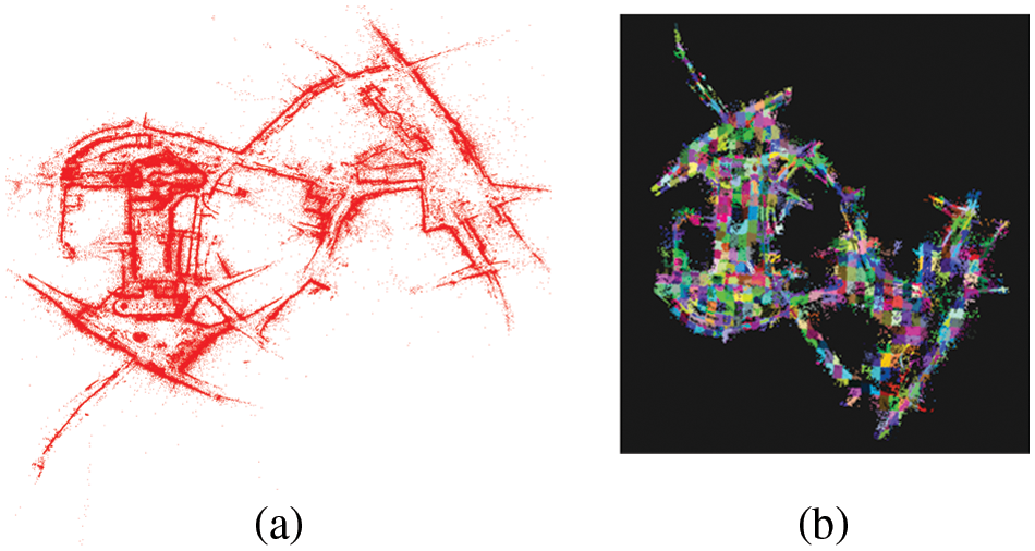
Figure 4: 3D points by SuperPoint [28] and COLMAP [25] (a) and voxel-based representation (b)

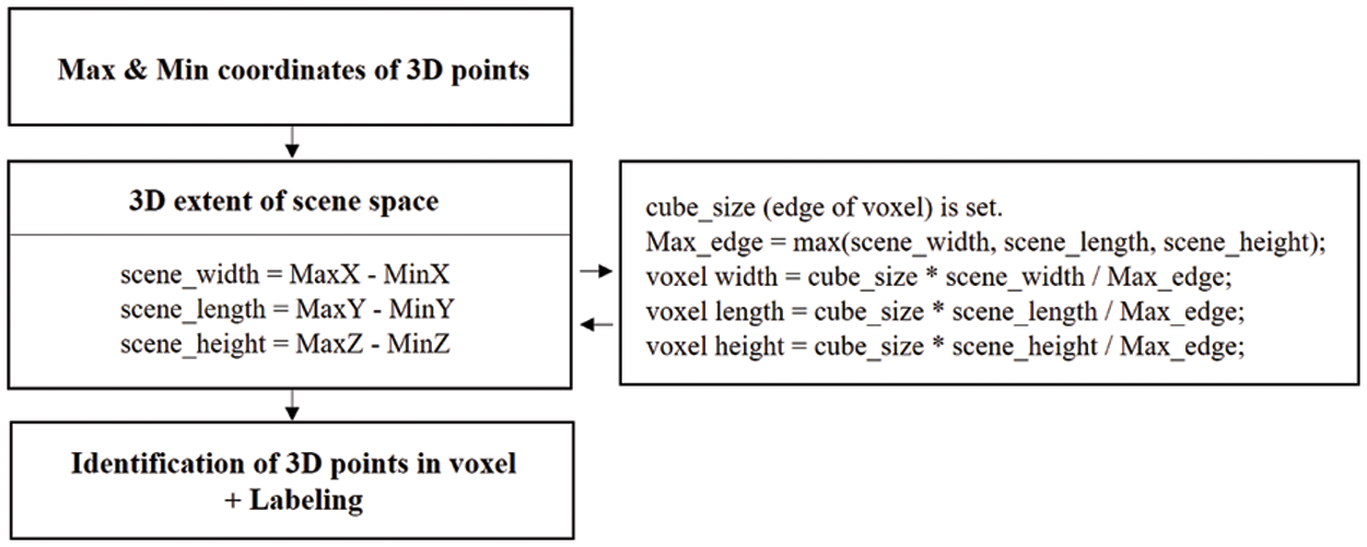
Figure 5: Determining voxel volume and labeling 3D points

2.2 Reference Image Clustering Based on Covisibility

2.2.1 Histogram of Voxel Visibility and Meanshift

In previous hierarchical methods [14,19], common visual clues have been employed in location-based image clustering. This has been very helpful for camera localization. More specifically, images are clustered based on co-observed 3D scene structures, meaning that images correspond to the same place if the same 3D points are visible in them. Therefore, connected components are found in the covisibility graph that links the DB images to 3D points in the model [14]. Thus, these images are likely to be retrieved together using a hierarchical method, which uses 3D points and their visual features. However, because there are many 3D points in a large-scale scene, efficient clustering of 3D points and their visual features in the scene’s location is required. Given the reference images obtained by the global retrieval of a query image, this paper introduced a method to create image clusters with similar viewpoints in the proposed voxel-based scene representation. In this study, the scene was represented with voxels, in which 3D points reconstructed using SfM were indexed. A voxel identification number was assigned to each 3D point. The geometric information was placed in a list structure.

A histogram (Fig. 6) representing the distribution of visible voxels from the reference images was created using global retrieval. In Fig. 6, the x-axis represents the voxel index in the scene space, and the y-axis represents the frequency of voxel visibility in the reference images. Because the visual features and their 3D points in the Aachen dataset were stored, the visible voxels where 3D points were captured could be identified. If a voxel has a higher frequency in the histogram, it is visible in more images. The visibility frequencies of the voxels in the histogram were then sorted in descending order. From the histogram of voxel visibility, K reference images were used to create the cluster set of reference images with similar viewpoints. Fig. 2 shows the query image and its 15 retrieved reference images in the global matching procedure. Some images had the same location as that of the query image, but there were also other images from different locations.

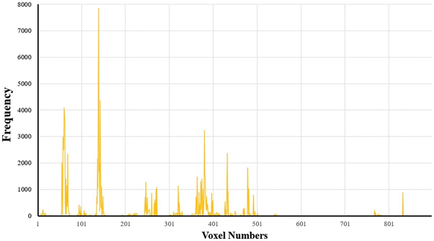
Figure 6: Histogram of voxel visibility

To consider the spatial proximity of neighboring voxels in the voxel clustering procedure, the meanshift method with kernel density estimation [29] was employed. In Eq. (1), for n data points xi, i = 1, …, n in 3D space, the Parzen kernel density estimator fh(x) at point x is given by:

fh(x)=1n∑i=1nKh(x−xi)=1nh∑i=1nK(x−xih),(1)

where Kh(x) is the kernel for the density estimation and its bandwidth parameter h, which determines the considered range of the neighboring voxels.

Because a camera generally has a limited field of view, reference images with similar viewpoints and camera locations share many visual features within the same scene area. Therefore, this paper can create image clusters with similar viewpoints by using the 3D reconstructed points of the reference images. The 20 most re-occurring voxels from the voxel visibility histogram of the query image’s reference images (Fig. 7) were considered. The center coordinates of the voxels were weighted in proportion to the visibility frequencies of the bins. Fig. 7a shows the center coordinates of the 20 voxels, from blue to red (most to least common). In 3D space, the meanshift method based on the K-nearest neighbor (K-NN) rule was employed instead of the Parzen kernel density estimator because it is faster and allows for higher dimensions. Fig. 7b shows the cluster areas (colored regions) and their center positions (‘X’) using meanshift. The obtained clusters were used for camera pose estimation using 2D-3D correspondence with local descriptor information.

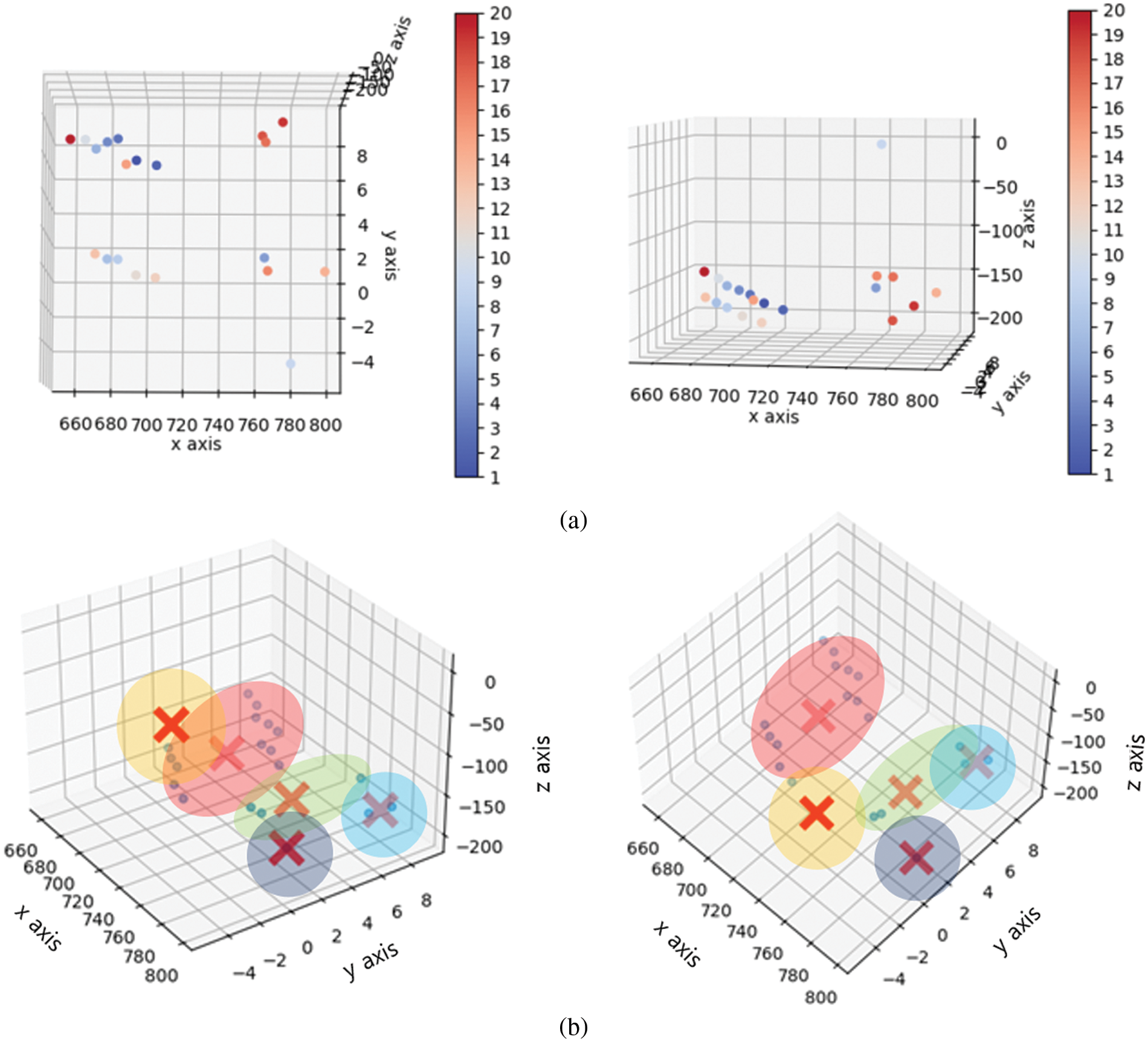
Figure 7: (a) Center points of 20 voxels in the order of their visibility frequency and (b) their corresponding cluster regions and center positions (marked with ‘X’), generated using the meanshift algorithm

2.2.2 Graph Clustering Based on Voxel Covisibility

Meanshift clustering requires the bandwidth parameter h of the kernel function (see Eq. (1)) or the bandwidth to include K-nearest neighbors, which in turn affects the results of meanshift clustering using the spatial proximity of voxels. Because local areas generally have a variety of structures in a large-scale scene, it is difficult to determine the optimal bandwidth parameter in the meanshift clustering process. Furthermore, the bandwidth parameter significantly affects the processing time because more data is required as the bandwidth radius increases.

For efficient clustering of the reference images of the query, this paper introduces a graph structure for the covisibility relationship of voxels. The nodes of the graph were the voxels in the scene, and the eight voxels adjacent to each voxel were considered the neighborhood. The edges of the graph were weighted based on the relative covisibility of the adjacent voxels. In the proposed graph representation, the cost values of the adjacency matrix were based on each voxel’s covisible voxels. The proposed method stored the index information of voxels visible in DB images as a data structure, which was used to obtain the number of covisible voxels for each voxel (see Fig. 8a). For example, the first voxel (Voxel 1) was visible in 31 training images. When Voxel 2 appeared in seven images that voxel 1 was visible in and had a higher covisibility with Voxel 1 than the other voxels. The relative covisibility was computed by dividing the covisibility frequencies of the neighboring voxels by the number of times the voxel of interest is visible. In Fig. 8a, the covisibility ratio of Voxel 2 relative to Voxel 1 is 0.2258. For each voxel, the average covisibility ratios of the adjacent voxels were computed according to the level of the graph. The covisibility ratio at each graph level depends on the local complexity of the scene. The more complex the scene structure, the lower the covisibility ratio at a given graph level. In addition, as shown in Fig. 8b, the average covisibility ratios decrease as the scene structure complexity increases because cameras generally have a limited field of view. The average ratios in the graph levels were used to determine the number of adjacent nodes considered in the clustering procedure. Subsequently, by applying the breadth-first search method to the graph, the connected components (adjacent voxels) of the voxel of interest were examined, as shown in Fig. 9a. More specifically, when the average covisibility of the adjacent voxel was higher than that of all voxels at each depth level, it was determined that the voxels were connected to the voxel of interest. Fig. 9b shows the graph structure of Voxel 1, which has edges with higher covisibility values than the average values of other voxels at each level. Here the colors of the nodes (yellow, green, blue, purple, and pale blue) represent the connectivity of Voxel 1 as the level of the graph increases. Voxels that appear concurrently in DB images can be clustered using this procedure, and this is utilized in the preprocessing steps.

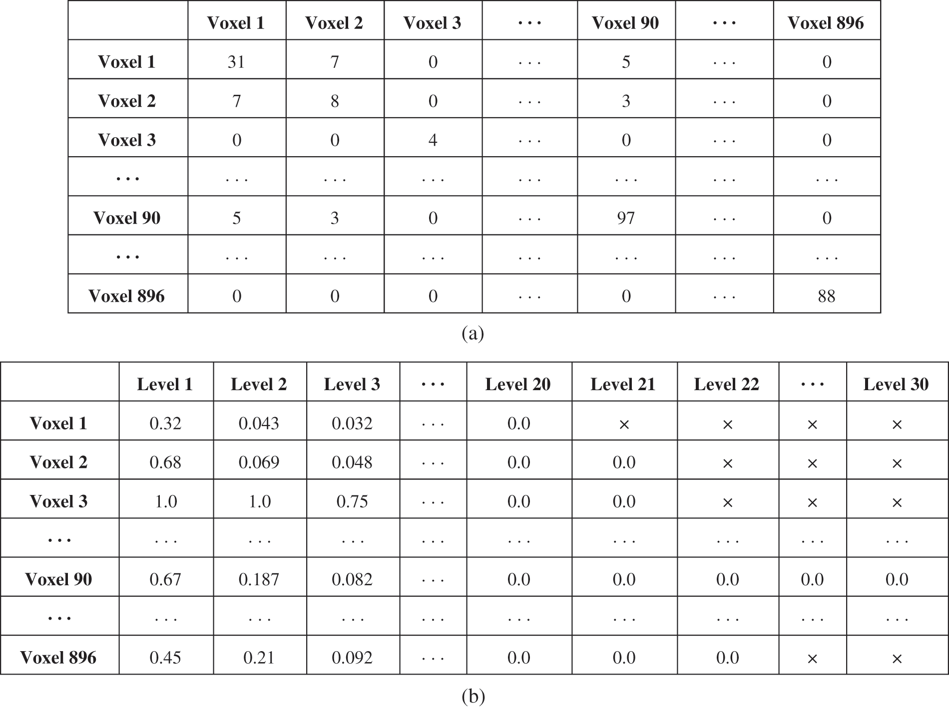
Figure 8: Number of voxels that are covisible for each voxel (a) and average covisibility values at each graph depth level (b)

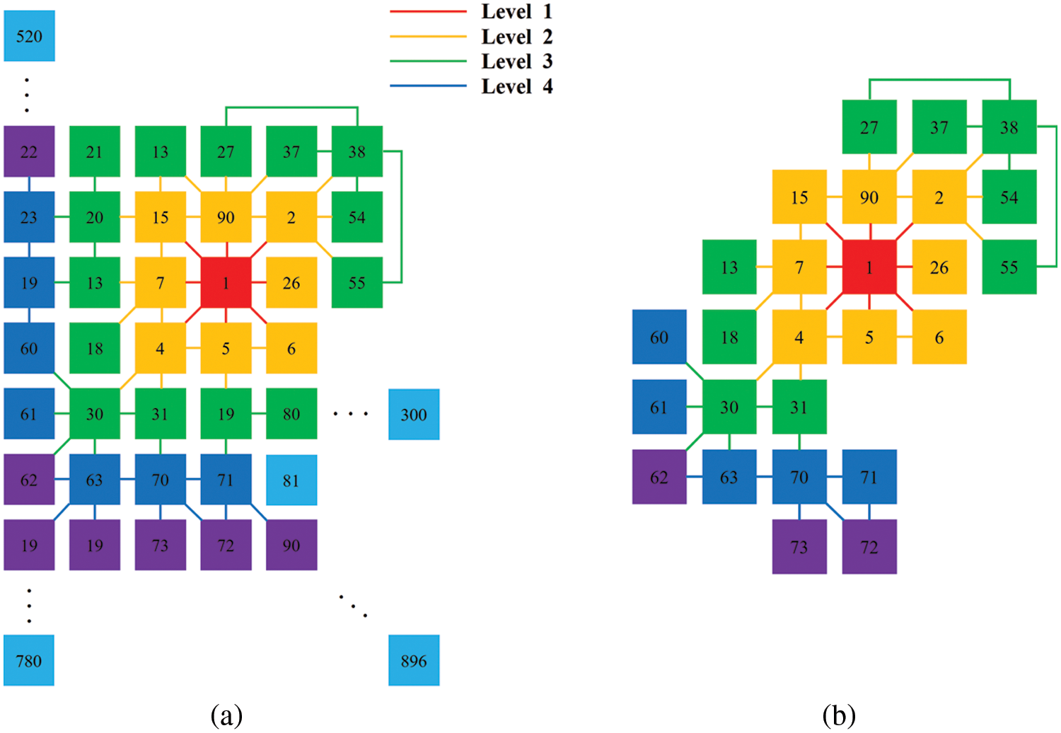
Figure 9: Adjacent voxels for voxel 1(a) and voxels with high covisibility ratios (b)

In the global matching procedure, a query’s reference images were retrieved along with their corresponding voxel index information. The highest-ranked T voxels in the visibility histogram generated from reference images were then found. Voxel clusters with a high visual coherence were generated using the graph structures of the T voxels. Therefore, visible voxels (covisible scene areas) could be determined simultaneously when T voxels were captured. In this clustering procedure, the lowest-ranked voxel of T voxels was added to the highest-ranked voxel if these two voxels were found to be spatially connected. If two voxels were found not to be connected, a different voxel cluster was generated. The identification information of the voxels appearing in the reference images was compared with that of the voxel clusters. When more than half the voxels in a reference image were found to be in a specific voxel cluster, the reference image was considered to be part of that voxel cluster. In this procedure, M reference images were grouped into N reference image groups (M ≫ N). The final reference image group was used in local descriptor matching, in which local descriptor information was collected for each group. The reference image groups were generated by checking the connection elements of the voxel graph of the ranked voxels.

In the proposed voxel-based representation, the visibility of every voxel (V) in a scene is 0 considered. Therefore, the space complexity of generating the voxel-based histogram is O(V). Consider that M reference images are retrieved by global matching, and the number of 3D points in the M-th reference image is pM. The total number of 3D points present in M reference images is a summation of all (pM) values. The time (computation) complexity of generating the voxel-based histogram is, therefore, O(sum(pM)). The time complexity of the meanshift is expressed as O(T2), where T is the number of data samples. In the proposed method, T is the number of the most highly re-occurring voxels in the query image’s reference images according to the voxel visibility histogram. Its space complexity is O(T). In graph-based clustering, we examined how often each voxel appears in the same reference image as every other voxel, as shown in Fig. 8a. In computing the covisibility of V voxels, the time and space complexity are both O(V2). For each voxel, the average covisibility values were computed at each graph depth level d as shown in Fig. 8b. Since this processing is performed for V voxels, the time complexity is O(Vd). The connected components (adjacent voxels) of the voxel of interest that have more than the average covisibility, were examined by applying the breadth-first search to the graph structure. The breadth-first search’s time and space complexity are O(V). In our graph-based clustering, the total time complexity is O(V2) + O(Vd) + O(V) ≒ O(V2) and the space complexity is O(V2) + O(V2) + O(V) ≒ O(V2). After the above-mentioned pre-processing, voxel clusters are finally generated. The most highly re-occurring voxels T are chosen using the voxel-based histogram. Pre-built voxel clusters to identify low-ranked voxel clusters that may be connected to higher-ranked voxel clusters were then examined. The time complexity of this inference is O(T2), and its space complexity is O(T). The voxel graph-based method has less computational load than the meanshift method because the covisibility graph of voxels is pre-built from the DB images. In addition, this method does not require the bandwidth parameter of the meanshift to be set.

The reference images were mapped to each location in these procedures, and each cluster was then matched independently to the 2D keypoints detected in the query image. To estimate the camera pose, a local description was extracted from the query and reference images. Because the 3D points of the feature points in the reference images were already in the data structure, a 2D-3D correspondence from the local matching could be established. PnP is employed to estimate the pose of a calibrated camera, which minimizes reprojection error (the sum of squared distances between the image points and the projected 3D points). Here the PnP-based geometric consistency within the RANSAC scheme was checked. This PnP-based geometric consistency within the RANSAC scheme makes the final pose more robust to outliers (false 2D-3D correspondences). The ratio of the number of inlier points to that of all the feature points in the reference image was computed. The PnP result supported by the most inlier points was regarded as the final camera pose. The camera pose with 6 degree of freedom represents the rotational direction with respect to pitch, yaw, and roll, and the position in the X-, Y-, and Z-axes.

2.3 Hierarchical Method Implementation

Learning-based hierarchical localization methods are comprised of global and local description extractors along with their matching procedures. In this study, SuperPoint [28], R2-D2 [30], and Superglue [31] were used as local descriptors, and NetVLAD [19] and DIR [32] were used as global descriptors. The input was a grayscale image with a maximum resolution of 1024 pixels vertically or horizontally. The dimensions of the global descriptors were reduced to 1024. The weights of NetVLAD and DIR were learned using the Pitts-30k and Google-landmarks datasets, respectively. In both SuperPoint and R2-D2 methods, a non-maximum-suppression method was employed to avoid obtaining too many feature points from the query image. The suppression radius for each feature point was set to 3 pixels. The weights of SuperPoint, R2-D2, and Superglue were learned using the MS-COCO 2014, Aachen, and MegaDepth datasets, respectively.

3  Experimental Results

Reference images were attained using global retrieval and a histogram representing the distribution of visible voxels generated. T highly ranked voxels were then selected from the histogram. After the reference images were clustered based on the T-most highly ranked voxels, the query image and reference image clusters were locally matched, 2D-3D correspondence established, and camera pose estimated. In this experiment, T was set as 20, 50, and 100.

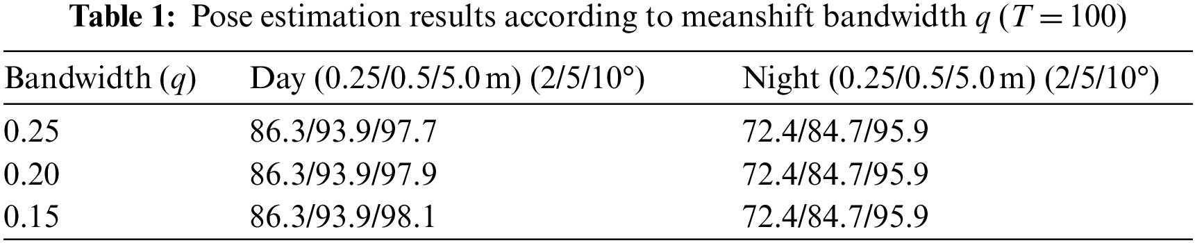
In the meanshift method, clustering results are affected by the bandwidth parameter. Here, the bandwidth of the meanshift was determined using the K-NN technique. When the total number of 3D points and the estimation parameter q were 100 and 0.3, respectively, the meanshift continued to expand the interest region until 30 points were included. Therefore, the bandwidth was determined based on the average distance between 3D points within the same cluster. Table 1 shows the accuracy according to bandwidth q of the meanshift when 100 voxels are considered. The percentage of query images (824 and 98 queries under day and night conditions, respectively) localized within X m and Y° of their ground-truth pose was measured [13]. In all conditions and times, three pose accuracy intervals were defined by varying the thresholds: high precision (0.25 m, 2°), medium precision (0.5 m, 5°), and coarse precision (5 m, 10°). Table 1 shows that there were few differences in performance when sufficient voxels (T = 100) were chosen from the visibility histogram. The best performance was obtained in the case when q = 0.15.

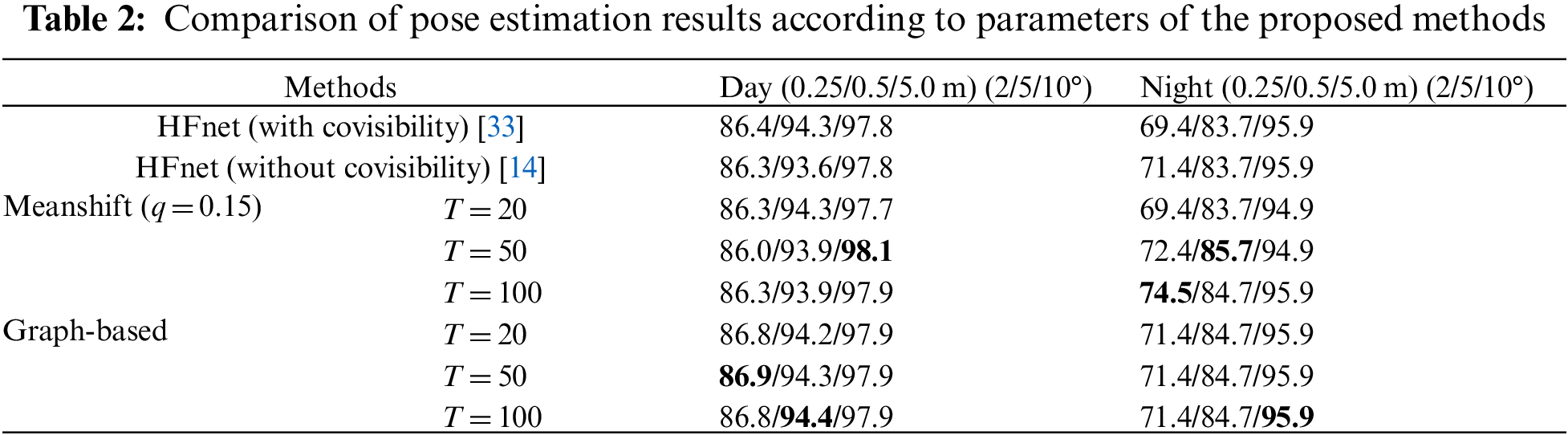
In Table 2, previous methods [14,33] are compared with the proposed methods regarding parameters T and q. The first method (HFnet with covisibility) determines the connected components in a bipartite graph composed of frames and observed 3D points [14]. Reference images are clustered if they observe some common 3D points. Although the previous method is similar to the proposed method in that prior frames are clustered based on 3D structure covisibility, no schematic clustering method is described. For example, too many or too few clusters may be generated because only the covisibility of 3D points is considered; therefore, the obtained reference image clusters are significantly affected by the complexity of the scene structure and continuity of the image frames. Here, the local descriptors of the reference images in each cluster were matched with the query image, and the accuracy of the results was computed using the most inlying set in the RANSAC-based PnP pose estimation scheme. The second row of Table 2 shows the results obtained using HFnet [14] without considering covisibility, which were obtained by matching all the local descriptors of 50 reference images. The graph-based method performed slightly better than the meanshift method under daytime conditions; however, under nighttime conditions, the camera estimation results using meanshift were best in most cases. Table 2 shows that the number of reference image clusters affects the performances of the two methods.

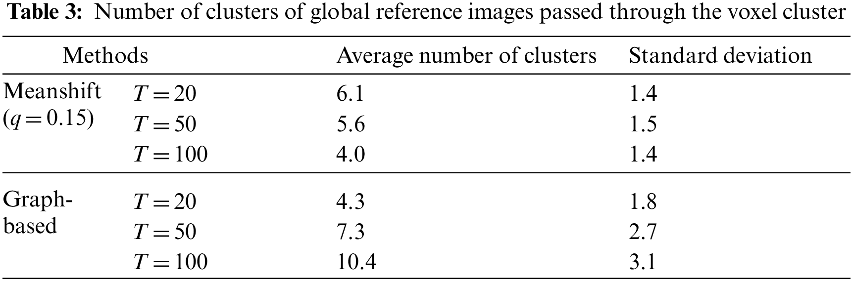
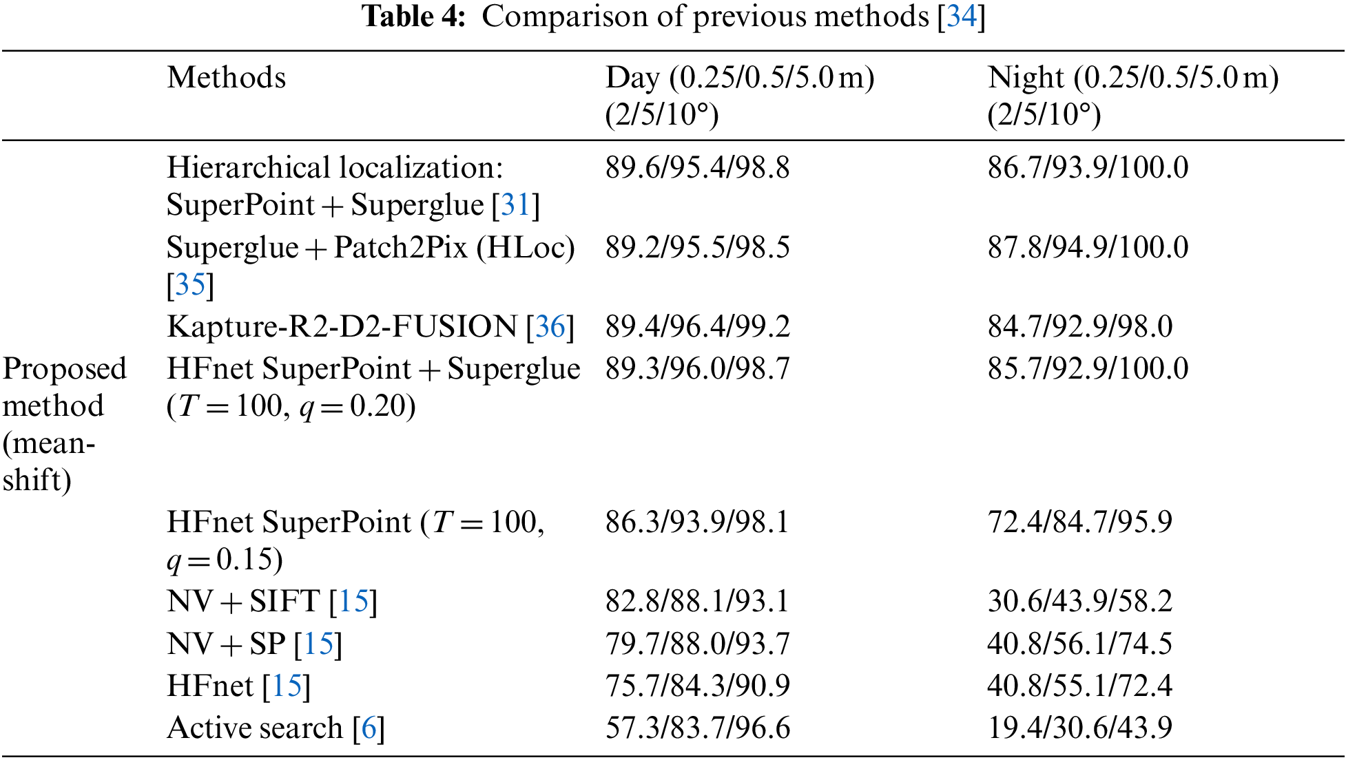
As shown in Table 3, more clusters were generated using the graph-based method than the meanshift method; therefore, the scene structure of the reference images was more refined using the graph-based method. In general, the local matching performance was affected by the significant difference in visual features under night and day conditions. When fewer clusters were generated, each cluster included more reference images and local description information because the number of reference images was fixed at 50. Therefore, when more local descriptions were considered in each local matching, the matching performance by the meanshift method at night was slightly better. In Table 4, the proposed method is compared with previous methods on a benchmark dataset [34]. The pose estimation performance improved when the SuperPoint and Superglue methods were employed.

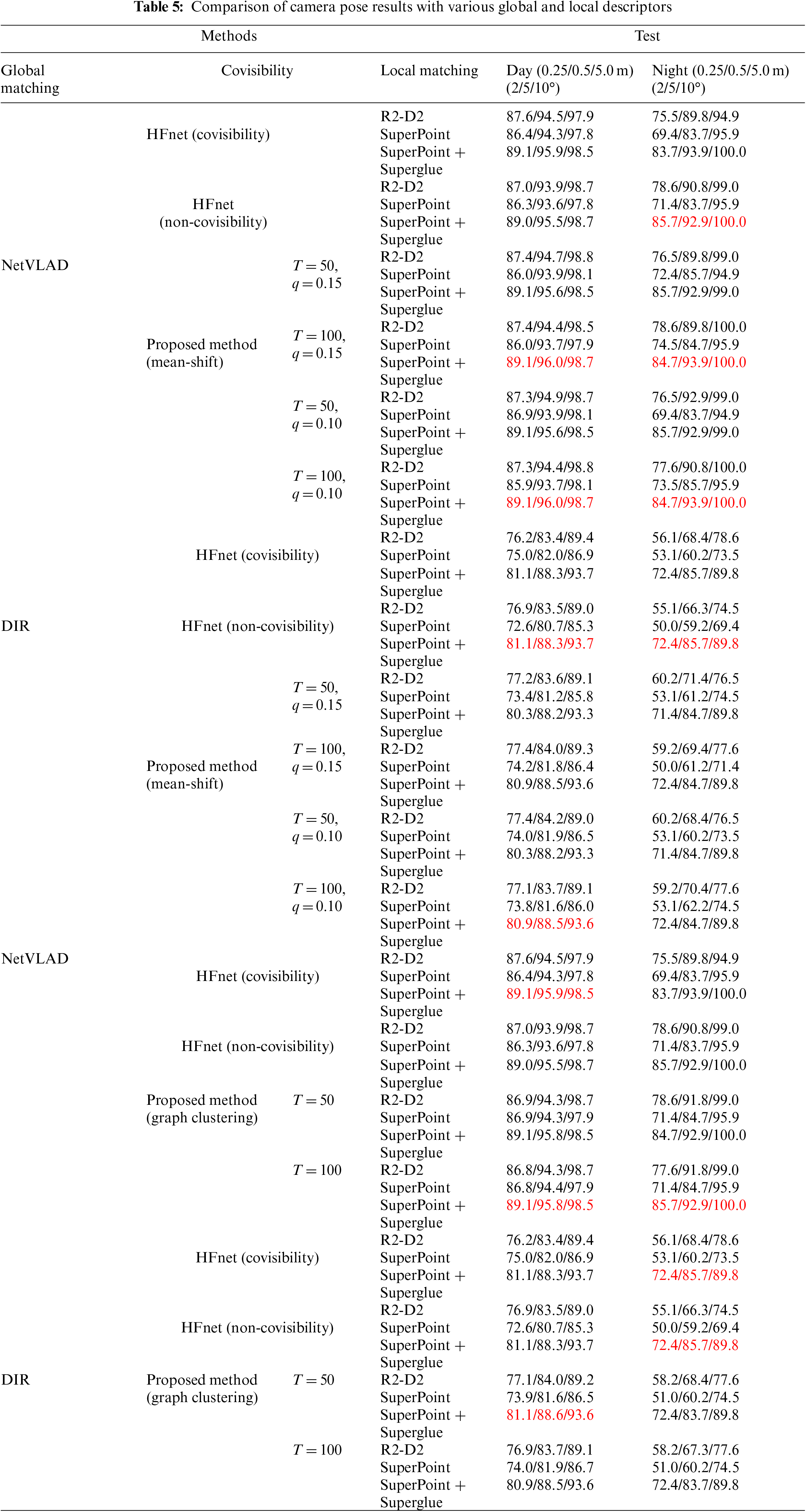
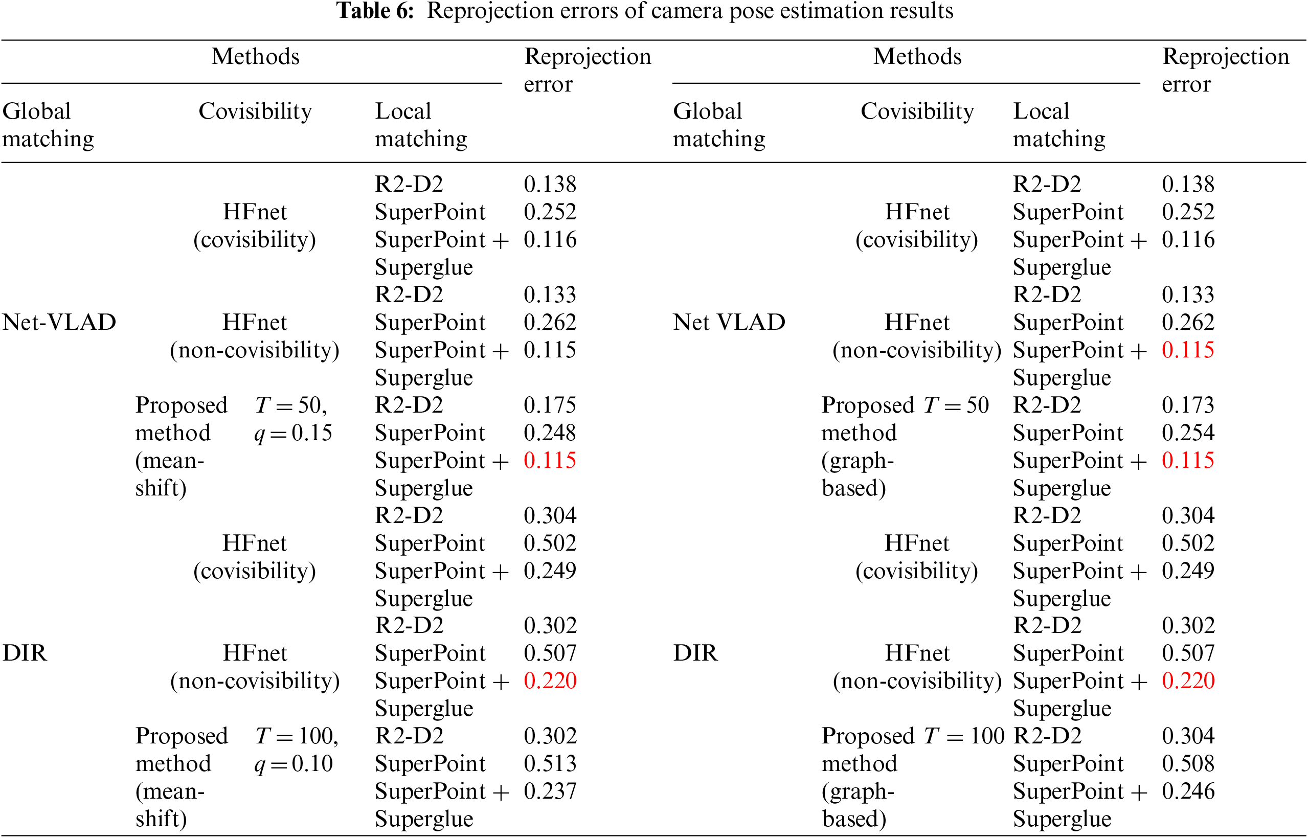
In Table 5, the performance of the proposed method is compared with that of two global descriptors and three regional descriptors in the hierarchical approach. In all cases, NetVLAD yielded better results than DIR. To evaluate the accuracy of the camera pose estimation results, the reprojection error was calculated (Table 6). In Tables 5 and 6, the best results for each case (the global descriptor) are highlighted in red. In the experimental results, the proposed approaches have been compared with state-of-the-art approaches for camera localization, using various parameter configurations.

4  Conclusion

In a large-scale scene, the descriptor space of the visual features becomes quite large, which results in the increase of 2D-3D camera pose estimation matching errors. This paper introduced two clustering methods based on the covisibility of reference images in the hierarchical approach. Because neighboring visual features are captured simultaneously when a camera focuses on the scene location, clustering the reference images extracted via global matching improves the local matching performance. The reference images were clustered according to two criteria: the visibility frequency of visual features and the covisibility of features. Voxel-based scene representation constructed using 2D-3D correspondence enabled us to efficiently identify the areas that were visible most often in the reference images. A histogram representing the distribution of the visible voxels in the reference images was built. The relatively important voxels (such as those that are the most visible in the scene) were then identified in the order of the voxels’ frequency of visibility in the reference images. To consider the distribution of neighboring voxels in the voxel clustering procedure, meanshift and graph-based methods were employed. In the meanshift method, the center coordinates of the voxels were weighted proportionally to the visibility frequencies of the voxels, and a meanshift was applied to the center coordinates of each voxel. In the graph-based method, a graph of the covisibility relationship of voxels from the training images was built. By examining the voxel graph of the highest-ranked voxels in the reference images, reference image groups were generated. The graph-based method had better computational efficiency than the meanshift method because the covisibility graph was built in advance. Because reference images of similar scene locations were clustered, local matching with the query image was easier, and the number of outliers decreased. The experimental results showed that camera pose estimation using the proposed approaches was more accurate than that of previous methods. The proposed clustering methods for reference images are relatively effective in improving performance in large-scale environment.

Funding Statement: This research was supported by the Basic Science Research Program through the National Research Foundation of Korea (NRF) funded by the Ministry of Education (NRF-2018R1D1A1B07049932).

Conflicts of Interest: The authors declare that they have no conflicts of interest to report regarding the present study.

References

1. D. Mahajan, R. Girshick, V. Ramanathan, K. He and M. Paluri et al., “Exploring the limits of weakly supervised pretraining,” in Proc. of the European Conf. on Computer Vision, Munich, Germany, pp. 181–196, 2018. [Google Scholar]

2. M. Tan and Q. V. Le, “EfficientNet: Rethinking model scaling for convolutional neural networks,” arXiv preprint arXiv:1905.11946, 2019. [Google Scholar]

3. C. Szegedy, W. Liu, Y. Jia, P. Sermanet and S. Reed et al., “Going deeper with convolutions,” in Proc. of IEEE Conf. on Computer Vision and Pattern Recognition, Boston, MA, USA, pp. 1–9, 2015. [Google Scholar]

4. N. Westlake, H. Cai and P. Hall, “Detecting people in artwork with cnns,” in Proc. of the European Conf. on Computer Vision, Amsterdam, Netherlands, pp. 825–841, 2016. [Google Scholar]

5. Y. Zhu, K. Sapra, F. A. Reda, K. J. Shih and S. Newsam et al., “Improving semantic segmentation via video propagation and label relaxation,” in Proc. of IEEE Conf. on Computer Vision and Pattern Recognition, Long Beach, CA, USA, pp. 8856–8865, 2019. [Google Scholar]

6. T. Sattler, B. Leibe and L. Kobbelt, “Efficient & effective prioritized matching for large-scale image-based localization,” IEEE Transactions on Pattern Analysis and Machine Intelligence, Mach. Intell., vol. 39, no. 9, pp. 1744–1756, 2016. [Google Scholar]

7. A. J. Davison, I. D. Reid, N. D. Molton and O. Stasse, “MonoSLAM: Real-time single camera slam,” IEEE Transactions on Pattern Analysis and Machine Intelligence, Mach. Intell., vol. 29, no. 6, pp. 1052–1067, 2007. [Google Scholar]

8. M. A. Fischler and R. C. Bolles, “Random sample consensus: A paradigm for model fitting with applications to image analysis and automated cartography,” Communications of the Association for Computing Machinery, vol. 24, no. 6, pp. 381–395, 1981. [Google Scholar]

9. L. Liu, H. Li and Y. Dai, “Efficient global 2d3d matching for camera localization in a large-scale 3d map,” in Proc. of IEEE Int. Conf. on Computer Vision, Venie, Italy, pp. 2372–2381, 2017. [Google Scholar]

10. H. Taira, M. Okutomi, T. Sattler, M. Cimpoi and M. Pollefeys et al., “InLoc: Indoor visual localization with dense matching and view synthesis,” in Proc. IEEE Conf. on Computer Vision and Pattern Recognition, Salt Lake City, UT, USA, pp. 7199–7209, 2018. [Google Scholar]

11. L. Svarm, O. Enqvist, F. Kahl and M. Os-karsson, “City-scale localization for cameras with known vertical direction,” IEEE Transactions on Pattern Analysis and Machine Intelligence, Mach. Intell., vol. 39, no. 7, pp. 1455–1461, 2017. [Google Scholar]

12. C. Toft, E. Stenborg, L. Hammarstrand, L. Brynte and M. Pollefeys et al., “Semantic match consistency for long-term visual localization,” in Proc. of the European Conf. on Computer Vision, Munich, Germany, pp. 383–399, 2018. [Google Scholar]

13. T. Sattler, W. Maddern, C. Toft, A. Torii and L. Hammarstrand et al., “Benchmarking 6DOF outdoor visual localization in changing conditions,” in Proc. of IEEE Conf. on Computer Vision and Pattern Recognition, Salt Lake City, UT, USA, pp. 8601–8610, 2018. [Google Scholar]

14. P. E. Sarlin, C. Cadena, R. Siegwart and M. Dymczyk, “From coarse to fine: Robust hierarchical localization at large scale,” in Proc. of IEEE Conf. on Computer Vision and Pattern Recognition, Long Beach, California, pp. 12716–12725, 2019. [Google Scholar]

15. A. Kenall, M. Grimes and R. Cipolla, “PoseNet: A convolutional network for real-time 6-DOF camera relocalization,” in Proc. of IEEE Int. Conf. on Computer Vision, Santiago, Chile, pp. 2938–2946, 2015. [Google Scholar]

16. N. Radwan, A. Valada and W. Burgard, “VLocNet++: Deep multitask learning for semantic visual localization and odometry,” IEEE Robotics and Automation Letters, vol. 3, pp. 4407–4414, 2018. [Google Scholar]

17. Y. Xiang, T. Schmidt, V. Narayanan and D. Fox, “PoseCNN: A convolutional neural network for 6d object pose estimation in cluttered scenes,” in Proc. of the Robotics: Science and Systems XIV, Pittsburgh, PA, USA, pp. 1–10, 2018. [Google Scholar]

18. T. Sattler, Q. Zhou, M. Pollefeys and L. Leal-Taixe, “Understanding the limitations of cnn-based absolute camera pose regression,” in Proc. of IEEE Conf. on Computer Vision and Pattern Recognition, Long Beach, CA, USA, pp. 3302–3312, 2019. [Google Scholar]

19. R. Arandjelovic, P. Gronat, A. Torii, T. Pajdla and J. Sivic, “NetVLAD: Cnn architecture for weakly supervised place recognition,” in Proc. of IEEE Conf. on Computer Vision and Pattern Recognition, Las Vegas, NV, USA, pp. 5297–5307, 2016. [Google Scholar]

20. H. Jégou, M. Douze, C. Schmid and P. Pérez, “Aggregating local descriptors into a compact image representation,” in Proc. of IEEE Conf. on Computer Vision and Pattern Recognition, San Francisco, CA, USA, pp. 3304–3311, 2010. [Google Scholar]

21. S. Lee, H. Hong and C. Eem, “Voxel-based scene representation for camera pose estimation of a single rgb image,” Applied Sciences, vol. 10, no. 24, pp. 8866, 2020. [Google Scholar]

22. T. Sattler, T. Weyand, B. Leibe and L. Kobbelt, “Image retrieval for image-based localization revisited,” in Proc. of British Machine Vision Conf., Guildford, UK, pp. 76.1–76.12, 2012. [Google Scholar]

23. O. Chum and J. Matas, “Optimal randomized ransac,” IEEE Transactions on Pattern Analysis and Machine Intelligence, Mach. Intell., vol. 30, no. 8, pp. 1472–1482, 2008. [Google Scholar]

24. K. Lebeda, E. Juan, S. Matas and O. Chum, “Fixing the locally optimized ransac,” in Proc. of British Machine Vision Conf., Surrey, UK, pp. 1–11, 2012. [Google Scholar]

25. J. L. Schonberger and J. M. Frahm, “Structure-from-motion revisited,” in Proc. of IEEE Conf. on Computer Vision and Pattern Recognition, Las Vegas, NV, USA, pp. 4104–4113, 2016. [Google Scholar]

26. J. L. Schonberger, E. Zheng, M. Pollefeys and J. M. Frahm, “Pixelwise view selection for unstructured multi-view stereo,” in Proc. of the European Conf. on Computer Vision, Amsterdam, Netherlands, pp. 501–518, 2016. [Google Scholar]

27. N. Snavely, S. M. Seitz and R. Szeliski, “Photo tourism: Exploring photo collections in 3d,” The Association for Computing Machinery Transactions on Graphics, vol. 25, no. 3, pp. 835–846, 2006. [Google Scholar]

28. D. DeTone, T. Malisiewicz and A. Rabinovich, “SuperPoint: Self-supervised interest point detection and description,” in Proc. of IEEE Conf. on Computer Vision and Pattern Recognition Workshops, Salt Lake City, UT, USA, pp. 224–236, 2018. [Google Scholar]

29. D. Comaniciu and P. Meer, “Mean shift: A robust approach toward feature space analysis,” IEEE Transactions on Pattern Analysis and Machine Intelligence, Intell., vol. 24, no. 5, pp. 603–619, 2002. [Google Scholar]

30. J. Revaud, P. Weinzaepfel, C. De Souza, N. Pion and G. Csurka et al., “R2d2: Repeatable and reliable detector and descriptor,” arXiv preprint arXiv:1906.06195, 2019. [Google Scholar]

31. P. E. Sarlin, D. DeTone, T. Malisiewicz and A. Rabinovich, “Superglue: Learning feature matching with graph neural networks,” in Proc. of IEEE Conf. on Computer Vision and Pattern Recognition, Seattle, WA, USA, pp. 4938–4947, 2020. [Google Scholar]

32. J. Revaud, J. Almazan, R. S. Rezende and C. R. D. Souza, “Learning with average precision: Training image retrieval with a listwise loss,” in Proc. of Int. Conf. on Computer Vision, Seoul, South Korea, pp. 5107–5116, 2019. [Google Scholar]

33. P. Sarlin, F. Debraine, M. Dymczyk, R. Siegwart and C. Cadena, “Leveraging deep visual descriptors for hierarchical efficient localization,” in Proc. of the 2nd Conf. on Robot Learning, Zurich, Swizerland, pp. 456–465, 2018. [Google Scholar]

34. L. Hammarstrand, F. Kahl, W. Maddern, T. Pajdla, M. Pollefeys et al., Chalmers University of Technology, Long-Term Visual Localization, Gothenburg, Sweden, 2020. [Online]. Available: https://www.visuallocalization.net/benchmark/ [Google Scholar]

35. Q. Zhou, T. Sattler and L. Leal-Taixe, “Patch2pix: Epipolar-guided pixel-level correspondences,” in Proc. of IEEE Conf. on Computer Vision and Pattern Recognition, Nashville, TN, USA, pp. 4669–4678, 2021. [Google Scholar]

36. M. Humenberger, Y. Cabon, N. Guerin, J. Morat, V. Leroy et al., “Robust image retrieval-based visual localization using kapture,” arXiv preprint arXiv:2007.13867, 2020. [Google Scholar]