Variant Wasserstein Generative Adversarial Network Applied on Low Dose CT Image Denoising

1  Introduction

Deep learning (DL) is a part of machine learning (ML). In recent times, ML/DL has been widely utilized in different research directions [1–4], and has become one of the most powerful tools due to recent advances in computer vision. Although DL has been in use since the 1940s, it has been considered an influential revolution in artificial intelligence (AI) research over the last two decades, due to the increasing growth of big data, new architectures, and Graphical Processing Units (GPUs). Recently, there have been several types of deep learning architectures developed, such as Convolutional Neural Networks (CNN) [5], Auto-Encoder (AE), Deep Stacking Networks (DSN), Recurrent Neural Networks (RNN), Restricted Boltzmann Machine (RBM), Long Short-Term Memory (LSTM), Gated Recurrent Unit (GRU) and Generative Adversarial Network (GAN) [6,7]. GAN is an interesting and significant model that attracts the attention of many researchers. While the generative models were defined in 1990 [7], they became very significant and popular only after Goodfellow’s work in 2014 [6]. Nowadays, GAN has expanded into many research areas with various applications and is used in a wide variety of computer vision applications [8–10], security [11], and data generation [12,13]. GAN also attracted researchers’ interest in medical applications by achieving robust diagnostic performance and good results in disease prediction: denoising [14], reconstruction [15], segmentation [16,17], data simulation, anomaly detection [18,19] and classification [20,21].

Another field that has benefited from the GAN revolution is Medical Imaging (MI), a literature that has witnessed great progress in scientific research, current clinical diagnostics, and AI medical applications. There are different medical image modalities (Computed Tomography (CT), X-rays, Magnetic Resonance Imaging (MRI), Optical Coherence Tomography (OCT), Ultrasound, and Microscopy) that have been applied to see inside the human body. MRI is a powerful imaging technology that provides detailed images produced by powerful magnets and radio waves. CT images develop and use a combination of X-rays to show more details than a standard X-Ray image. OCT plays a significant role in detecting many retinal diseases. Ultrasound is a real-time display and comfort over other technologies [22].

CT imaging has grown significantly in the use of medical science over the past few decades, but one of its drawbacks is the risk of radiation exposure, so the radiation is reduced by using low-level doses. The problem with using low-level doses is that the resultant images have more noise and increased artifacts [23].

This paper proposed three variant WGAN models that correlate with Visual Geometry Group (VGG) loss, Structural Similarity Loss, and Structurally Sensitive Loss (SSL). The VGG [24] is based on the perceptual loss to maintain the style and content of the image after denoising. SSL [25,26] efficiently extracts informative features and structural details. SSIM loss [27] helps the model generate visually artistic images because it works on the visible structures in the image. The proposed denoising models are used to enhance the quality of reconstructed images. This paper also shows how well various models perform on both the GPU and the CPU. Following is the rest of this paper: Section 2 defines the CT image denoising problem and presents WGAN-based models for solving it; Section 3 presents the proposed models; Section 4 describes the experiments and results; and Section 5 shows the conclusions and future work.

2  Background and Related Work

GAN was introduced in 2014 [6]. In GAN training, two networks (generator G and discriminator D) are competing in a min-max game, where each network competes against the other. The generator tries to generate new data instances from random noise that are as close to real data as possible to mislead the discriminator. The discriminator tries to differentiate between the real data and the output of the generator. The GAN game can be described using Eq. (1).

minGmaxDV(D,G)=Ex∼Pr(x) [log D(x)]+Ez∼Pz(z) [log(1+D(G(z)))](1)

where E denotes expectation, x is sampled from the probability of real data (Pdata or Pr), z is the input to the generator sampled from some simple noise distribution Pz, such as the uniform distribution or the spherical Gaussian distribution. The two networks of the generator and the discriminator are trained together in a zero-sum game and are adversarial to motivate each other to improve their functionalities. The D network is trained to categorize the input from x sample as real and approximate D(x) to 1; in contrast, if the input is from z sample (a fake sample), the D network tries to categorize it as a fake and approximates D(G(z)) to 0. The G network tries to produce images that look more realistic to trick the discriminator into classifying G(z) as real and approximate D(G(z)) to 1. The loss function of GAN in Eq. (1) is dependent on both KL divergence and Jensen-Shannon (JS) [6,28]. In the original GAN, JS divergence can compare the two data distributions of the generated and real images and assess the similarity between them. GAN is trained to minimize the loss function with an optimal discriminator which minimizes the JS divergence. If the model distribution Pg and real data distribution Pr are very close, this means that the generator learns optimally, and vice versa. Although the goal of GAN training is to reach Nash equilibrium in the two-players adversarial game [29], it is hard to find it, and the training is unstable. It has been proven that GAN is successful in generating images, but it has some disadvantages: training instabilities, network structures, parameter tuning, vanishing gradient, and mode collapse.

WGAN was presented to solve the problems of traditional GANs training because it can stabilize and enhance the training of GANs [29,30]. In WGAN, the loss function was designed to prevent vanishing gradients. Wasserstein Distance is used for measuring the distance and the divergence between two distributions (real data distribution Pr and generator model distribution Pg); it is also called Earth Mover’s distance short for EM distance [30]. The discriminator network (called critic on WGAN) tries to get the least Wasserstein distance between Pr and Pg, and at the same time minimize the loss function. When the Wasserstein distance is very small, the generator network produces outputs that are very close to the distribution of real images. Finally, the weight clipping has been used in WGAN to enforce a Lipschitz constraint on the critic. Having a clipping parameter that is too small can result in the vanishing gradient problem: in contrast, if the clipping is too large, the training fails to converge. The researchers [30] improved the training by using gradient penalty instead of weight clipping for enforcing the Lipschitz constraint. WGAN with gradient penalty is denoted as (WGAN-GP) and the loss function used in WGAN-GP is shown below:

L=Ex~ ∼ Pg[D( x~ )]− Ex ∼ Pr  [D(x)]+λ Ex^ ∼ Px^[(||∇x^D(x^)||2−1)2](2)

where px^ sampling is defined uniformly along straight lines between pairs of points drawn from the real distribution Pr and the generator distribution Pg. It is reported in [30] that WGAN-GP is more stable in learning than standard WGAN. The goal of image denoising is to get a clean image x from a noisy image y, which is shown by y=x+n, where n indicates the Additive White Gaussian Noise (AWGN). Maintaining clinical details and essential properties of the image (corners, edges, texture, and other sharp structures) is essential. Many methods were proposed for LDCT image denoising, which are divided into three divisions: (1) Sinogram domain filtration [31], (2) iterative reconstruction [32], and (3) image post-processing [33]. The sinogram filtering technique such as Filtered Back Projection (FBP), is applied before image reconstruction to raw or log-transformed data to understand the noise characteristics well, so it is usually more effective than iterative reconstruction, which operates on the reconstructed image. In the iterative reconstruction approach, the objective function was optimized by combining the statistical noise model, prior knowledge from the image domain, and imaging system parameters. Image post-processing directly works on an image to suppress artifacts and decrease LDCT noise in the image domain [23].

In recent years, deep learning techniques have been applied to solve the CT image denoising problems to improve the quality of the image. For example, CNN has been used to reduce the noise in LDCT images [34,35]. Kang et al. [36] used a deep CNN network in the wavelet domain. The wavelet-domain CNN has a great denoising power for LDCT images and can remove noise compared to traditional denoising methods. Chen et al. [23] introduced Residual Encoder-Decoder CNN (RED-CNN), which combined autoencoder, deconvolution network, and shortcut connection; it has a good performance for LDCT denoising problem, Ma et al. [37] proposed a dense residual network with self-calibrated convolution (SCRDN) for LDCT images denoising. All these models aim to minimize the Mean Squared Error (MSE) between the generated image from the model and the Normal Dose CT (NDCT) image. Even though the per-pixel MSE results have high PNSR values, these methods can lose some important structural details due to the over-smoothed edge. Recently GAN and WGAN have been used to tackle the previous denoising problems; they were used for enhancing, denoising, deblurring, and getting a good-quality LDCT image. Yang et al. [14] presented WGAN-VGG for LDCT denoising, a model with perceptual loss that compares denoised results from a generator with NDCT image in an established feature space. The model can generate images with less noise and high contrast. Yi et al. [38] proposed Sharpness-Aware GAN (SAGAN) which consists of three networks: UNet generator, discriminator, and sharpness detection network. This model also combined the three losses: the adversarial loss, the sharpness loss, and the traditional pixel-wise loss. The generated images from SAGAN visually achieved results that are attractive with enhanced performance in the quantitative evaluation. You et al. [25] used a Structurally sensitive Multi-scale Generative Adversarial Net (SMGAN) which has two loss functions: the adversarial loss function of WGAN-GP and the structurally sensitive loss. The model (SMGAN) produced high-quality images for LDCT denoising compared to WGAN-VGG. Ma et al. [39] adopted noise learning, the Least Squares GAN (LSGAN), structural similarity loss, and L1 loss for LDCT noise reduction. Their model was able to improve the quality of noise-reduced CT images compared to the state-of-the-art methods. Jeon et al. [40] developed the MM-Net, a novel unsupervised denoising method; consisting of two training steps. The first is to predict the noise-suppressed middle frame with neighboring multi-frame input by training the initial denoising network Multi-Scale Attention U-Net (MSAU-Net) in a self-supervised manner. The second is to improve the image quality by training the U-Net-based final denoiser using the pre-trained MSAU-Net in the first training step. Yin et al. [41] proposed improved Cycle-Consistent Adversarial Networks (CycleGAN) for LDCT image denoising that included a perceptual loss, and a generator network based on U-Net, in which the skip connection between the encoder and decoder path has been reconstructed.

3  The Proposed Denoising Model

The denoising process aims to seek a function T that transfers the LDCT image to the NDCT image and is formulated as x=T(z), where z refers to the LDCT image; x refers to the corresponding NDCT image; and (x, z ∈RH×W×D), where W is the width, H refers to the height and D indicates to the depth of the image. According to Eq. (1), we can sample x from NDCT images distribution or the real image distribution Pr, and z from LDCT images distribution or noise image distribution Pz. The goal of the denoising function T is transferring the image samples from Pz to a certain distribution Pg. Pg represents the denoised distribution of the model, where T approximates Pg as close as possible to Pr. The denoising problem was handled by moving the high noise distribution to the low noise distribution. Increasing the radiation dose to get better image reconstruction can lead to genetic disorders and cancer development in the patients. On the other hand, decreasing the radiation dose by shortening the exposure time can raise the noise and artifacts in the reconstructed images, which may limit the signal-to-noise ratio (SNR) and impair diagnostic information [25]. The noise model in x-ray photon measurements is typically represented by combining Gaussian electronic noise and Poisson quantum noise. In contrast, the noise in reconstructed images is complexly modeled and has non-uniform distribution across the entire image. Therefore, there is uncertainty about the correlation between data distributions of NDCT and LDCT images, which makes LDCT images denoising difficult to solve by traditional methods. Deep learning denoising models can adapt to the ambiguity of the noise images by efficiently extracting high-level features [14]. As mentioned above, the mode collapse and training stability have been overcome by WGAN-GP. This study introduced three models based on WGAN and correlated them with different loss functions to decrease noise in LDCT images and retain the essential informative features and structural details.

3.1 Loss Functions

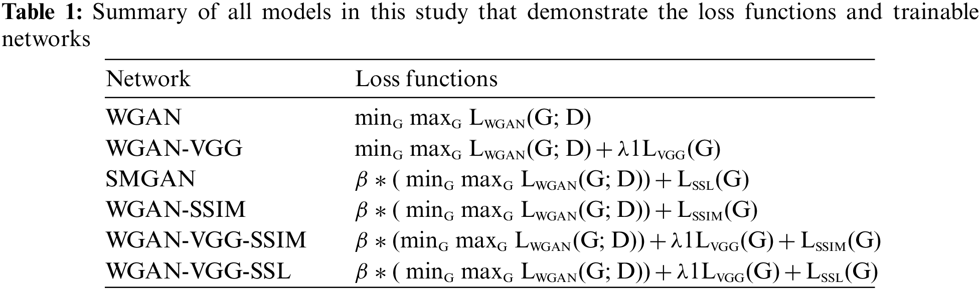
Although the WGAN model solved the vanishing gradient problem, it had many drawbacks. WGAN is hard to train, and it has produced images that have lost many important structural details and edge information. The proposed models handled these problems by employing various loss functions such as VGG loss, SSIM loss, and SSL:

1)   Mean Squared Error (MSE) loss or L2:

It is the normalized Euclidean distance between a denoised patch G(z) from LDCT images and the patch of NDCT images. It is used to minimize the pixel-wise difference between generated images G(z) and the NDCT images. The L2 loss is efficient in reducing the background noise [27]. The formula of L2 loss is shown below:

L2=1HWD||G(z)−x||22(3)

2)   Least Absolute Error (LAE) loss or L1:

It is the absolute distance between the generated image G(z) and the NDCT images. L1 is used to reduce the artifacts. The formula of L1 loss is expressed by Eq. (4):

L1=1HWD|G(z)−x|(4)

3)   Geometry Group (VGG) loss or LVGG:

MSE loss may cause the deformation of details because it blurs the generated images. Thus, the Perceptual Loss (PL) is applied and defined in the feature space rather than directly computing MSE for pixel-to-pixel intensity, as shown in Eq. (5). PL measures the difference in perceptual features between the denoised results from a generator and the real images. It compares high-level perceptual differences like content and style [42].

PL(G)=E(x,z)1HWD||φG(z)−φ(x)||22(5)

where φ is a feature extractor that computes the distance between G(z) and NDCT. A pre-trained VGG-19 network [24] was implemented in this paper as the feature extractor φ. Hence, the perceptual loss can be defined as follows.

LVGG(G)=PL(G)=E(x,z)1HWD||VGG(G(z))−VGG(x)||22(6)

4)   Structural Similarity (SSIM) loss:

It measures the similarity between denoised CT images and NDCT images. The similarity measurement includes three comparisons: contrast, luminance, and structure [27]. SSIM is a visually based metric that performs better than (MSE) in perceptual pattern recognition. The original SSIM is defined as follows.

 SSIM(x,y)=2µxµy+C1µx2µy2+C1∗2σxy+C2σx 2+σy2+C2=L(x,y)∗cs(x,y)(7)

where  μx, µy, σx, σy, and σxy stand for the means, standard deviations, and the cross-covariance of the two images (y,x) from G and the corresponding NDCT image respectively, and C1, C2 are constants [25]. The value of SSIM is close to 1 when x and y are very similar.

 LSSIM=1−SSIM (x,y)(8)

5)   Structurally Sensitive Loss (SSL):

It combines both SSIM loss and L1 loss as in Eq. (9)

LSSL=τ×LSSIM+(1−τ)×L1(9)

Finally, the overall objective functions of all different trained models were expressed in Table. 1.

3.2 Network Structure

A study in [14] was the inspiration for the generator and discriminator network structures.

1.    The generator contains eight convolutional (Conv) layers, and each convolutional layer uses small 3 × 3 kernels. The first seven hidden layers of the G network have 32 filters. In the last layer, only one feature map is generated with a single 3 × 3 filter, which is also the output of the generator network. And the activation function Rectified Linear Unit (ReLU) [43] was used.

2.    The discriminator has six convolutional layers with 64, 64, 128, 128, 256, and 256 filters. Each convolutional layer in the D network has a kernel size of 3 × 3. Then followed by two Fully Connected (FC) layers; the first has 1024 outputs, and the second produces one feature map. Each one is followed by a leaky ReLu, and there is no sigmoid cross entropy layer at the end of the D network. The overall structure of the proposed models is shown in Fig. 1.

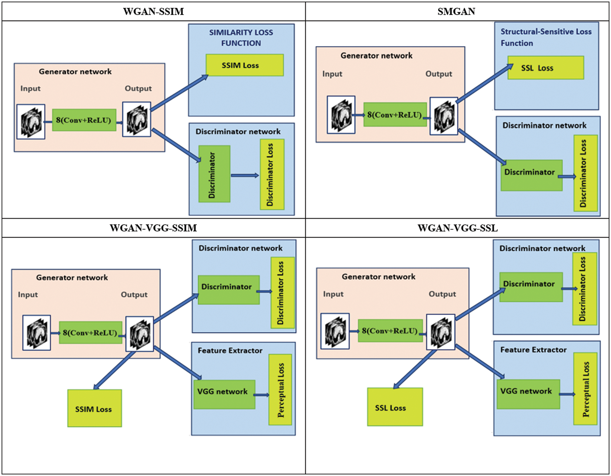
Figure 1: The overall structures of the proposed models

4  Experimental Results

The dataset was used in this paper is a real clinical dataset from Mayo Clinic in the Challenge of 2016 NIH-AAPM-Mayo Clinic Low Dose CT Grand [44], which consists of 10 anonymous patients, divided into seven folders. Each folder contains images of normal-dose abdominal CTs and images of imitated quarter-dose CTs. The folders ‘L067’, ‘L109’, ‘L143’, ‘L291’, ‘L310’, ‘L333’, and ‘L506’ were used for training, and the folders ‘L067’ and ‘L506’ were used for testing. All the networks in this study were implemented in a Python (Python3.6) environment with a PyTorch framework. To differentiate the presented models. The experiments were run on two different devices: a CPU computer with Intel (R) Core (TM) i7-7700HQ CPU @2.8 GHz, 16 GB of RAM, and a NVIDIA GEFORCE GTX 1050. And the second is a GPU computer with Intel (R) Core (TM) i7-7700 CPU @3.60 GHz, 16 GB of RAM, and a NVIDIA Titan XP device.

4.1 Parameter Setting

Both generator and discriminator networks were optimized by utilizing the Adaptive Momentum Estimation (Adam) algorithm [45]. The batch size was 64, and the leaning rate α = 0.0001 according to experiment results (for more detailed information see the supplementary data). β1 = 0.5, β2 = 0.9, and λ = 10 for the balance between the Wasserstein distance and the gradient penalty as suggested in [30], λ1 = 0.1 according to [14], the values of β were set to 0.01 according to our experimental experience. Finally, the parameter τ was equal to 0.1 on the CPU and GPU. The mini-batch size was 128 on the GPU and 80 on the CPU.

4.2 Qualitative Analysis for the Performance of CPU and GPU

4.2.1 Performance of the CPU

To assess the efficiency of the variant loss function, this work trained the proposed models (WGAN-SSIM, WGAN-VGG-SSIM, WGAN-VGG-SSL), and also trained the best-known models such as WGAN [30], WGAN-VGG [14], and SMGAN [25]. We used two examples of a CT image that were taken from the testing data folders ‘L067’ and ‘L506’, and took a zoomed representative slice of each example to show more structure details as a yellow rectangle in Figs. 2 and 3, and Figs. 6 and 7 respectively. The experimental results showed that generated images using WGAN have a more blurred appearance than the other models. Even though WGAN reduced the white artifact, the produced images are not considerably enhanced compared to NDCT images; some structures are over-smoothed, as shown in Fig. 7C with a red arrow. WGAN cannot preserve the edge details as shown in Figs. 2C and 3C, in which generated images lost the textures of the liver. WGAN-VGG has a few white structures. Although it produced images that were sharper than WGAN, it distorted some of the fine structure details. WGAN-VGG has low contrast as shown in Figs. 2D, 3D, and 7D with a yellow arrow; the performance of WGAN has not improved because it just moves from the noise distribution to the free distribution and does not depend on any human perceptual knowledge. On the other hand, perceptual loss is included in WGAN-VGG. WGAN-SSIM achieved visually better than WGAN and WGAN-VGG and preserved features as marked by the yellow arrow in Figs. 6E and 7E. It is noticed that the three models (WGAN-VGG-SSL, SMGAN, and WGAN-VGG-SSIM) preserved the fine image and retained informative details as shown in Figs. 6F–6H, and 7F–7H by red and yellow arrows. Finally, WGAN-VGG-SSL suppressed noise and artifacts, and generated images that are close to NDCT images; it also kept the structural features better than the other methods and determined the lesion location as pointed out by the red dashed circle in Fig. 6H. In conclusion, WGAN-VGG-SSL achieved better informative feature preservations and visual quality than other WGAN methods.

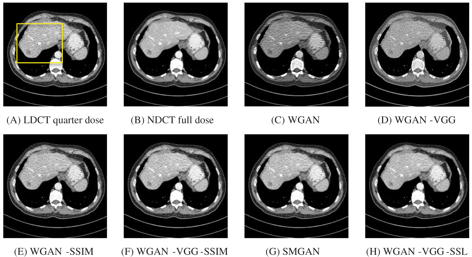
Figure 2: The generated images from the testing data ‘L067’ on CPU at 2000 iterations

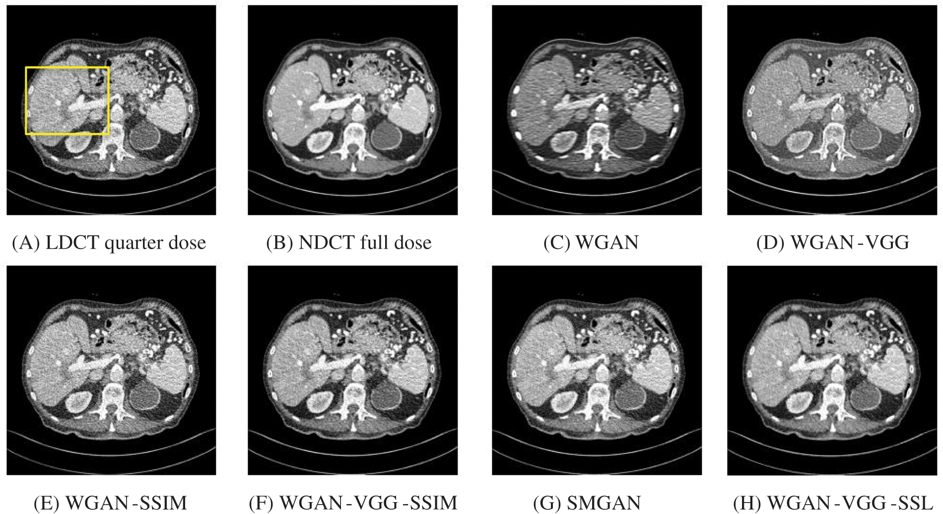
Figure 3: The generated images from the testing data ‘L506’ on CPU at 2000 iterations

4.2.2 Performance of GPU

The time taken on the GPU was 20 times less than that on the CPU. The results of the experiment were taken on GPU after one hour of training. We used two examples of a CT image that were taken from the testing data folders ‘L067’ and ‘L506’, and took a zoomed representative slice of each example to show more structure details as a yellow rectangle in Figs. 4 and 5, and Figs. 8 and 9 respectively. At the beginning of learning, the WGAN model visually had poor informative structures and lost some details about the image, and the generated images were distorted with low contrast. That’s because of the very short training time. The resulting image using the WGAN-VGG preserved some of its characteristics, lost some other details, reduced contrast, and removed the streak artifacts better than WGAN as shown in Figs. 4D, 5D, and 8D by red and yellow arrows. The generated images from WGAN-SSIM preserved some informative details, but they still suffer from white structures. The generated images of WGAN-VGG-SSIM, SMGAN, and WGAN-VGG-SSL preserved more informative features as shown in Figs. 8F–8H, and 9F–9H by red and yellow arrows. They also kept the structural features better than the other methods and determined the lesion location as pointed out by the red circle in Figs. 8F–8H. WGAN-VGG-SSL reduced white structures and artifacts better than SMGAN and WGAN-VGG-SSIM; and produced images similar to NDCT images. The reason why WGAN-VGG-SSL achieved better informative feature preservations and visual quality than other WGAN methods, is that WGAN-VGG-SSL can balance between LSSIM and L1 loss by the weighting factor τ in addition to the VGG loss, as shown in Eq. (9). WGAN-VGG-SSL demonstrated significant quantitative and qualitative results; and has high-level image quality compared with the other denoising models because SSL loss is embedded in WGAN-VGG-SSL. In order to obtain better visual image quality, the models based on SSIM and VGG loss seem to be more desirable for capturing more details and reducing artifacts. SSL presented an informative advantage between adjacent inter-slices. SSIM loss achieved high PNSR and SSIM values, removed complex noise, and helped to stabilize the models.

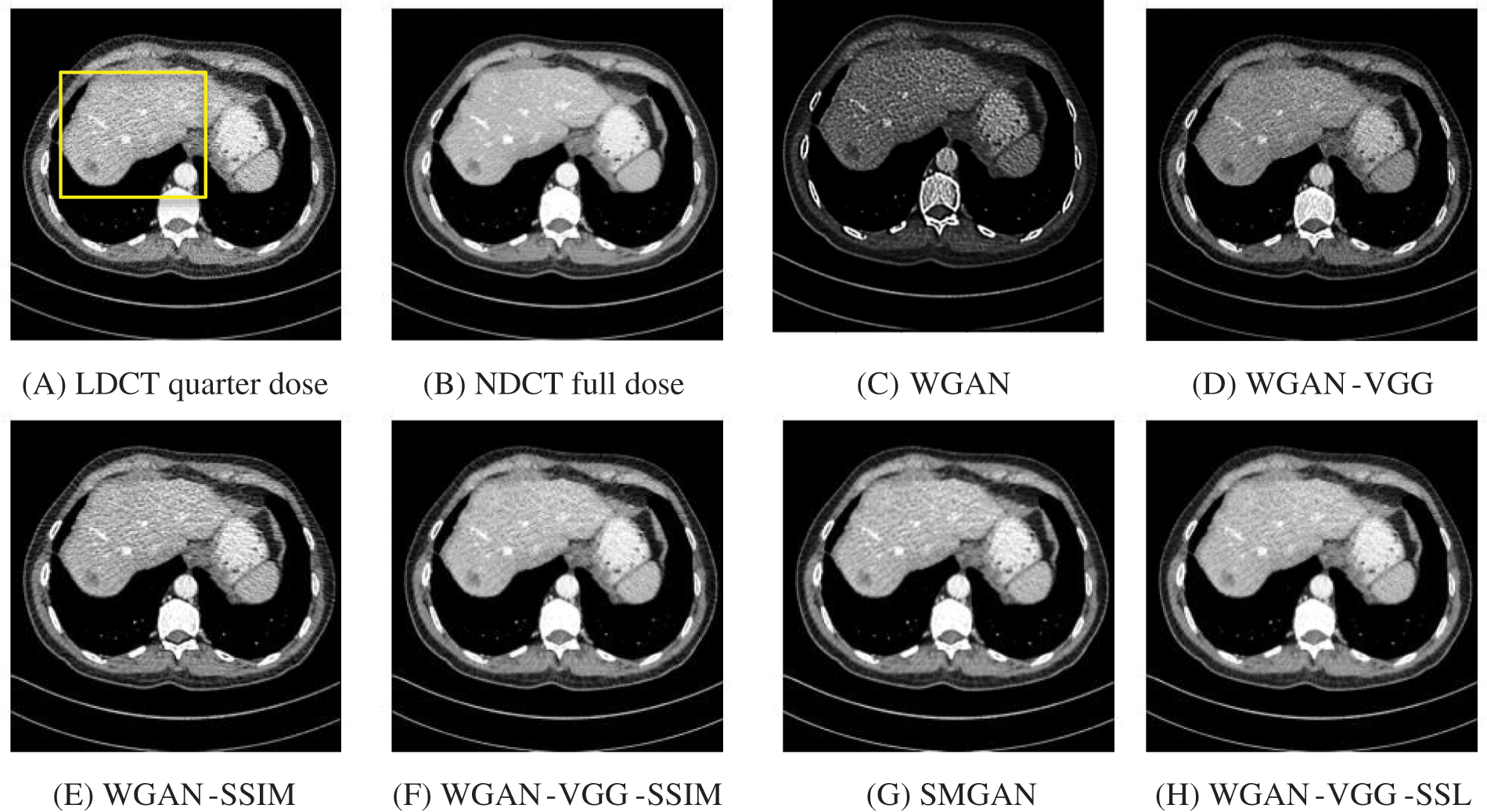
Figure 4: The generated images from the testing data ‘L067’ on GPU at 2000 iterations

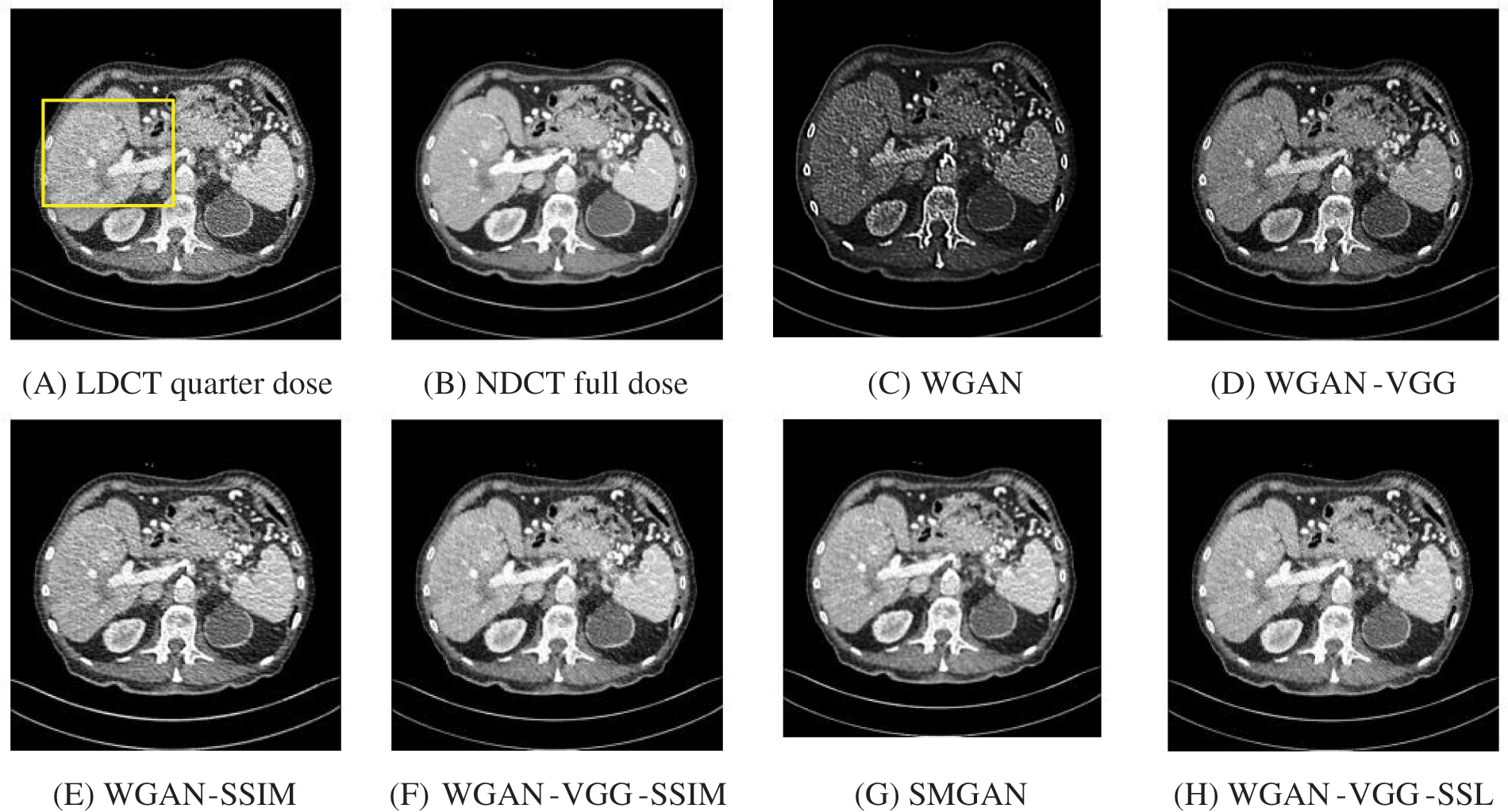
Figure 5: The generated images from the testing data ‘L506’ on GPU at 2000 iterations

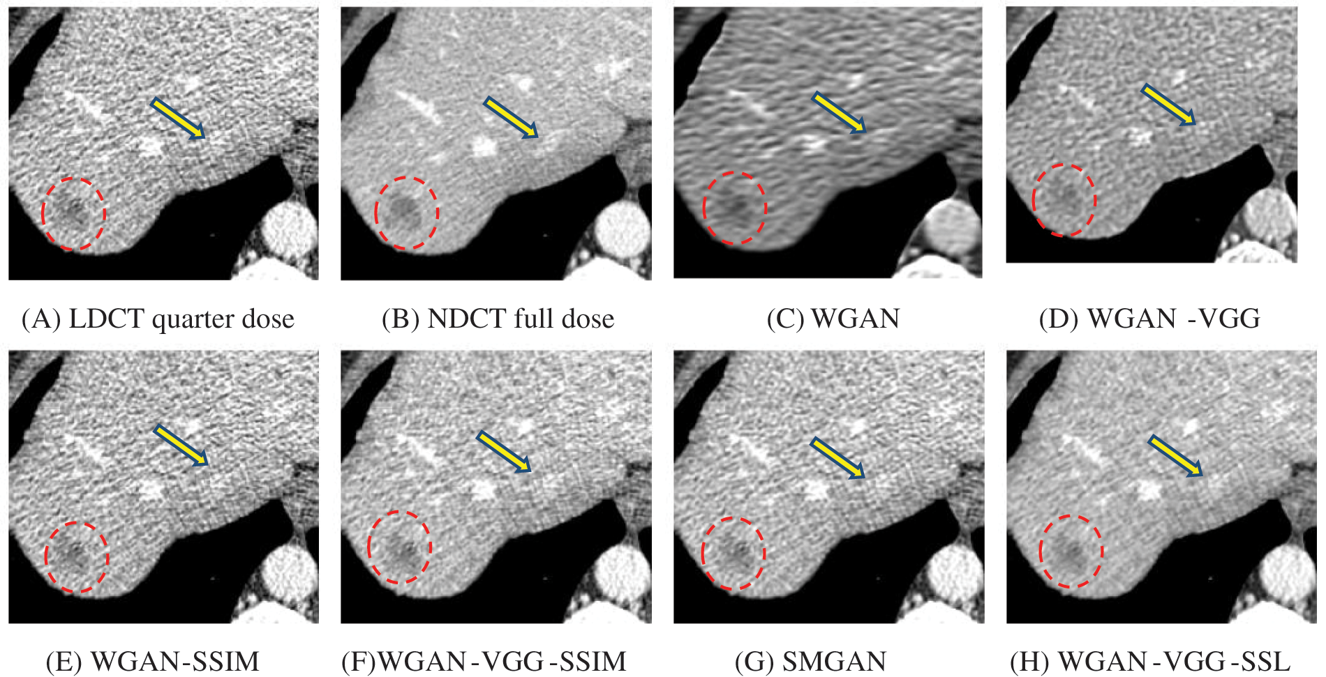
Figure 6: Zoomed slices over the yellow rectangle region of interest (ROI) in Fig. 2 represent the attenuation of liver lesions in the red circles

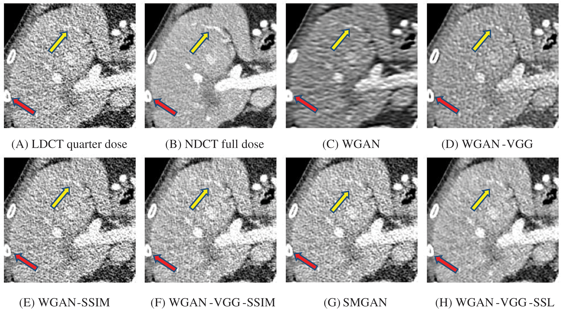
Figure 7: Zoomed slices over the yellow rectangle ROI in Fig. 3 represent a section of the abdomen CT image

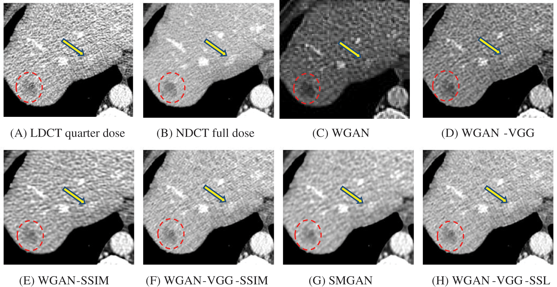
Figure 8: Zoomed slices over the yellow rectangle ROI in Fig. 4 represent the attenuation of the liver lesions in the red circles

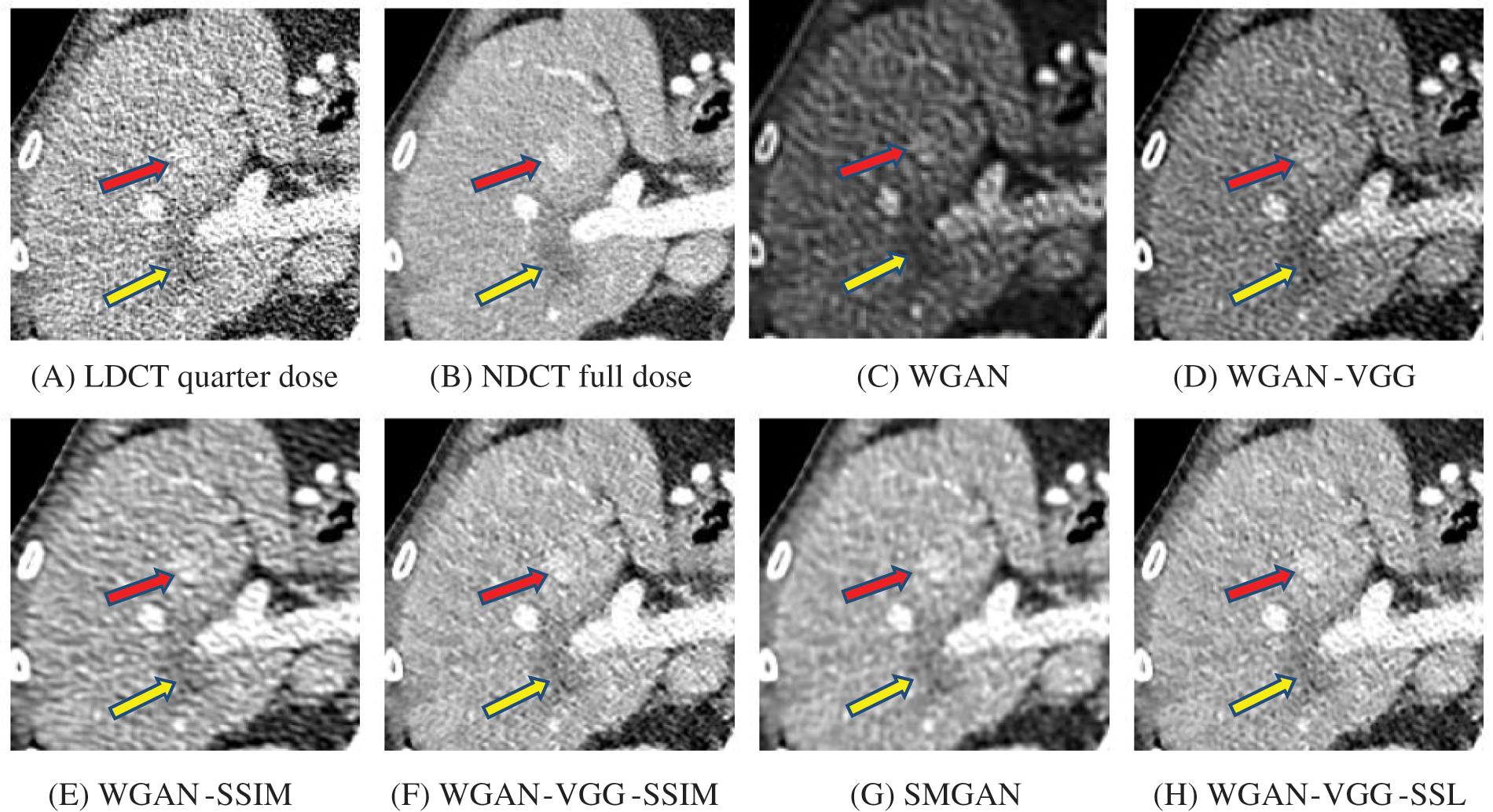
Figure 9: Zoomed slices over the yellow rectangle ROI in Fig. 5 represent a section of the abdomen CT image

4.3 Quantitative Analysis for the Performance of CPU and GPU

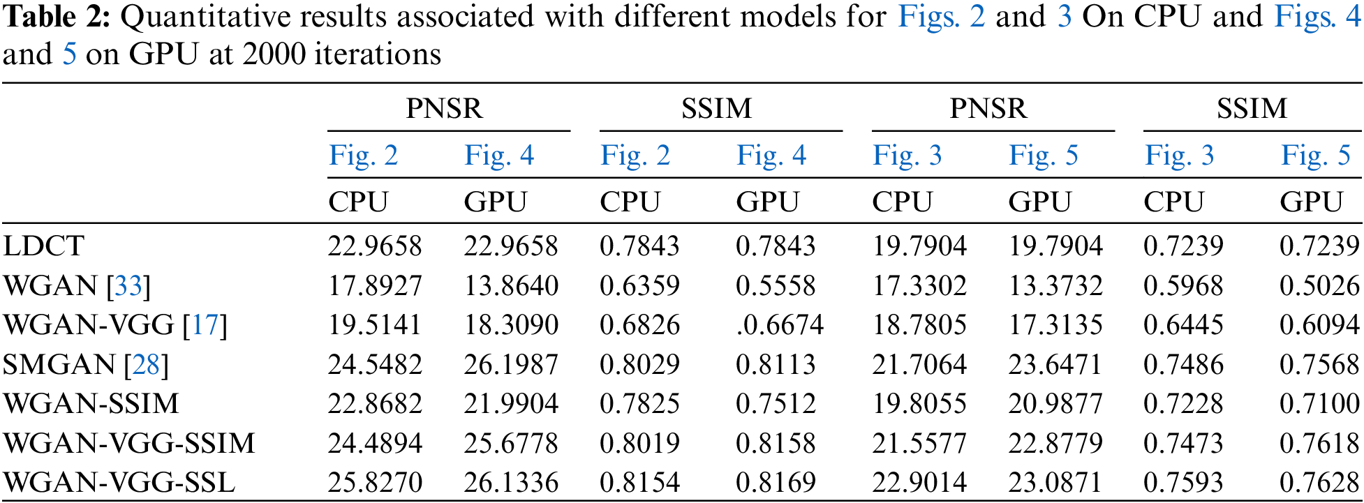
For quantitative analysis, PNSR and Structural Similarity Index Measure (SSIM) have been used to evaluate our models (WGAN-SSIM, WGAN-VGG-SSIM, and WGAN-VGG-SSL), and the best-known models WGAN, WGAN-VGG, and SMGAN, as shown in Table 2, although the training time for each model after 2000 iterations on the GPU is 20 times less than that on the CPU, the results demonstrate that the WGAN-VGG-SSL has higher SSIM values than the other models on both CPU and GPU, also has higher values of PNSR than the other models on the CPU and had close results to those obtained by the SMGAN on the GPU.

4.4 Network Convergence

This paper investigates the loss curve’s behavior for our models (WGAN-SSIM, WGAN-VGG-SSIM, and WGAN-VGG-SSL), and other known models WGAN, WGAN-VGG, and SMGAN. On CPU and GPU as shown in Fig. 10. Although WGAN and WGAN-VGG were used to improve the stability of GAN, the difference in the stability of the two models was noticed. On the CPU, the discriminator and the generator losses in WGAN are oscillating because the model is trained slowly; WGAN and WGAN-VGG are worse than the other models. In addition, on the GPU, two models WGAN and WGAN-VGG are unstable. The training oscillates in the convergence process because the models cannot find an equilibrium between the discriminator and the generator. During the training, the D loss and G loss are not consistent. They have not trained for enough time and the two models are unstable because the stability comes when the model trains both the D and the G networks simultaneously in a zero-sum game. It is noticed that our models WGAN-VGG-SSIM, WGAN-SSIM, and WGAN-VGG-SSL produced images better than those of WGAN and WGAN-VGG and converged to a stable equilibrium. WGAN-VGG-SSIM and WGAN-SSIM were less stable on the GPU than on the CPU. The three models are stable because the SSIM loss helps the G network train well. The G network generates samples like NDCT images at the end of the training. This work figured out that the D network could not classify between the model distribution and data distribution correctly. Two losses of the D and G converged fast and decreased gradually until close to zero. The WGAN-VGG-SSL model reached Nash equilibrium because the D and G networks had well adversarial training.

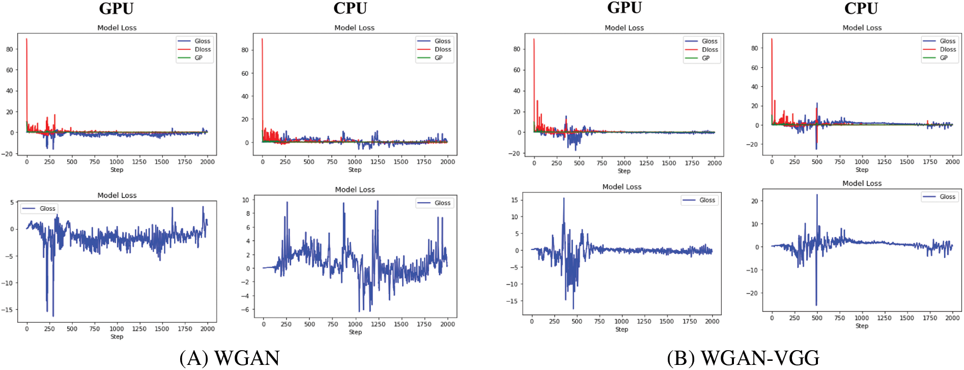
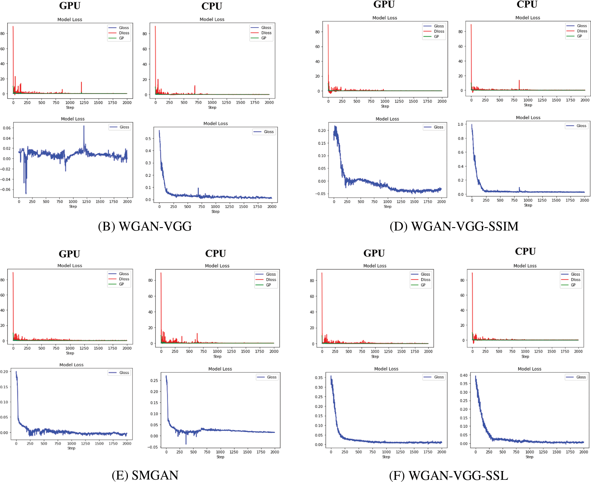
Figure 10: The stability of different models WGAN, WGAN-VGG, WGAN-SSIM, WGAN-VGG-SSIM, SMGAN, and WGAN-VGG-SSL at 2000 iterations on GPU and CPU

5  Conclusion

This study introduced three new WGAN-based models with different loss functions (WGAN-SSIM, WGAN-VGG-SSIM, and WGAN-VGG-SSL) to reduce noise and preserve important information for LDCT images and investigate the effect of different types of loss functions. Theproposed models were applied to the NIH-AAPM-Mayo Clinic LDCT images. The three models have results that quantitatively and qualitatively outperform those of the state-of-the-art models (WGAN, WGAN-VGG, and SMGAN). Experimental results demonstrated that our model WGAN-VGG-SSIM achieved better quality for LDCT image denoising compared with WGAN, WGAN-VGG, and SMGAN because of the usage of the mixed features between VGG loss and SSIM loss; WGAN-VGG-SSIM improved both the perceptual and informative structural features. The loss values of the curve during the training process of WGAN-SSIM, SMGAN, WGAN-VGG-SSIM, and WGAN-VGG-SSL are more stable and converged to a stable equilibrium than those of WGAN and WGAN-VGG. Even though WGAN-VGG-SSIM obtained better results than the state-of-the-art models, WGAN-VGG-SSL demonstrated higher quantitative and qualitative results and generated high-level image quality compared with the other denoising models because of the combination between feature domain distance and adversarial loss. It can be observed that models based on SSIM and VGG loss seem to be an ideal solution for high-quality visual images with fewer artifacts and more details. SSL loss presented an informative advantage between adjacent inter-slices. We proposed the first study comparing the performance of the WGAN denoising models on CPU and GPU. The qualitative results achieved using CPU and GPU are equivalent despite the time difference taken between them, but the proposed models are more stable on CPU than GPU. In the future, we will use more complicated network structures of the generator and different losses to obtain better results with higher quality. The CycleGAN network with determined constraints and structurally sensitive loss will be applied for the LDCT image denoising problem. Also, our denoising methods will be extended to different medical images with different noise levels to investigate how noise levels correlate with different denoising models.

Acknowledgement: The authors admit the support of the faculty of science, Assiut university.

Funding Statement: The authors received no specific funding for this study.

Conflicts of Interest: The authors declare that they have no conflicts of interest to report regarding the present study.

References

1. B. Praveen, S. Talukdar, S. Mahato, J. Mondal, P. Sharma et al., “Analyzing trend and forecasting of rainfall changes in India using non-parametrical and machine learning approaches,” Scientific Reports, vol. 10, no. 1, pp. 1–21, 2020. [Google Scholar]

2. M. A. Haq, “CDLSTM: A novel model for climate change forecasting,” CMC-Computers, Materials & Continua, vol. 71, no. 2, pp. 2363–2381, 2022. [Google Scholar]

3. M. A. Haq, “Planetscope nanosatellites image classification using machine learning,” Computer Systems Science and Engineering, vol. 42, no. 3, pp. 1031–1046, 2022. [Google Scholar]

4. M. A. Haq and M. A. R. Khan, “DNNBoT: Deep neural network-based botnet detection and classification,” CMC-Computers, Materials & Continua, vol. 71, no. 1, pp. 1729–1750, 2022. [Google Scholar]

5. S. Dargan, M. Kumar, M. R. Ayyagari and G. Kumar, “A survey of deep learning and its applications: A new paradigm to machine learning,” Archives of Computational Methods in Engineering, vol. 27, no. 4, pp. 1071–1092, 2020. [Google Scholar]

6. I. Goodfellow, J. Pouget-Abadie, M. Mirza, B. Xu, D. Warde-Farley et al., “Generative adversarial networks,” Communications of the ACM, vol. 63, no. 11, pp. 139–144, 2020. [Google Scholar]

7. I. Goodfellow, “NIPS 2016 tutorial: Generative adversarial networks,” arXiv preprint arXiv:1701.00160, pp. 1–57, 2016. [Online]. Available: https://arxiv.org/abs/1701.00160 [Google Scholar]

8. J. Zhu, Y. Shen, D. Zhao and B. Zhou, “In-domain GAN inversion for real image editing,” in Proc. of Eur. Conf. on Computer Vision, Glasgow, UK, vol. 12362, pp. 592–608, 2020. [Google Scholar]

9. P. Isola, J. -Y. Zhu, T. Zho and A. A. Efros, “Image-to-image translation with conditional adversarial networks,” in Proc. of the IEEE Conf. on Computer Vision and Pattern Recognition, Honolulu, Hawaii, USA, pp. 1125–1134, 2017. [Google Scholar]

10. C. Ledig, L. Theis, F. Huszár, J. Caballero, A. Cunningham et al., “Photo-realistic single image super-resolution using a generative adversarial network,” in Proc. of the IEEE Conf. on Computer Vision and Pattern Recognition, Honolulu, Hawaii, USA, pp. 4681–4690, 2017. [Google Scholar]

11. H. Shi, J. Dong, W. Wang, Y. Qian and X. Zhang, “SSGAN: Secure steganography based on generative adversarial networks,” in Proc. Pacific Rim Conf. on Multimedia, Harbin, China, pp. 534–544, 2017. [Google Scholar]

12. A. Radford, L. Metz and S. Chintala, “Unsupervised representation learning with deep convolutional generative adversarial networks,” arXivpreprintarXiv:1511.06434, pp. 1–16, 2015. [Online]. Available: https://arxiv.org/abs/1511.06434 [Google Scholar]

13. A. Brock, J. Donahue and K. Simonyan, “Large scale GAN training for high fidelity natural image synthesis,” arXiv Preprint arXiv, 1809.11096, pp. 1–35, 2018. [Online]. Available: https://arxiv.org/abs/1809.11096 [Google Scholar]

14. Q. Yang, P. Yan, Y. Zhang, H. Yu, Y. Shi et al., “Low-dose CT image denoising using a generative adversarial network with wasserstein distance and perceptual loss,” IEEE Transactions on Medical Imaging, vol. 37, no. 6, pp. 1348–1357, 2018. [Google Scholar] [PubMed]

15. Bhadra, W. Zhou and M. A. Anastasio, “Medical image reconstruction with image-adaptive priors learned by use of generative adversarial networks,” in Proc. Medical Imaging 2020: Physics of Medical Imaging, Houston, Texas, USA, vol. 11312, pp. 206–213, 2020. [Google Scholar]

16. K. Kamnitsas, C. Baumgartner, C. Ledig, V. Newcombe, J. Simpson et al., “Unsupervised domain adaptation in brain lesion segmentation with adversarial networks,” in Proc. Int. Conf. on Information Processing in Medical Imaging, Boone, NC, USA, pp. 597–609, 2017. [Google Scholar]

17. Y. Xue, T. Xu, H. Zhang, L. R. Long and X. Huang, “SegAN: Adversarial network with multi-scale L1 loss for medical image segmentation,” Neuroinformatics, vol. 16, no. 3, pp. 383–392, 2018. [Google Scholar] [PubMed]

18. T. Schlegl, P. Seeböck, S. M. Waldstein, U. Schmidt-Erfurth and G. Langs, “Unsupervised anomaly detection with generative adversarial networks to guide marker discovery,” in Proc. Int. Conf. on Information Processing in Medical Imaging, Boone, NC, USA, pp. 146–157, 2017. [Google Scholar]

19. T. Schlegl, P. Seeböck, S. M. Waldstein, G. Langs and U. Schmidt-Erfurth, “F-AnoGAN: Fast unsupervised anomaly detection with generative adversarial networks,” Medical Image Analysis, vol. 54, pp. 30–44, 2019. [Google Scholar] [PubMed]

20. J. G. Lee, S. Jun, Y. W. Cho, H. Lee, G. B. Kim et al., “Deep learning in medical imaging: General overview,” Korean Journal of Radiology, vol. 18, no. 4, pp. 570–584, 2017. [Google Scholar] [PubMed]

21. M. Frid-Adar, E. Klang, M. Amitai, J. Goldberger and H. Greenspan, “Synthetic data augmentation using GAN for improved liver lesion classification,” in Proc. IEEE 15th Int. Symp. on Biomedical Imaging (ISBI 2018), Washington, USA, IEEE, pp. 289–293, 2018. [Google Scholar]

22. S. Liu, Y. Wang, X. Yang, B. Lei, L. Liu et al., “Deep learning in medical ultrasound analysis: A review,” Engineering, vol. 5, no. 2, pp. 261–275, 2019. [Google Scholar]

23. H. Chen, Y. Zhang, M. K. Kalra, F. Lin, Y. Chen et al., “Low-dose CT with a residual encoder-decoder convolutional neural network,” IEEE Transactions on Medical Imaging, vol. 36, no. 12, pp. 2524–2535, 2017. [Google Scholar] [PubMed]

24. K. Simonyan and A. Zisserman, “Very deep convolutional networks for large-scale image recognition,” arXiv preprint arXiv:1409.1556, pp. 1–14, 2014. [Online]. Available: https://arxiv.org/abs/1409.1556 [Google Scholar]

25. C. You, Q. Yang, H. Shan, L. Gjesteby, G. Li et al., “Structurally-sensitive multi-scale deep neural network for low-dose CT denoising,” IEEE Access, vol. 6, pp. 41839–41855, 2018. [Google Scholar] [PubMed]

26. G. Wang and X. Hu, “Low-dose CT denoising using a progressive wasserstein generative adversarial network,” Computers in Biology and Medicine, vol. 135, pp. 104625–104640, 2021. [Google Scholar] [PubMed]

27. H. Zhao, O. Gallo, I. Frosio and J. Kautz, “Loss functions for image restoration with neural networks,” IEEE Transactions on Computational Imaging, vol. 3, no. 1, pp. 47–57, 2016. [Google Scholar]

28. M. Arjovsky and L. Bottou, “Towards principled methods for training generative adversarial networks,” arXiv preprint arXiv:1701.04862, pp. 1–17, 2017. [Online]. Available: https://arxiv.org/abs/1701.04862 [Google Scholar]

29. T. Salimans, I. Goodfellow, W. Zaremba, V. Cheung, A. Radford et al., “Improved techniques for training GANs,” Advances in Neural Information Processing Systems, Barcelona, Spain, vol. 29, pp. 1–9, 2016. [Google Scholar]

30. I. Gulrajani, F. Ahmed, M. Arjovsky, V. Dumouli and A. Courville, “Improved training of wasserstein GANs,” Advances in Neural Information Processing Systems, Long Beach, CA, USA, vol. 30, pp. 5768–5778, 2017. [Google Scholar]

31. A. Manduca, L. Yu, J. D. Trzasko, N. Khaylova, J. M. Kofler et al., “Projection space denoising with bilateral filtering and CT noise modeling for dose reduction in CT,” Medical Physics, vol. 36, no. 11, pp. 4911–4919, 2009. [Google Scholar] [PubMed]

32. A. K. Hara, R. G. Paden, A. C. Silva, J. L. Kujak, H. J. Lawder et al., “Iterative reconstruction technique for reducing body radiation dose at CT: Feasibility study,” American Journal of Roentgenology, vol. 193, no. 3, pp. 764–771, 2009. [Google Scholar] [PubMed]

33. J. Ma, J. Huang, Q. Feng, H. Zhang, H. Lu et al., “Low-dose computed tomography image restoration using previous normal-dose scan,” Medical Physics, vol. 38, no. 10, pp. 5713–5731, 2011. [Google Scholar] [PubMed]

34. J. M. Wolterink, T. Leiner, M. A. Viergever and I. Išgum, “Generative adversarial networks for noise reduction in low-dose CT,” IEEE Transactions on Medical Imaging, vol. 36, no. 12, pp. 2536–2545, 2017. [Google Scholar] [PubMed]

35. H. Chen, Y. Zhang, W. Zhang, P. Liao, K. Li et al., “Low-dose CT via convolutional neural network,” Biomedical Optics Express, vol. 8, no. 2, pp. 679–694, 2017. [Google Scholar] [PubMed]

36. E. Kang, J. Min and J. C. Ye, “A deep convolutional neural network using directional wavelets for low-dose X-ray CT reconstruction,” Medical Physics, vol. 44, no. 10, pp. e360–e375, 2017. [Google Scholar] [PubMed]

37. L. Ma, H. Xue, G. Yang, Z. Zhang, C. Li et al., “SCRDN: Residual dense network with self-calibrated convolutions for low dose CT image denoising,” Nuclear Instruments and Methods in Physics Research Section A: Accelerators, Spectrometers, Detectors and Associated Equipment, vol. 1045, pp. 167625–167632, 2023. [Google Scholar]

38. X. Yi and P. Babyn, “Sharpness-aware low-dose CT denoising using conditional generative adversarial network,” Journal of Digital Imaging, vol. 31, no. 5, pp. 655–669, 2018. [Google Scholar] [PubMed]

39. Y. Ma, B. Wei, P. Feng, P. He, X. Guo et al., “Low-dose CT image denoising using a generative adversarial network with a hybrid loss function for noise learning,” IEEE Access, vol. 8, pp. 67519–67529, 2020. [Google Scholar]

40. S. Y. Jeon, W. Kim and J. H. Choi, “MM-Net: Multi-frame and multi-mask-based unsupervised deep denoising for low-dose computed tomography,” IEEE Transactions on Radiation and Plasma Medical Sciences, pp. 1–12, 2022. [Google Scholar]

41. Z. Yin, K. Xia, S. Wang, Z. He, J. Zhang et al., “Unpaired low-dose CT denoising via an improved cycle-consistent adversarial network with attention ensemble,” The Visual Computer, pp. 1–22, 2022. [Google Scholar]

42. Q. Yang, P. Yan, M. K. Kalra and G. Wang, “CT image denoising with perceptive deep neural networks,” arXiv preprint arXiv:1702.07019, pp. 1–8, 2017. [Online]. Available: https://arxiv.org/abs/1702.07019 [Google Scholar]

43. V. Nair and G. E. Hinton, “Rectified linear units improve restricted boltzmann machines,” in Proc. of the 27 Int. Conf. on Machine Learning, Haifa, Israel, pp. 807–814, 2010. [Google Scholar]

44. AAPM, “Low dose CT grand challenge,” 2017. [Online]. Available: http://www.aapm.org/GrandChallenge/LowDoseCT/# [Google Scholar]

45. D. P. Kingma and J. Ba, “Adam: A method for stochastic optimization,” arXiv preprint arXiv:1412.6980, pp. 1–15, 2014. [Online]. Available: https://arxiv.org/abs/1412.6980 [Google Scholar]