
 Submit a Paper
 Propose a Special lssue
 Open Access
ARTICLE

Fault Diagnosis of Power Transformer Based on Improved ACGAN Under Imbalanced Data
1 School of Electrical Engineering, Xinjiang University, Urumqi, 830047, China
2 School of Mathematics, Xinjiang University, Urumqi, 830047, China
* Corresponding Author: Xiaojing Ma. Email:
Computers, Materials & Continua 2023, 75(2), 4573-4592. https://doi.org/10.32604/cmc.2023.037954
Received 12 November 2022; Accepted 13 February 2023; Issue published 31 March 2023
 View Full Text
 Download PDF
Abstract
The imbalance of dissolved gas analysis (DGA) data will lead to over-fitting, weak generalization and poor recognition performance for fault diagnosis models based on deep learning. To handle this problem, a novel transformer fault diagnosis method based on improved auxiliary classifier generative adversarial network (ACGAN) under imbalanced data is proposed in this paper, which meets both the requirements of balancing DGA data and supplying accurate diagnosis results. The generator combines one-dimensional convolutional neural networks (1D-CNN) and long short-term memories (LSTM), which can deeply extract the features from DGA samples and be greatly beneficial to ACGAN’s data balancing and fault diagnosis. The discriminator adopts multilayer perceptron networks (MLP), which prevents the discriminator from losing important features of DGA data when the network is too complex and the number of layers is too large. The experimental results suggest that the presented approach can effectively improve the adverse effects of DGA data imbalance on the deep learning models, enhance fault diagnosis performance and supply desirable diagnosis accuracy up to 99.46%. Furthermore, the comparison results indicate the fault diagnosis performance of the proposed approach is superior to that of other conventional methods. Therefore, the method presented in this study has excellent and reliable fault diagnosis performance for various unbalanced datasets. In addition, the proposed approach can also solve the problems of insufficient and imbalanced fault data in other practical application fields.Keywords
Oil-immersed power transformers, as one of the power grid’s core pieces of equipment, play a critical role in power transmission and distribution. The operation of an oil-immersed power transformer is often affected by the harsh operating environment, and once the fault occurs, there will be many accidents of various sizes, ranging from small-scale power outages to fires and explosions, resulting in immeasurable economic losses and casualties [1,2]. Therefore, whether the oil-immersed transformer can be judged accurately in time has an important practical significance [3].
When there are electrical and thermal faults in the oil-immersed transformer, a chemical reaction will occur in the fault area leading to cracking, which will produce characteristic gases related to the type of transformer fault and gradually dissolve in the transformer oil, mainly including hydrogen (H2), methane (CH4), acetylene (C2H2), ethylene (C2H4), and ethane (C2H6), which are the five characteristic gases [4,5]. If the dissolution rate of oil is less than the production rate of characteristic gas, excess characteristic gas will diffuse inside the transformer. DGA technology is used to judge whether there are faults and fault types in transformers by monitoring the composition and concentration of characteristic gases generated during the operation of oil-immersed transformers, which has become the preferred method for monitoring on line in China and abroad [6].
For the past decades, Various diagnostic methods have been developed based on DGA techniques, including the international electrotechnical commission (IEC), the improved three ratios method (ITR), the Duval triangle method (DTM), etc. The above traditional DGA methods mainly use empirical assumptions and the practical experience of experts to establish a diagnosis rule based on the “code-type of fault” relationship between the concentration or ratio of the characteristic gas and the type of transformer fault. The lack of diagnostic accuracy. With the rapid development of artificial intelligence (AI) and machine learning (ML), intelligent models based on the combination of DGA technology and shallow machine learning are directly or indirectly used in transformer fault diagnosis, such as the artificial neural network (ANN), the fuzzy system (FS), the support vector machine (SVM), etc. Yang et al. combines the bat algorithm (BA) and probabilistic neural networks (PNN) to propose a transformer fault diagnosis model based on BA-PNN, which has significant advantages in pattern classification [7]. Malik et al. proposed a fuzzy reinforcement learning (RL) based intelligent classifier for power transformer incipient faults that can progressively learn to identify faults with high accuracy for all fault types, thus solving the problem of low recognition accuracy of existing fault classifiers [8]. Hong et al. proposed a new SVM-based framework for transformer fault diagnosis that applied a multi-step feature extraction process composed of characteristic gas concentrations and their ratios. Based on the characteristic distribution of each sample, a suitable support vector machine multi-classification method was proposed using a hierarchical decision tree structure. It solves the problem that the traditional SVM multi-classification method and parameter optimization algorithm have low training efficiency [9]. Although the above methods have improved the accuracy of transformer fault diagnosis to a certain extent, it has been confirmed that the learning abilities of shallow machine learning methods are ultimately limited as convention machine learning methods are difficult to dig out the deeper microfeatures in DGA data due to weak feature extraction ability. In 2006, Professor Hinton et al. proposed the concept of deep learning (DL), which has since set off the third wave of artificial intelligence [10]. Nowadays, deep learning algorithms like CNN and LSTM, which are the most popular data-driven model algorithms, have a high demand for the number of training samples. When most deep learning models deal with fault classification problems, they will make the training samples of each fault type reach equilibrium to avoid the problem that a certain fault type is ignored by the neural network due to a lack of samples [11]. However, the oil-immersed transformer has a low fault incidence and rare fault type samples, which limits the operation efficiency and research directions for transformer fault diagnosis at present. Generalization ability of the diagnosis model is limited and it cannot guarantee accurate transformer fault assessment [12]. Therefore, one of the key issue is how to use the generative model to solve the adverse effects of imbalanced data.
At present, the methods to deal with unbalanced data can be divided into two categories: one is to achieve the data set balance by changing the data distribution before training the classifier, among which the sampling method is the most commonly used; the other is to improve the learning algorithm to make it suitable for unbalanced data classification, and the most common method is Boosting. Sampling methods mainly include the common sampling method and the synthetic sampling method. The normal sampling methods include undersampling and oversampling. Undersampling balances the data by discarding some of the majority of the oversampling samples, but does so at the loss of potentially useful information. Oversampling reduces the disequilibrium of the dataset by simply replicating a few class samples, but increases the overfitting risk of the model. Therefore, the synthetic minority oversampling technique (SMOTE) is put forward. This method avoids the overfitting problem in random oversampling, but SMOTE does not take into account the overall distribution of the data. So the sample generation mechanism has a certain blindness. The most common improvement method based on Boosting is the AdaBoost algorithm, which can be directly used for classifying unbalanced data sets. In each iteration process, AdaBoost will increase the weight of the samples that are not correctly classified and decrease the weight of the samples that are correctly classified. This makes the classifier trained by the system in the next iteration pay more attention to the wrong samples classified by the existing classifiers and improve the classification effect of these samples. Because small class samples are more likely to be misclassified, the AdaBoost algorithm can improve the classification performance for small class samples. However, the AdaBoost algorithm does not take the influence of unbalanced samples from different categories into account and adopts identical weighting strategy for wrong classified samples. When the data set contains samples that are hard to be classified correctly from majority classes, the assigned weights for those samples will become larger as the increasing of training iterations. As a result, the obtained classifier will become more sensitive to those samples and result in poor classification performance for samples from minority classes.
In October 2014, Goodfellow et al. of the University of Montreal proposed an emerging implicit density generation model, the generative adversarial network (GAN), which is based on the traditional generation network [13]. Since its introduction, GAN has been widely used in computer vision [14], text generation [15], and target detection [16]. However, at the same time, GAN will be difficult to control training and prone to mode collapse. In response to these problems, researchers have proposed hundreds of GAN variant models in just a few years, such as Wasserstein GAN (WGAN) [17], conditional GAN (CGAN) [18], and deep convolution GAN (DCGAN) [19], and applied them to fault diagnosis. Li introduced the strategy gradient algorithm in GAN to realize the expansion of the transformer oil chromatographic case and put the expanded data into the back propagation neural network (BPNN) for fault classification [20]. Liu et al. introduced the Wasserstein distance and gradient penalty algorithm into CGAN to guide the generation process of multi-class transformer fault samples and established a stack self-encoder diagnostic model for fault diagnosis [21]. Fang et al. proposed to build a GAN to generate synthetic samples for a small subset of labeled samples, which solved the problem that traditional supervised learning methods could not learn information from unlabeled sample data and improved the accuracy of transformer fault classification [22]. Although the above method can generate part of the data through GAN to solve the imbalance of data and then use the classification model for fault diagnosis, this will lead to more complexity of the fault diagnosis process. In addition, the model training time will get longer and a suitable classifier is needed to tackle the value of the balanced data.
Since the constraint of generators on discriminators in GAN and variant models leads to a reduction in the final diagnostic accuracy, most GAN researchers abandon the use of discriminators as the final fault classifier. In view of the above problems, a novel transformer fault diagnosis method based on improved ACGAN under imbalanced data is proposed in this paper, which meets both the requirements of balancing DGA data and supplying accurate diagnosis results. The generator combines 1D-CNN and LSTM, while the discriminator adopts MLP. The experimental results indicate that the presented method can effectively mitigate the adverse effects of data imbalance on the deep learning model and improve the accuracy of the transformer fault diagnosis test. Moreover, it can also fully tap the potential of the discriminator as the main classifier in ACGAN and provide a new approach for handling imbalance and insufficient of data in practical application.
The rest of this paper is organized as follows: Section 2 introduces the relevant technical background and proposes a fault diagnosis model. Section 3 introduces the DGA data processing process. Section 4 presents six sets of comparative experiments, with analysis and discussion of the results. Finally, we conclude this paper in Section 5.
2 Basic Theory of Fault Diagnosis Model
The basic structure of the GAN model is shown in Fig. 1, which consists of a generator network (G) and a discriminator network (D). Both of them adopt fully-connected layer neural networks and are independent of each other, which has the advantages of a small calculation and dataset training process. The input of G is a random noise z, which applies Gaussian noise vector generally. There are two inputs for discriminator D, one of which is real sample Xreal, and the other is pseudo sample Xfake generated by G. In GAN, the tasks for G and D are described as follow: the task of G is to generate Xfake of the similarity approximation Xreal by learning the distribution of Xreal to deceive D. While the task of D is to identify as much as possible whether the input sample is Xreal or Xfake generated by G and then output a probability value by D as the identification result [23]. When the input of D is equal to Xreal, the output of D will be equal to 1. Otherwise, the output of D is set to 0. D feedbacks the output results to G and D to update the network parameters in turn to enhance the ability of G and D.
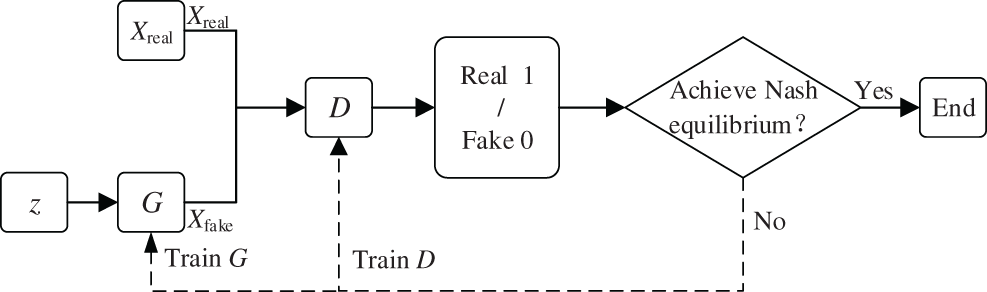
Figure 1: Basic structure of GAN model
The objective function of GAN is calculated as Eq. (1):
where, θ and ω are the parameters of G and D, respectively. E represents expectation, Pdata (x) represents the real sample distribution, and Pz (x) represents the generated sample distribution.
Throughout the process, G and D are trained against each other for the purpose of iterative optimization, so that the maximum possible approximation of G to makes D work harder to identify the truth of the sample, and the entire optimization process of the model is defined as a binary minimal-extreme game problem. In addition, G and D achieve the purpose of iterative optimization by adversarial training, so that the maximum likelihood of G is close to Pdata (x) which means Pz (x) equals to Pdata (x), and D makes more efforts to identify the true and false samples. The whole optimization process of the model is defined as a two-player minimax game. The GAN model reaches Nash equilibrium when the probability of each output of D is essentially one-half [24].
In order to solve the problem that the original GAN generation process is too free to control the training process, ACGAN is proposed in [25]. The basic structure of the model is shown in Fig. 2. Compared with the original GAN, the ACGAN not only has a random noise z at the input end of G but also adds a class label (c) as a conditional probability to change G, and D takes Xreal and Xfake as inputs. This improvement enables GAN networks to generate the required label data. There are two outputs in the D of ACGAN, one of which determines whether the input sample is from Xreal or Xfake by the Sigmod activation function; the other output is fault classification by the Softmax multi-classifier. Therefore, AGGAN not only can generate the required label data but also can be applied to the actual fault classification problem.
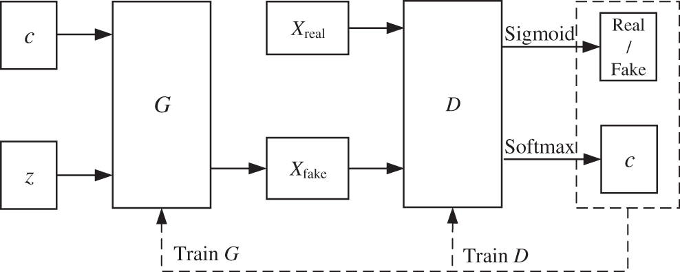
Figure 2: Basic structure of ACGAN model
The objective functions for ACGAN training are calculated as in Eqs. (2) and (3).
where, the loss function of ACGAN is composed of the loss function Ls, which characterizes whether the data is true or false. The loss function Lc is used to characterize the accuracy of data classification. The objective function of the generator is to maximize the value of (LC − LS), while the objective function of the discriminator is to maximize the value of (LC + LS), which are shown as in Eqs. (4) and (5), respectively.
2.3 Basic Theory of Improved ACGAN
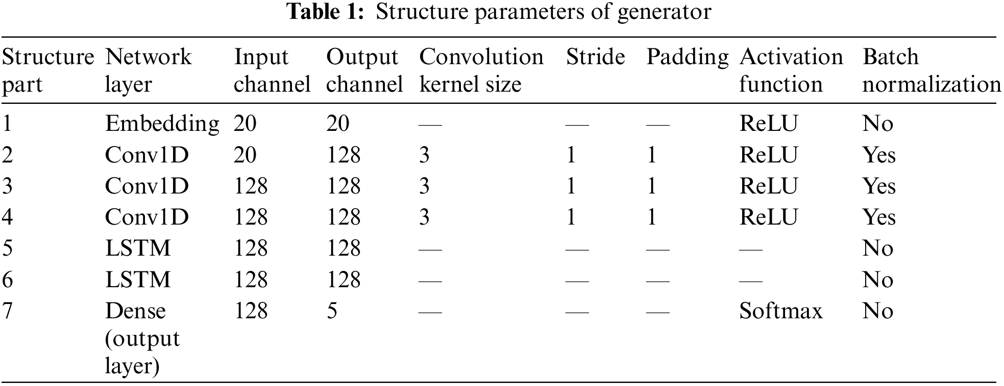
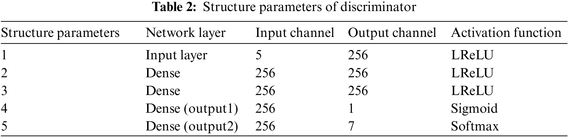
In general, the transformer fault diagnosis model based on improved ACGAN can be divided into two major parts: a generator network composed of 1D-CNN-LSTM and a discriminator network consisted by MLP. The structures of generator and discriminator are shown as Figs. 3 and 4, respectively.
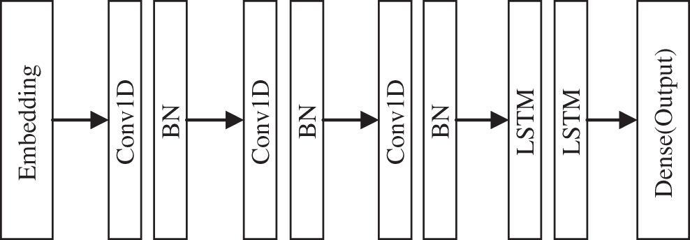
Figure 3: Basic structure of generator
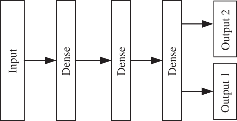
Figure 4: Basic structure of discriminator
In terms of the generator, 1D-CNN and LSTM are combined, and the whole generator model adopts an end-to-end learning architecture to improve the fault classification accuracy of the whole model. The combination of different neural networks turns it into a deep network, which enhances the nonlinearity of the model and avoids the over-fitting phenomenon during model training. Moreover, the combined model is able to effectively learn the mathematical distribution and feature information of DGA data, so that the generated data are closer to the real data. In terms of the discriminator, the MLP composed of fully connected layer neural networks can speed up the training of the model and prevent the shortcoming of losing vital features of the DGA data when the discriminator performs discrimination due to the overly complex and deep layers of the network.
The general CNN (e.g., LeNet-5) processes data in a two-dimensional format of m × n. However, the dataset used in this paper is the value of five characteristic gases of DGA samples, i.e., the format of m × 1, which is one-dimensional in space. Therefore, CNN should choose the 1D-CNN model with a more compact structure and more suitable for limited data, in which the convolution kernels use the corresponding one-dimensional convolution kernels to extract multiple features, which can significantly reduce the computation. The convolutional kernel plays a decisive role in the convolutional layer of CNN, and it is experimentally proven that the size of the convolutional kernel is best set to 3. Since the numbers and dimensions of DGA samples are small and uncomplicated, the 1D-CNN model designed in this paper uses three convolution layers and cancels the pooling layer. The pooling layer will reduce the dimension of the data to a low dimension and miss much feature information, which leads to a decrease in model accuracy. A batch normalization (BN) layer is added behind each convolution layer to improve the gradient flowing through the network, prevent the gradient from disappearing, enhance the diversity of the generated samples, and improve the stability of the training network. The generator structure parameters are shown in Table 1.
The discriminator structure parameters are shown in Table 2. The three-layer fully connected layer neural network of the discriminator selects the LeakyReLU activation function, and the gradient alpha of the left half of the function is set to 0.2. There are two outputs in the output layer. One output uses the Sigmod activation function to map the input DGA data between 0 and 1, which is used to judge the reliability of the input data. If the output is 1, which indicates the data is true and vice versa. The other output is the discrimination result of the seven fault types of the transformer as determined by the Softmax classifier.
The fault diagnosis network framework of the method in this paper is shown in Fig. 5.
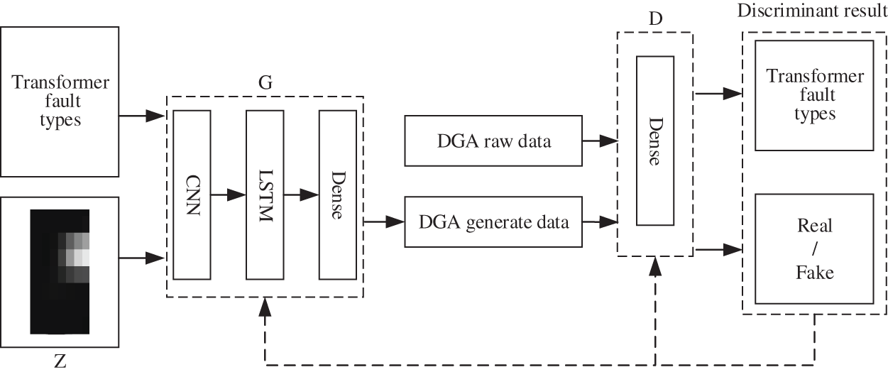
Figure 5: Framework of fault diagnosis method based on improved ACGAN
3 Data Preparation and Preprocessing
In this study, the fault diagnosis model is built based on the Anaconda distribution platform and Python 3.6.6 is adopted to establish all fault diagnosis models. While PyTorch is employed as the deep learning framework. In addition, a DELL workstation with Core i7-9700 K and NVIDIA GeForce RTX 3060 is used to implement computation and experiments.
The DGA dataset in this paper comes from domestic and foreign public datasets and related literature. In view of missing characteristic data of DGA samples, no labels, wrong classified and so on, it is necessary to preprocess the raw DGA samples before calculation. 1758 sets of DGA data, including 400 normal samples and 1358 faulty samples, are selected to establish fault diagnosis model after preprocessing. The sample distribution of each working condition is shown in Table 3.
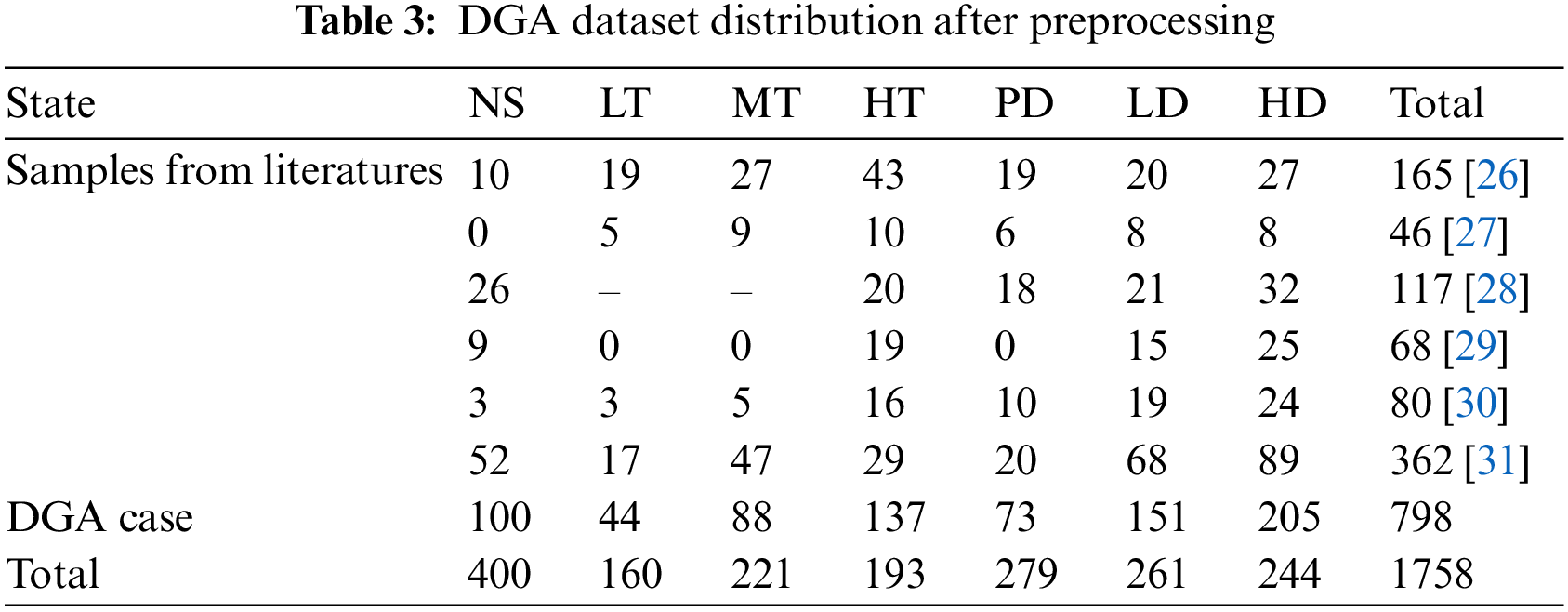
Two main working operations, including normal state (NS) and fault state (FS) are taken into account in this study. The fault condition is classified as “discharge” or “overheating.” The discharge fault is divided into low-energy discharge (LD), high-energy discharge (HD), and partial discharge (PD) according to the energy density. According to the order of temperature from low to high, overheating faults can be divided into low-temperature overheat (LT) (below 300°C), middle-temperature overheat (MT) (300–700°C), and high-temperature overheat (HT) (above 700°C). There are seven types of failures in total. The selected DGA dataset is divided into training set (80% of whole samples) and testing set (20% of whole samples). The former is used for data generation and classifier training, and the latter is used to test the classifier performance.
Normalization is a critical step for fault diagnosis due to large dispersion of raw DGA values. A fault diagnosis model without normalization will decelerate converge speed and reduce classification accuracy. Moreover, to prevent the “big numbers swallowing decimals” of raw DGA data, the original data is normalized to the (0, 1) interval by the dispersion standardization method to eliminate the influence on fault diagnosis results, as shown in Eq. (6).
where,
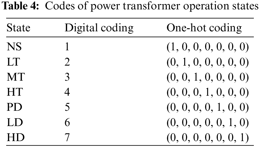
Generally, in order to facilitate the diagnosis model’s ability to effectively extract features and calculate loss function in the training process, one-hot coding is used to label all kinds of operation states of transformers in turn, as shown in Table 4. In this paper, the embedding layer is used in the generator part to splice and fuse the input random noise and fault category labels. The embedding layer can be seen as a similar form to one-hot coding, but its advantage over one-hot coding is that the variable generated by the embedding layer is not a specified position of 1, the other form being 0, but the value of each position is a floating-point number. In short, the embedding layer is a fully connected layer with one-hot coding as the input and the middle layer node as the vector dimension, and it can perform dimension enhancement and dimension reduction as required.
4 Fault Diagnosis Based on Improved ACGAN Under Imbalance Data
4.1 Basic Process for Fault Diagnosis
This paper has four parts based on the basic process of improving the ACGAN transformer fault diagnosis model: the training of the discriminator network, the training of the generator network, DGA sample generation, and transformer fault diagnosis. The fault diagnosis process based on improved ACGAN is shown in Fig. 6.
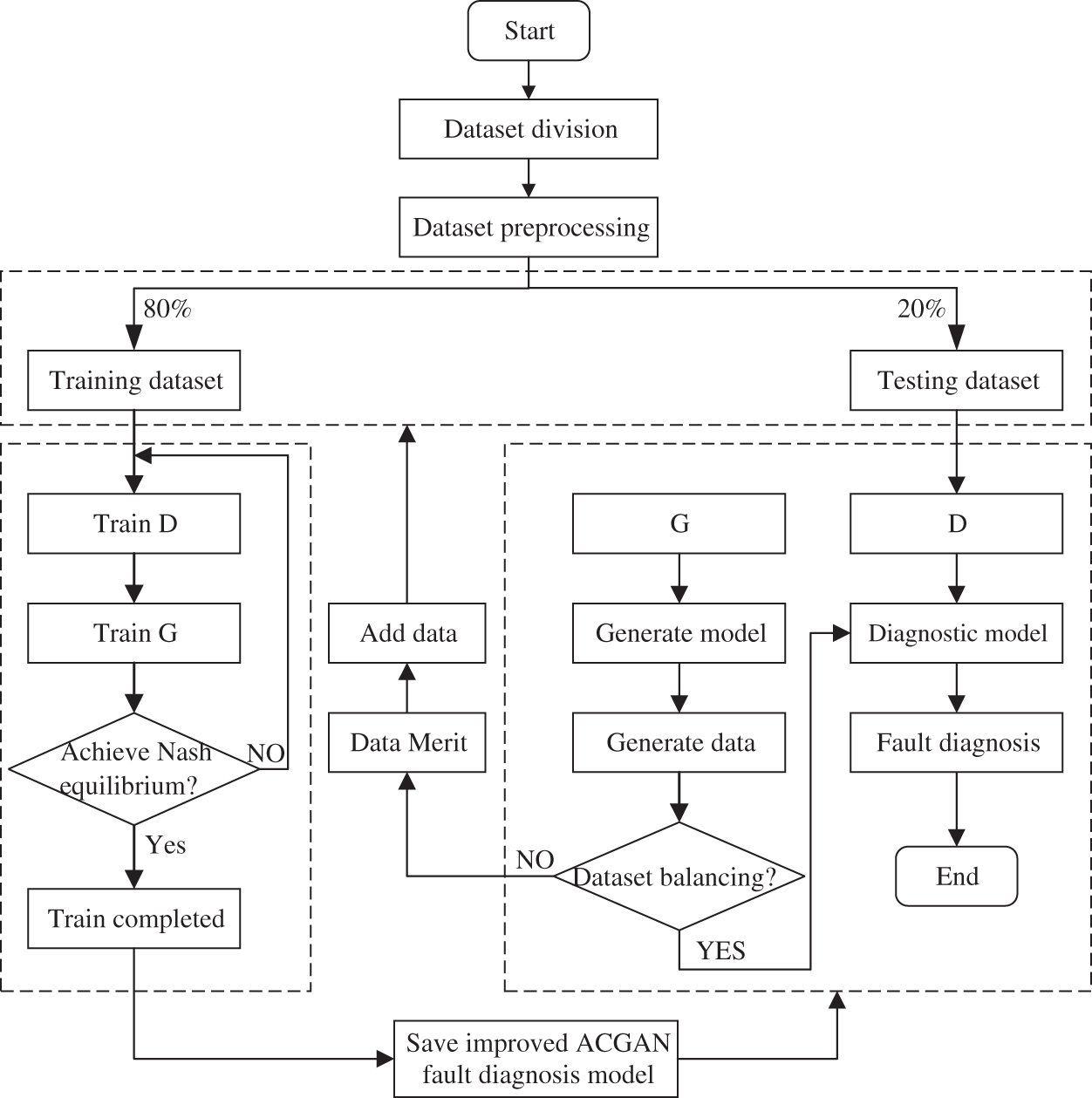
Figure 6: Framework of fault diagnosis method based on improved ACGAN
The precise processes can be described as follows:
• Step 1: Select the random noise Z and the transformer fault type label as the inputs to G to obtain the generated dataset. Then, 80% of samples are selected randomly from the DGA dataset as the model’s training dataset.
• Step 2: Use the real dataset Xreal and the generated fake dataset Xfake as inputs for D. Afterwards, calculate the loss of D and update the parameters of D.
• Step 3: Reselect random noise z and transformer fault type label c as the inputs of G to generate the fake dataset Xfake, and take the real dataset Xreal and the generated dataset Xfake as inputs of D; and calculate the loss of G and update the parameters of G.
• Step 4: Determination of the Nash equilibrium. If the Nash equilibrium is not reached, return to Step 1 and finally reach the Nash equilibrium by continuously optimizing the model parameters of D through the binary minimax game mechanism; if the Nash equilibrium is reached, G and D are trained, and the trained model parameters are saved.
• Step 5: The remaining 20 percent of the DGA dataset after the selection is used as the testing dataset for the model. The testing dataset is input into the trained fault diagnosis model, and the fault discriminant results are output by D. If the DGA dataset is unbalanced, the dataset generated by G can be added to the diagnostic dataset to expand the fault dataset, and then build more effective fault diagnosis model.
4.2 Parameters Setting for Fault Diagnosis Model
Hyperparameters are generally used to determine some parameters of the model by the empirical method for specific problems. To promote diagnosis performance of the deep learning algorithm model, the super-parameters need to be continuously adjusted to find the network parameters that allow the model to predict the most accurately. Such factors as the number of layers in the neural network, the optimization method, the learning rate, the batch size of the dataset, and the number of training rounds will affect the classification accuracy and total time of the fault diagnosis model. After repeated checking and testing, the model parameters are adjusted, and the final hyperparameters of the improved ACGAN model are shown in Table 5.
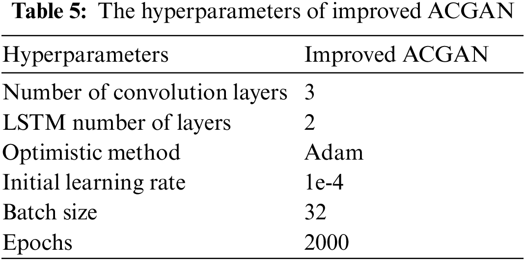
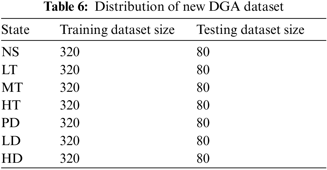
Adam optimizer, which can dynamically adjust the learning rate of each parameter of the model within a limited range, is selected to build optimization function. The batch size controls the accuracy and convergence of the model. The learning rate controls the speed of updating the model parameters. The correct choice of epochs can make the gradient’s descent direction more accurate. To mitigate the negative effects of imbalanced data on the model, the DGA dataset generated by the improved ACGAN model is filtered, and some of the generated datasets are randomly selected and added to the original DGA dataset so that the data of each fault type is consistent with the number of normal types. The distribution of the new DGA dataset is shown in Table 6.
5 Fault Diagnosis Experiments and Results Analysis
In this paper, six groups of comparative experiments are used to demonstrate the superiority of the proposed method. The main contents of experiments mentioned above are described briefly as follow:
At first, a comparative experiment based on the improved ACGAN model before and after dataset balance is conducted (experiment 1). Then, we compare the diagnosis performance between the improved ACGAN model and the ACGAN model (experiment 2), the improved ACGAN model and the traditional gas concentration ratio (experiment 3), the improved ACGAN model and the traditional machine learning model (experiment 4), and the improved ACGAN model and the traditional deep learning model (experiment 5). Finally, we evaluate the fault diagnosis performance of the proposed method based on two different actual datasets (experiment 6).
5.1 Results and Analysis of Experiment 1
Comparison of fault diagnosis performance based on AdaBoost-SVM, AdaBoost-K-Nearest Neighbor(KNN), improved ACGAN models with data imbalanced and the improved ACGAN models with data balanced, were employed to implement experiments to verify the effectiveness of the proposed approach in this paper. In this experiment, the models mentioned above were implemented five times before and after data balancing, respectively. The fault diagnosis accuracy of the five experiments mentioned above was recorded and the average accuracy was applied as the final diagnosis performance. The experimental results are shown in Table 7.
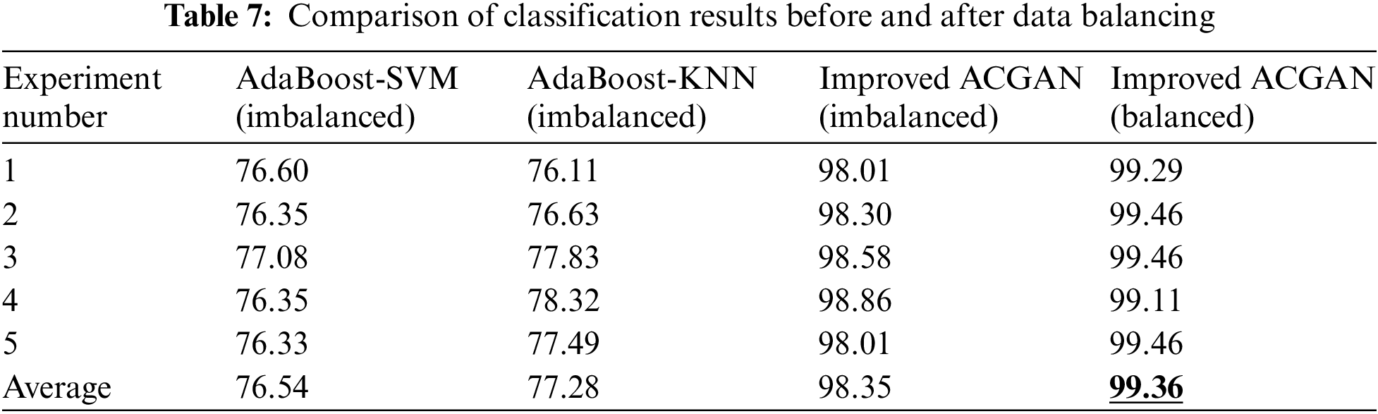
It can be seen from Table 7 that the average accuracy of Adaboost-SVM and Adaboost-KNN before data balancing is 76.54% and 77.28%, respectively, indicating that when the data set contains large categories of samples that are difficult to classify correctly, the mechanism of AdaBoost itself cannot solve the unbalanced data well. Under the improved ACGAN model, the highest fault diagnosis accuracy before DGA data balance is 98.86%, and the average accuracy is 98.35%. After DGA data balancing, the highest fault diagnosis accuracy can reach 99.46%, and the average accuracy is 99.36%, which is significantly improved compared with that before DGA data balancing.
5.2 Results and Analysis of Experiment 2
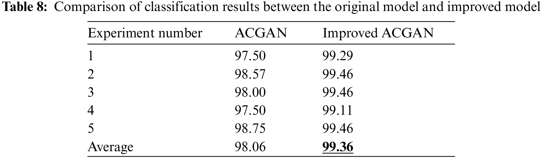
In order to verify the validity and effectiveness of the presented diagnosis model, the steps of Experiment 1 are repeated in this experiment using the balanced DGA dataset. The experimental results are shown in Table 8. Under the ACGAN model, the fault diagnosis accuracy of the transformer is 98.75%, and the average accuracy is 98.06%. Based on the improved ACGAN model, the fault diagnosis accuracy of the transformer can be improved, as described in the previous section.
The classification loss of the discriminator based on the transformer fault diagnosis model before and after ACGAN improvement is shown in Fig. 7. It can be seen from the graph that there is still certain degree of oscillation at the end of training epoch for classification loss of the fault diagnosis model based on ACGAN. While the classification loss of the fault diagnosis model based on the improved ACGAN has small overall stage fluctuation, good stability, and relatively fast convergence.
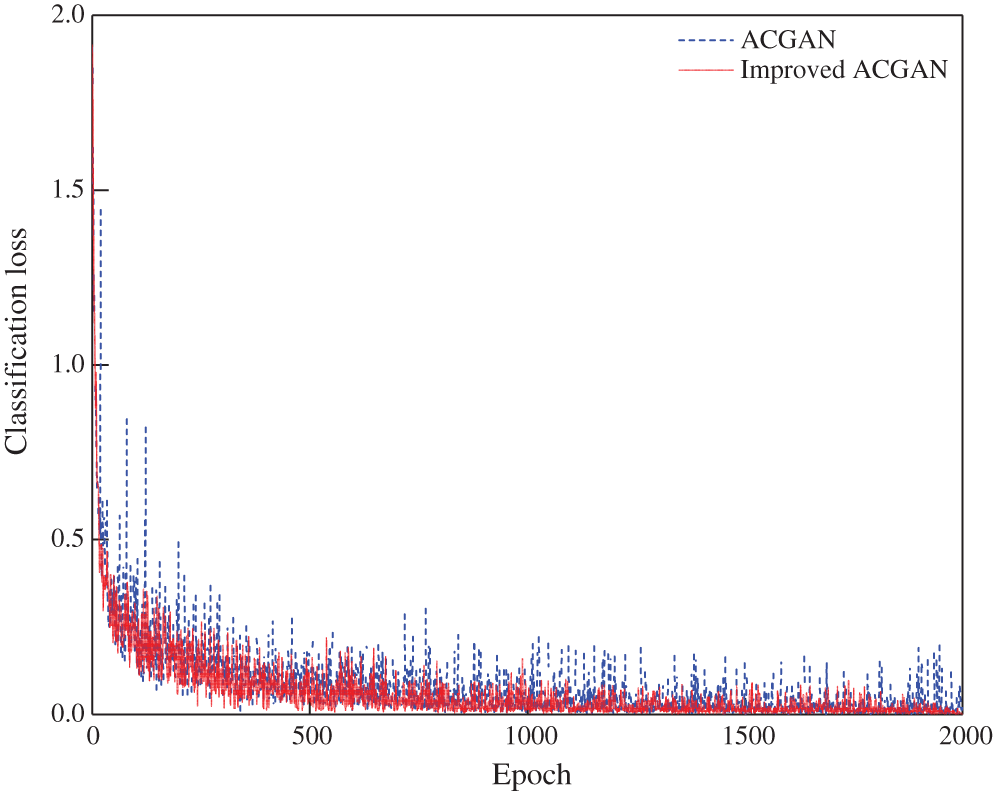
Figure 7: Comparison of classification loss results of ACGAN and improved ACGAN
5.3 Results and Analysis of Experiment 3
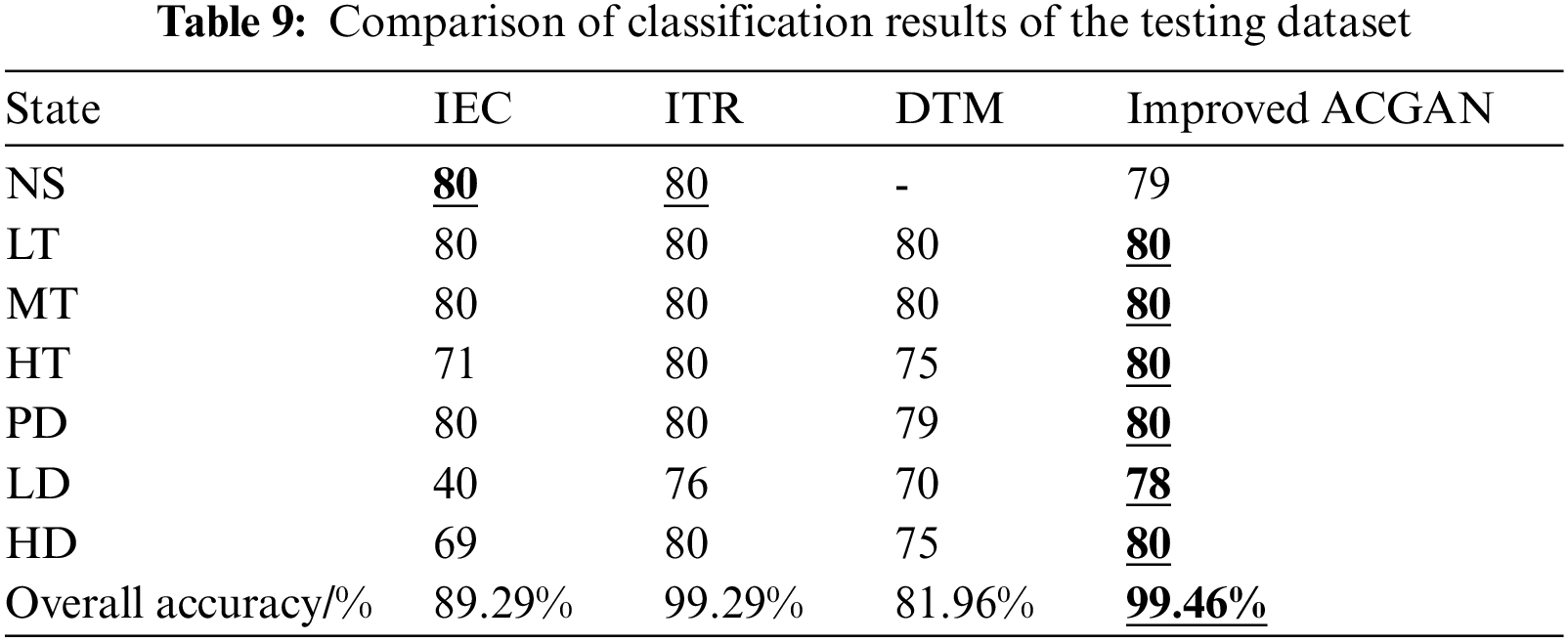
To reveal the superiority of the deep learning methods compared with conventional diagnosis methods, two groups of comparative experiments were conducted based on different traditional fault diagnosis methods under the balanced dataset, including IEC, ITR and DTM. The experimental results are shown in Table 9. The proposed method has the highest fault diagnosis accuracy (99.46%), with only three samples of discrimination errors, which verify the satisfying and remarkable diagnosis performance of the presented model.
5.4 Results and Analysis of Experiment 4
To verify the superiority of the deep learning model compared with the traditional machine learning model, this experiment implemented two different traditional machine learning-based transformer fault diagnosis models under the balanced dataset to conduct two groups of comparative experiments, including BPNN, PNN and KNN. The experimental results are shown in Figs. 8a–8d.
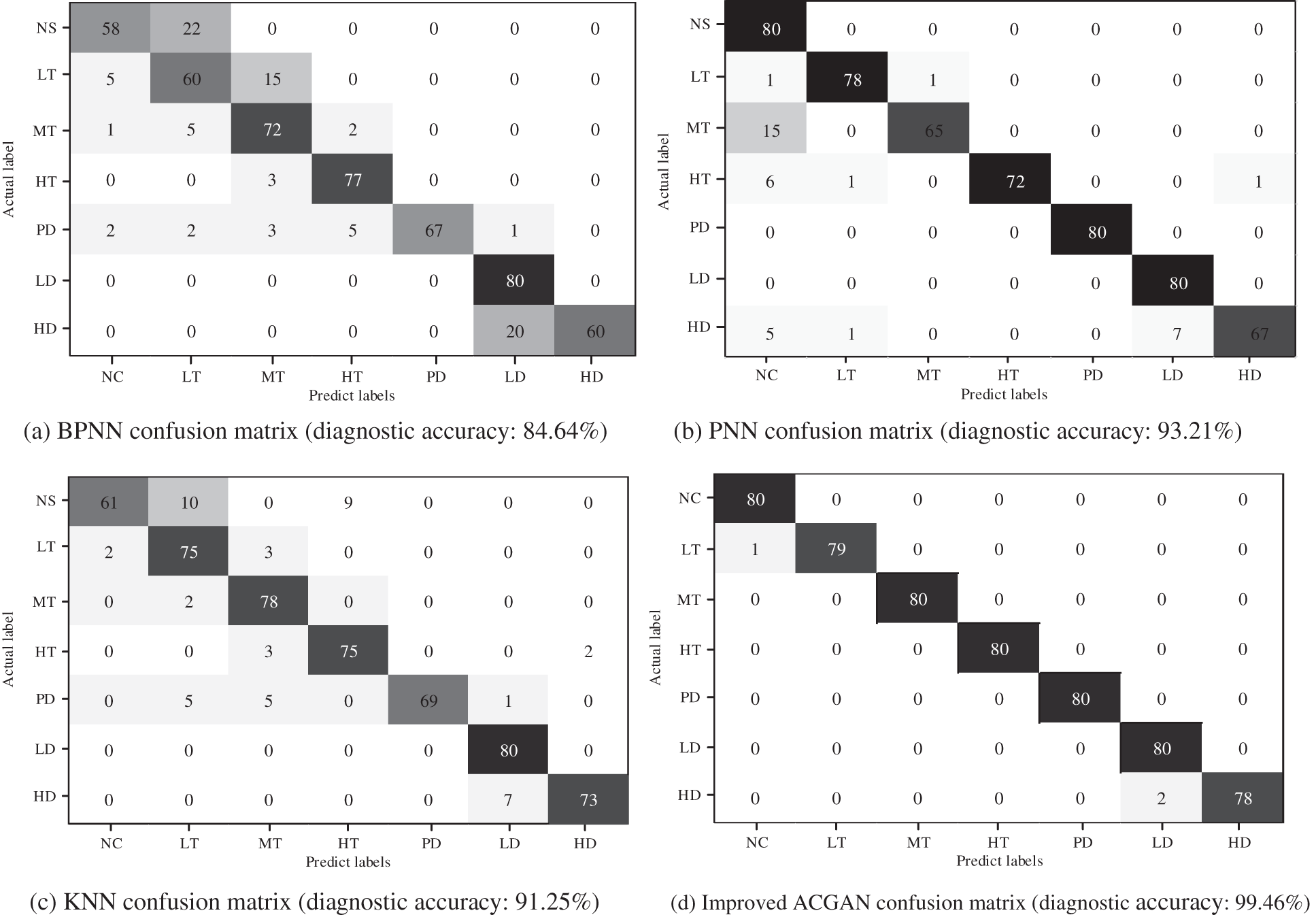
Figure 8: Comparison of confusion matrix. (a) BPNN confusion matrix (diagnostic accuracy: 84.64%), (b) PNN confusion matrix (diagnostic accuracy: 93.21%), (c) KNN confusion matrix (diagnostic accuracy: 91.25%), (d) improved ACGAN confusion matrix (diagnostic accuracy: 99.46%)
In the confusion matrix, each column represents the actual sample number of fault types, each row represents the predicted sample number of fault types, and the diagonal represents the correct sample number of fault types predicted by the model. The deeper the square color is, the higher the accuracy is. Therefore, compared with BPNN and PNN, the diagnostic accuracy of each fault type based on improved ACGAN is higher.
5.5 Results and Analysis of Experiment 5
To verify the superiority of the proposed transformer fault diagnosis model based on improved ACGAN, under the balanced DGA dataset, six kinds of transformer fault diagnosis models based on traditional deep learning are used for six groups of comparative experiments, including multilayer perceptron (MLP), convolutional neural network (CNN), long short-term memory network (LSTM), gated recursive unit (GRU), convolutional neural network-long short-term memory network (CNN-LSTM), and convolutional neural network-gated recursive unit (CNN-GRU). The model parameters are all consistent with this paper.
Since it is unreasonable to use classification accuracy only to evaluate performance of a fault diagnosis model, so other indices, including accuracy, precision, recall and F1-score, are applied in this study to estimate the generalization and classification abilities of each deep learning model more effectively and comprehensively. Let i represents the transformer fault category number, and the calculation method for each index is shown as Eqs. (7)–(10).
where, TPi represents a true positive example, indicating that the prediction is correct for positive samples. FPi denotes a false positive case, indicating that the prediction is a wrong positive sample. TNi is a true negative, indicating that the prediction is correct for the negative samples. FNi is a false negative example, indicating that the prediction is a wrong negative sample, and the sum of the four denotes the total samples.
Fig. 9 shows the accuracy, precision, recall, and F1-score of six traditional deep learning methods and the proposed method. It can be seen that the results of various indicators based on the MLP, CNN, LSTM, and GRU fault diagnosis models are unsatisfied, because the single neural network has a poor ability to extract DGA features and is difficult to extract local features effectively. Since the combination model can well mine more comprehensive feature information from the data and has better fitting ability and generalization performance, so the results of various indicators based on the CNN-LSTM and CNN-GRU fault diagnosis models are better than that of other machine learning-based methods. The proposed improved ACGAN transformer fault diagnosis method has the highest results in various indicators, which fully reflects the excellent generalization and classification abilities of the presented model.
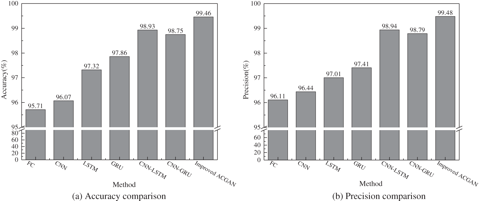
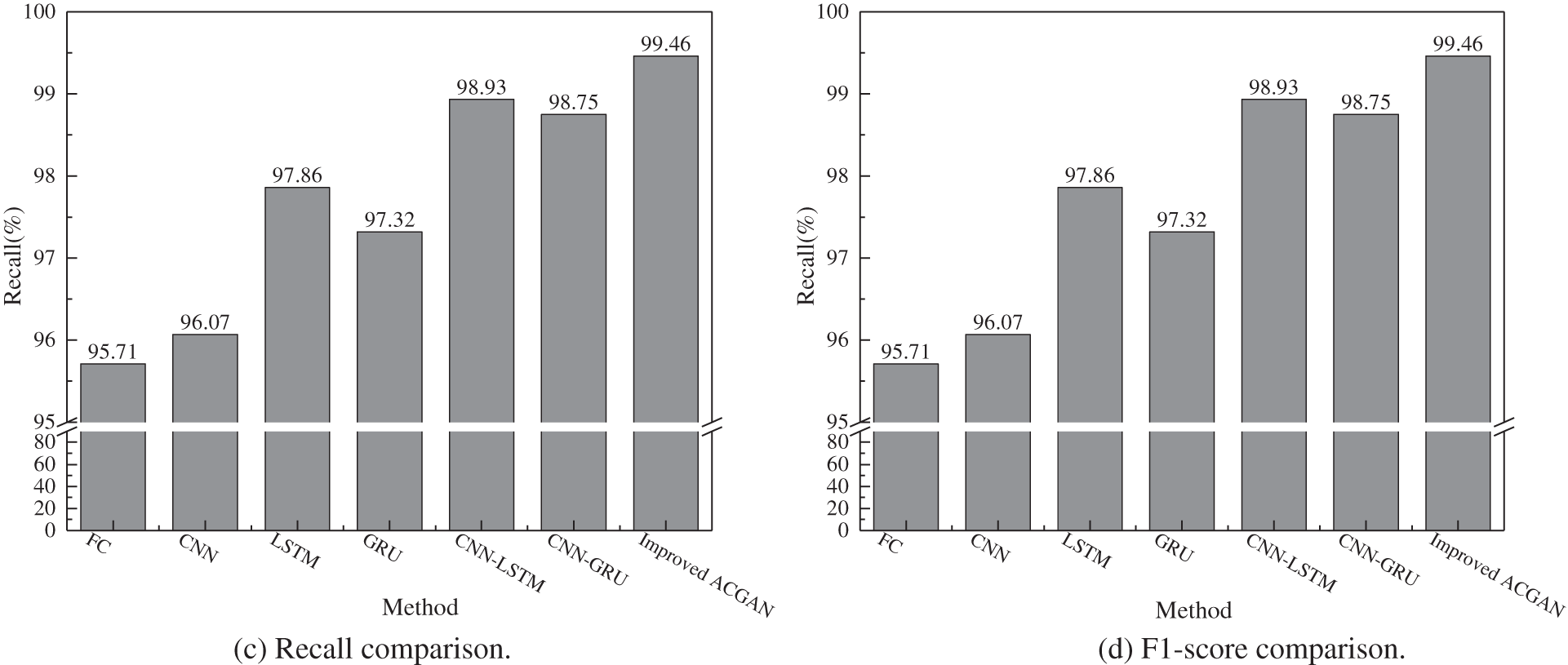
Figure 9: Comparison of the confusion matrix, (a) accuracy comparison, (b) precision comparison, (c) recall comparison, (d) F1-score comparison
5.6 Results and Analysis of Experiment 6
In order to testify the practical application of the transformer fault diagnosis model based on the improved ACGAN proposed in this paper, two actual case sample sets are used for fault classification, namely, the fault equipment database inspected in the operation of IEC TC 10 (denoted as dataset S1) [32] and the IEEE Dataport public dataset (denoted as dataset S2) [33]. The dataset S1 and dataset S2 are totally independent from the training set dataset and do not undergo any data preprocessing, which can fully reflect the actual operation of the oil-immersed transformer. The distribution of fault types for dataset S1 and dataset S2 is shown in Table 10.
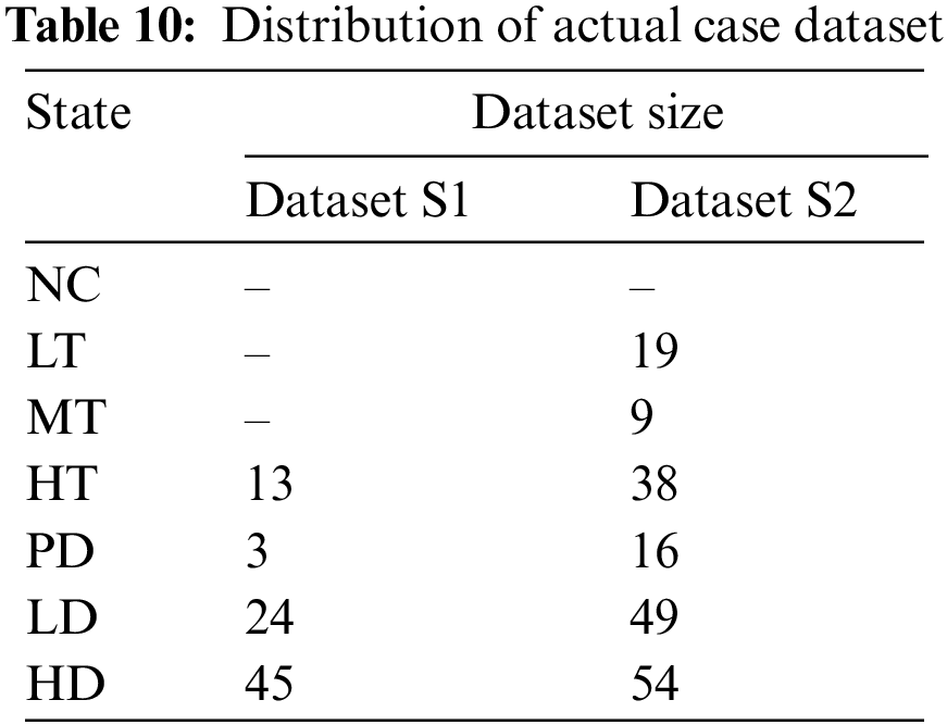
The balanced DGA dataset is used as the training dataset, and the dataset S1 and dataset S2 are used as the testing datasets for each fault diagnosis model. All diagnosis models mentioned above are used for fault diagnosis. The diagnosis results are shown in Tables 11 and 12.
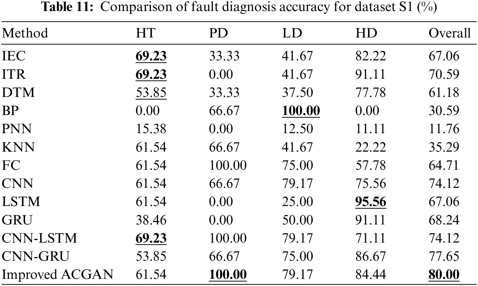
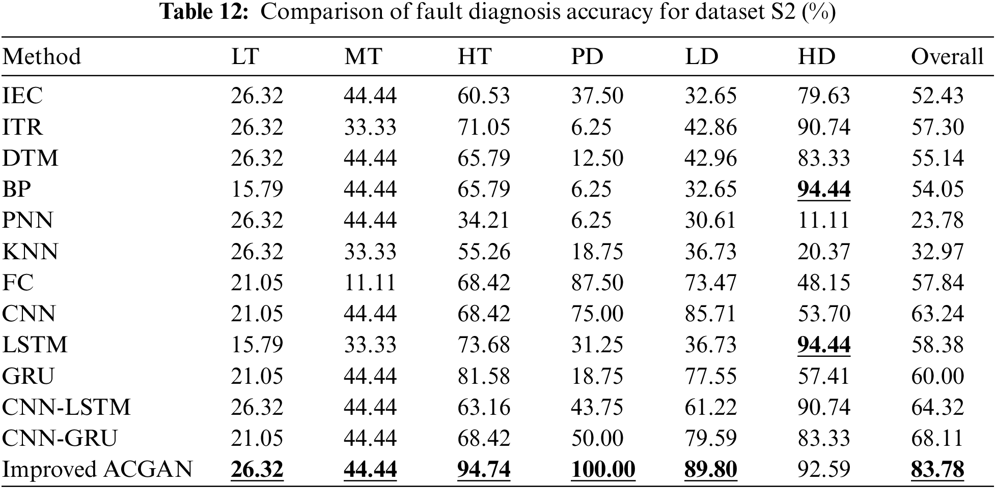
It can be seen from Tables 11 and 12 that the overall diagnostic accuracy of the fault diagnosis method based on improved ACGAN is the highest in the datasets S1 and S2, which are 80.00% and 83.78%, respectively. For specific faults, except HT, LD, and HD of dataset S1 and HD of dataset S2, the proposed method has the maximum fault diagnosis accuracy for each fault. Experiments show that the model has some practical utility.
Aiming at the adverse effects of DGA data imbalance, this paper proposes a transformer fault diagnosis method based on improved ACGAN, which is able to meet the requirements of DGA data balancing and fault diagnosing simultaneously. The effectiveness of the proposed method is verified by several comparative experiments, and the obtained conclusions are listed as follows:
(1) The generator combined models of 1D-CNN and LSTM can effectively learn the mathematical distribution, feature information of DGA data, make the generated data closer to the real data distribution and make the model more stable. While the application of MLP for the discriminator can prevent from losing significant features of DGA data when the network is too complex and has too many layers.
(2) Fault diagnosis accuracy after DGA data balance is significantly improved with the employment of improved ACGAN model.
(3) Six groups of comparative experiments are implemented to reveal the validity and superiority of the data balance and fault diagnosis performance of the proposed methods. The obtained results suggest that compared with the traditional gas concentration ratio methods, machine learning diagnosis methods and existed deep learning approaches, the critical indices of the proposed ACGAN method, including accuracy, precision, recall, and F1-score, outperform that of all other methods.
(4) Compared with other conventional methods, the proposed ACGAN method provides the best and the most satisfying fault diagnosis performance under two public DGA datasets, which verifies the availability and reliability of the proposed approaches.
(5) The proposed approach is able to offer remarkable diagnosis accuracy. However, there still exist some shortcomings that are needed to be solved in the future, including complex structures, long computing time, non-optimized parameters, limited samples and GAN models. Additionally, more indicators but DGA for fault diagnosis of power transformers, including environmental parameters, load and power, temperature, vibration signals and so on, are needed to be employed to provide more accurate and reliable results.
Funding Statement: The authors gratefully acknowledge financial support of national natural science foundation of China (No.52067021), natural science foundation of Xinjiang Uygur Autonomous Region (2022D01C35), excellent youth scientific and technological talents plan of Xinjiang (No.2019Q012) and major science & technology special project of Xinjiang Uygur Autonomous Region (2022A01002-2).
Conflicts of Interest: The authors declare that they have no conflicts of interest to report regarding the present study.
REFERENCES
1. H. R. Zhang, J. X. Sun, K. N. Hou, Q. Q. Li and H. S. Liu, “Improved information entropy weighted vague support vector machine method for transformer fault diagnosis,” High Voltage, vol. 7, no. 3, pp. 510–522, 2022. [Google Scholar]
2. Y. L. Liang, Z. Y. Zhang, K. J. Li and Y. C. Li, “New correlation features for dissolved gas analysis based transformer fault diagnosis based on the maximal information coefficient,” High Voltage, vol. 7, no. 3, pp. 302–313, 2022. [Google Scholar]
3. Y. X. Liu, B. Song, L. N. Wang, J. C. Gao and R. H. Xu, “Power transformer fault diagnosis based on dissolved gas analysis by correlation coefficient-DBSCAN,” Applied Sciences, vol. 10, no. 13, pp. 4440, 2020. [Google Scholar]
4. M. M. Islam, G. Lee and S. N. Hettiwatte, “Application of Parzen Window estimation for incipient fault diagnosis in power transformers,” High Voltage, vol. 3, no. 4, pp. 303–319, 2018. [Google Scholar]
5. T. Kari, W. S. Gao, A. Tuluhong, Y. YILihamu and Z. W. Zhang, “Mixed kernel function support vector regression with genetic algorithm for forecasting dissolved gas content in power transformers,” Energies, vol. 11, no. 9, pp. 2437, 2018. [Google Scholar]
6. T. Kari, W. S. Gao, D. B. Zhao, Z. W. Zhang, W. X. Mo et al., “An integrated method of ANFIS and Dempster-Shafer theory for fault diagnosis of power transformer,” IEEE Transactions on Dielectrics and Electrical Insulation, vol. 25, no. 1, pp. 360–371, 2018. [Google Scholar]
7. X. H. Yang, W. K. Chen, A. Y. Li, C. S. Yang, Z. H. Xie et al., “BA-PNN-based methods for power transformer fault diagnosis,” Advanced Engineering Informatics, vol. 39, pp. 178–185, 2019. [Google Scholar]
8. H. Malik, R. Sharma and S. Mishra, “Fuzzy reinforcement learning based intelligent classifier for power transformer faults,” ISA Transactions, vol. 101, pp. 390–398, 2020. [Google Scholar] [PubMed]
9. L. C. Hong, Z. H. Chen, Y. F. Wang, M. Shahidehpour and M. H. Wu, “A novel SVM-based decision framework considering feature distribution for power transformer fault diagnosis,” Energy Reports, vol. 8, no. 11, pp. 9392–9401, 2022. [Google Scholar]
10. G. E. Hinton and R. R. Salakhutdinov, “Reducing the dimensionality of data with neural networks,” Science, vol. 313, no. 5786, pp. 504–507, 2006. [Google Scholar] [PubMed]
11. J. Duan, Y. He and X. Wu, “A space hybridization theory for dealing with data insufficiency in intelligent power equipment diagnosis,” Electric Power Systems Research, vol. 199, no. 6, pp. 107363, 2021. [Google Scholar]
12. S. M. D. A. Lopes, R. A. Flauzino and R. A. C. Altafim, “Incipient fault diagnosis in power trans-formers by data-driven models with over-sampled dataset,” Electric Power Systems Research, vol. 201, no. 6, pp. 107519, 2021. [Google Scholar]
13. I. J. Goodfellow, J. P. Abadie, M. Mirza, B. Xu, D. W. Farley et al., “Generative adversarial nets,” Advances in Neural Information Processing Systems, vol. 27, pp. 2672–2680, 2014. [Google Scholar]
14. S. Nannapaneni, V. Sistla and V. Kolli, “Performance evaluation of generative adversarial networks for computer vision applications,” Ingénierie des Systèmes D Information, vol. 25, no. 1, pp. 83–92, 2020. [Google Scholar]
15. Z. Y. Jiao and F. J. Ren, “WRGAN: Improvement of RelGAN with Wasserstein loss for text generation,” Electronics, vol. 10, no. 3, pp. 275, 2021. [Google Scholar]
16. W. Y. Xie, J. Q. Zhang, J. Lei, Y. S. Li and X. P. Jia, “Self-spectral learning with GAN based spectral–spatial target detection for hyperspectral image,” Neural Networks, vol. 142, no. 8, pp. 375–387, 2021. [Google Scholar] [PubMed]
17. M. Arjovsky, S. Chintala and L. Bottou, “Wasserstein GAN,” arXiv preprint arXiv: 1701.07875, 2017. [Google Scholar]
18. M. Mirza and S. Osindero, “Conditional generative adversarial nets,” arXiv preprint arXiv: 1411.1784, 2014. [Google Scholar]
19. A. Radford, L. Metz and S. Chintala, “Unsupervised representation learning with deep convolutional generative adversarial networks,” arXiv preprint arXiv: 1511.06434, 2015. [Google Scholar]
20. Y. X. Li, H. J. Hou and M. K. Xu, “Oil chromatogram case generation method of transformer based on policy gradient and generative adversarial networks,” Electric Power Automation Equipment, vol. 40, no. 12, pp. 211–217, 2020. [Google Scholar]
21. Y. P. Liu, Z. Q. Xu and J. H. He, “Data augmentation method for power transformer fault diagnosis based on conditional Wasserstein generative adversarial network,” Power System Technology, vol. 44, no. 4, pp. 1505–1513, 2020. [Google Scholar]
22. J. Fang, F. Yang, R. Tong, Q. Yu and X. F. Dai, “Fault diagnosis of electric transformers based on infrared image processing and semi-supervised learning,” Global Energy Interconnection, vol. 4, no. 6, pp. 596–607, 2021. [Google Scholar]
23. G. S. Qian and J. Q. Liu, “Fault diagnosis based on conditional generative adversarial networks in nuclear power plants,” Annals of Nuclear Energy, vol. 176, no. 90, pp. 109267, 2022. [Google Scholar]
24. Y. Wang, G. Hug, Z. Liu and N. Zhang, “Modeling load forecast uncertainty using generative adversarial networks,” Electric Power Systems Research, vol. 189, pp. 106732, 2020. [Google Scholar]
25. A. Odena, C. Olah and J. Shlens, “Conditional image synthesis with auxiliary classifier GANs,” in Proc. of the 34th Int. Conf. on Machine Learning, Sydney, NSW, Australia, pp. 2642–2651, 2017. [Google Scholar]
26. X. C. Duan, “Research on multi-classification model and fault diagnosis of power transformer based on DGA,” Ph.D. Dissertation, Kunming University of Science and Technology, China, 2017. [Google Scholar]
27. A. Kirkbas, A. Demircal, S. Koroglu and A. Kizilkaya, “Fault diagnosis of oil-immersed power transformers using common vector approach,” Electric Power Systems Research, vol. 184, no. 1, pp. 106346, 2020. [Google Scholar]
28. E. Li, L. Wang and B. Song, “Fault diagnosis of power transformers with membership degree,” IEEE Access, vol. 7, pp. 28791–28798, 2019. [Google Scholar]
29. W. Luo, “Transformer fault diagnosis based on support vector machine and chemical reaction optimization algorithm,” Ph.D. Dissertation, Hunan University, China, 2017. [Google Scholar]
30. E. G. Osama and H. E. L. T. Salah, “Proposed three ratios technique for the interpretation of mineral oil transformers based dissolved gas analysis,” IET Generation, Transmission & Distribution, vol. 12, no. 11, pp. 2650–26621, 2018. [Google Scholar]
31. J. L. Yin, “Study on oil-immersed power transformer fault diagnosis based on relevance vector machine,” Ph.D. Dissertation, North China Electric Power University, China, 2013. [Google Scholar]
32. M. Duval and A. Depabla, “Interpretation of gas-in-oil analysis using new IEC publication 60599 and IEC TC 10 databases,” IEEE Electrical Insulation Magazine, vol. 17, no. 2, pp. 31–41, 2001. [Google Scholar]
33. E. W. Li, “Dissolved gas data in transformer oil-fault diagnosis of power transformers with membership degree,” IEEE Dataport, 2019. https://doi.org/10.21227/h8g0-8z59 [Google Scholar] [CrossRef]
Cite This Article
 Copyright © 2023 The Author(s). Published by Tech Science Press.
This work is licensed under a Creative Commons Attribution 4.0 International License , which permits unrestricted use, distribution, and reproduction in any medium, provided the original work is properly cited.
 Downloads
 Citation Tools