MFF-Net: Multimodal Feature Fusion Network for 3D Object Detection

1  Introduction

Object detection provides the basic condition for autonomous vehicles, which can offer data support for vehicle path planning and behavior decision-making. Autonomous vehicle requires accurate location and detection of obstacles in space to avoid vehicle accidents in complex traffic scenarios. Therefore, how to enable high-precision and high-efficiency object detection in different ways has attracted more and more attention from researchers. References [1–3] point out that object detection of multimodal fusion performs well in complex traffic scenarios, which can make up for the shortcomings of different information, and realize information complementation between various sensors. Therefore, it has become a research hotspot for researchers.

The existing object detection algorithms mainly include: 1) 2D object detection; 2) 3D object detection based on Light Detection and Ranging (LIDAR) point cloud; 3) 3D object detection based on multimodal fusion. Where, 2D object detection technology is mainly divided into two categories: one is an object detection algorithm based on candidate region extraction, such as Regions with Convolutional Neural Network (CNN) features (R-CNN) [4], Fast R-CNN [5], Faster R-CNN [6], etc. Transforming the object detection problem into a binary classification problem, it improves object detection accuracy through the excellent classification performance of the object detection algorithm against the data set. The other is an object detection algorithm based on regression, such as the you only look once (YOLO) series [7–9] algorithm, which integrates the object classification and localization problems in the detection into the same network for processing. Thus, training supports object classification, localization, and optimization of the network loss function. 2D object detection can make full use of rich visual information, but it is not sensitive to object distance information and cannot achieve accurate object positioning.

There are three categories of 3D object detection algorithms based on the LIDAR point cloud: the first category is to voxelized the original point cloud, convert it into voxelized data, and input it into the network for object detection; The second category is to transform the original point cloud into a 2D image through coordinate transformation and input it into the network for object detection; the third category is to directly perform feature extraction on the original point cloud and perform object detection. In [10,11], the raw point cloud is first voxelized. Then the voxelized features are learned, and finally, the 3D object bounding box is output. Pointpillars [12], first converts the original point cloud into a sparse pseudo image and then uses a 2D object detection algorithm to perform feature extraction and detection on the pseudo image and generate a regression 3D object bounding box. PointRCNN [13], first detects the original point cloud rapidly based on the predicted point cloud tag, and generates a 3D object bounding box from top to bottom. However, the information detected by the object detection algorithm of a single LIDAR sensor is too solitary to make up for its shortcomings.

There are three categories of 3D object detection algorithms based on multimodal fusion. The first category is to extract features from LIDAR point clouds and camera images, and then input them into the same network for object classification and regression, which is called pre-fusion. In pre-fusion, the modalities are interconnected to achieve a common perception through feature sharing. In AVOD [14], first inputs the original point cloud bird’s eye view (BEV) of the LIDAR and camera image, then generates the corresponding feature map through the feature extraction network and then uses region proposal network (RPN) [6] to generate candidate region. The feature map is fused according to the candidate region score, and finally, the classification and regression results are output. References [15,16] propose a continuous convolution method to fuse BEV and image features, which projects the BEV pixels into 3D space, then maps the projection points to the image features to generate the corresponding BEV image features, and finally generates a 3D bounding box by combining BEV image features with camera image features. References [17,18] supports the fusion of features by adding Squeeze-and-excitation networks (SENet) [19] to the pre-fusion network. First, the point cloud front view (FV), BEV, and image are input, and features of each channel are extracted through three feature extraction networks, then the multi-view features are input to the attention mechanism module for fusion, then different weights are assigned based on the importance of the multi-view features, and finally, the fused points are re-voxelized to generate the final object detection result. The network has good robustness, which indicates that SENet [19] addition can effectively suppress invalid features and enhance effective features.

The second category allows interaction between different feature layers based on pre-fusion to generate more accurate detection results, which is called deep fusion. In MV3D [20], as a classic deep fusion network, extracts FV, BEV, and RGB (Red, Green, and Blue) image features then uses RPN [6] to generate candidate regions for BEV and then maps the candidate regions to FV and RGB images, respectively, performs regions of interest (ROI) pooling on each view feature. The fused features are used for the classification and regression of the final fully connected layer, but when the network projects the point cloud to different views, information loss will occur and affect the detection accuracy. 3D-CVF [21] proposes a two-stage in-depth fusion method to reduce information loss. In the first stage, automatic calibration feature projection is used to convert planar features into three-dimensional spatial features, and then the two features are fused through an adaptive gated network. In the second stage, ROI is refined for the fusion features, and finally, network detection is completed. The algorithm can fuse 2D images from multiple perspectives. The network has rich fusion features and high detection accuracy. However, due to network structure limitations, compared with the end-to-end algorithm, the detection speed is slow. References [22,23] proposed a cross-modal deep feature learning framework for brain tumor segmentation tasks. Reference [22] Designed a modality-aware feature embedding mechanism to infer important weights for modal data during network learning. Reference [23] mainly consists of two learning processes: the cross-modal feature transformation process and the cross-modal feature fusion process, which aims to learn rich feature representation data and fuse knowledge from different modal data by transferring knowledge across different modalities. The proposal of these two deep fusion methods provides great potential for the application of multimodal fusion in the field of medical segmentation.

The third category is to perform object detection on the LIDAR point cloud and image separately, and fuse the output object detection results [24–26], which is known as post-fusion [27]. Introduces a new vision measurement model to visually determine the object category and shape, which enhances the data association and motion classification performance amid LIDAR point cloud and image fusion. However, in complex scenarios, visual distance is prone to big errors, resulting in decreased accuracy after fusion. References [28,29] use the CNN to fuse the features extracted from LIDAR point cloud with the image feature extraction network, apply ROI pooling to candidate regions after convolution, and finally output the classification results of 2D object detection. It achieves semantic consistency between visual classification detection and LIDAR point cloud distance detection, but 3D detection performance is not verified.

Despite certain success in the above object detection algorithms, there are still the following limitations: 1) It is difficult for a single sensor to respond to complex traffic environment perception information, cameras cannot capture accurate depth information, and LIDARs cannot access information such as color and texture. Also, the detection accuracy still needs to be further improved. 2) From the Karlsruhe Institute of Technology and Toyota Technological Institute (KITTI) [30] rankings of the open-source data set in object detection, it can be seen that most of the existing pre-fusion networks and deep-fusion networks are inherently complex and difficult to achieve real-time performance, showing unsatisfactory real-time application effects. 3) The post-fusion method, which performs object detection on different data before fusion, has relatively flexible fusion methods but is rarely studied at present. With limited applications, it is rarely applied to vehicle object detection in traffic scenarios.

In response to the above problems, under the premise of guaranteeing real-time performance in the environmental perception system, this paper proposes Multimodal Feature Fusion Network for 3D Object Detection (MFF-Net) to improve the 3D object detection accuracy and reduce the false detection rate. Specifically, the main contributions of this paper are as follows:

(1)   This paper proposes a Spatial Transform Projection (STP) method to project 2D image features to 3D point cloud BEV features.

(2)   An Adaptive Expressive Enhancement (AEE) fusion network is constructed to focus on important features and suppress unnecessary features.

(3)   An adaptive non-maximum suppression (A-NMS) algorithm with better performance is proposed.

(4)   Extensive experiments on large-scale datasets KITTI [30] and nuTonomy scenes (nuScenes) [31] show that the method has high detection efficiency and accurate detection performance.

2  Methodology

This paper aims to build a multi-modal fusion 3D vehicle object detection network with good real-time performance and high accuracy. 3D-CVF [21] is selected as the backbone network. Space Transformation Projection (STP) algorithm, Adaptive Expressiveness Enhancement (AEE) fusion network, and Adaptive Non-Maximum Suppression (A-NMS) bounding box removal method are taken for network improvement.

The improved network structure is shown in Fig. 1. First, 2D image and 3D point cloud are input into respective feature extraction networks to extract camera image features and LIDAR point cloud features. Because of the different features and distribution characteristics of camera images and LIDAR point clouds, Using the STP algorithm to map camera image features to camera BEV features with a high degree of correspondence with LIDAR point cloud BEV features. Then, the camera BEV feature and LIDAR BEV feature are cascaded and input into the AEE fusion network with the ability to improve feature directivity. According to the channel attention mechanism SENet [19], each feature channel is assigned different weights based on its importance to enhance the important features of each channel in the cascaded LIDAR-Camera, while useless features are suppressed. Then, the cascaded LIDAR-Camera fusion features are input to the detection output network. Here, the region proposal network (RPN) [6] is first used to generate the corresponding region of interest (ROI) box on the cascade feature, which is then input to the 3D fusion network of interest for further fusion. The image plus the shallow features of the LIDAR point cloud is also an input for better fusion accuracy. For Convolutional Neural Networks (CNN), different depths correspond to different levels of semantic features. Shallow networks with high resolution learn more detailed features; deep networks with low resolution learn more semantic features and lose location information. Accordingly, by combining shallow features and deep features, shortcomings in the separate processing of the two can be compensated. Finally, the A-NMS algorithm is used to filter out an unimportant bounding boxes and perform 3D object detection at the same time.

Figure 1: Overview of the proposed MFF-Net method. After each backbone network process, the point cloud and the image respectively, the spatial sransform projection (STP) algorithm is used to convert the image features into the features in the BEV. Then, the camera and LiDAR features are fused using the adaptive expressive enhancement (AEE) fusion network. Finally, the fusion network based on RoI pooling (It can generate fixed-size feature maps from LIDAR feature maps and image feature maps) is used to predict the detection output network after the scheme is refined. See Figs. 2 and 5 for more description of the involved STP algorithm and AEE fusion network

Figure 2: STP algorithm: First, given the object pixel points on the point cloud BEV, extract the K nearest LIDAR points (step 1); Then, project the 3D points onto the camera image plane (step 2); Retrieve the corresponding image features (step 3); Finally, this paper feed the image features and continuous geometric offset into the BP neural network to generate the features of the object pixel (step 4)

2.1 Space Transformation Projection (STP) Algorithm

Given, because of the inconsistent feature space in multi-modal fusion, this paper combines matrix transformation with Back Propagation (BP) neural network [32] to solve the problem that the feature map is differently expressed in the camera coordinate system and the world coordinate system during camera image and LIDAR point cloud fusion. This algorithm can guarantee that the two different features are fused without losing information, thus improving 3D object detection accuracy. MV3D [20] projects point cloud data to a two-dimensional plane from a specific perspective and then fuses data from different visual angles to complete the cognitive task. This method will lose geometric structure information and accuracy when projecting from a BEV perspective, and the final experiment results suggest that MV3D [20] is relatively applicable to large objects. However, this method does not make full use of the 3D spatial information of the point cloud, and it is still difficult to accurately detect objects with rich local features.

To further cope with the problem that the data information collected by the camera and the LIDAR sensor in the multi-modal fusion has different space feature distribution. This paper proposes the STP algorithm, as shown in Fig. 2. The STP algorithm is composed of space transformation projection and BP neural network model.

The main idea of deep parametric continuous convolution [33] is to use a multilayer perceptron as the parameterized kernel function of the continuous convolution, and the parameter kernel function connects the entire continuous domain. Whereas, the costly continuous convolution can be weighted over a limited number of adjacent points. According to the different weights of each adjacent object and its relative geometric offset from the object, the parameter continuous convolution formula is as follows:

hj=∑jMLP(xi−xj)⋅fj(1)

where j indexes the neighborhood of the point i, fj is the input feature, and xj is the continuous coordinate associated with the point. The Multilayer Perceptron (MLP) computes the convolution weights for each adjacent point.

The STP algorithm proposed in this paper first exploits the input camera image feature map and a set of LIDAR points. The goal of the STP algorithm is to build a dense BEV feature map, where each discrete pixel contains features generated from the camera image. Then, this dense feature map can be easily fused with the BEV feature map extracted from LIDAR. One difficulty with image BEV fusion is that not all discrete pixels on the BEV space are observable in the camera. To solve this problem, each object pixel in the dense map uses Euclidean distance on the 2D BEV plane to find its closest LIDAR points. Finally, this paper utilizes a BP neural network to fuse the information from these K closest points (in the experiment, setting the value of K to 10.) to insert the unobserved features of the object pixel. The input of the BP neural network consists of two parts: first, the corresponding image features are extracted by projecting the raw LIDAR points onto the image plane. Bilinear interpolation is used to obtain image features at consecutive coordinates.

The 3D neighbor offsets between original LIDAR points and object pixels are encoded on a dense BEV feature map to model LIDAR point dependencies. Overall, each object pixel provides input to the BP neural network [32]. For each object pixel, the BP neural network outputs feature by summing the BP neural network outputs of all adjacent pixels. The formula is as follows:

hi=∑jBP(concat[fj,xj−xi])(2)

where fj is the input image feature for the point j, xj−xi are the 3D offsets from neighboring point j to an object i, and concat(⋅) is the concatenation of multiple vectors. In practice, this paper uses a 3-layer perceptron, where each layer has hidden features.

The STP algorithm can solve the problem of inconsistency between image and point cloud feature space, and further, enrich the network feature information by splicing and fusion in the feature mapping channel. Mapping image and point cloud features to the same spatial features is expected to further improve the accuracy of the network.

2.2 Adaptive Expressiveness Enhancement (AEE) Fusion Network

In practical object detection scenarios, existing networks sometimes fail to focus on or miss important object features. To this end, based on the STP algorithm designed in Section 2.1, In this paper, an Adaptive Expressive Enhancement (AEE) fusion network is adopted to enhance the expressive power of different features, focusing on important features while suppressing unnecessary features. The specific process is shown in Fig. 5. Because the squeeze-and-excitation (SE) module proposed in Squeeze-and-excitation networks (SENet) [19] is often used for feature extraction in the image domain, this paper explores the application of the attention mechanism in the SE module for multimodal fusion, and Constructed the AEE fusion network. The SE module is shown in Fig. 3.

Figure 3: Schematic diagram of SE module: In the Fig., Fsq (‘•’) represents the squeeze operation, Fex (•, W) represents the excitation operation, and Fscale (‘•’) represents the feature recalibration

The SE module in Fig. 3 processes the feature map derived from the convolution and obtains a one-dimensional vector equal to the number of channels as the evaluation score for each channel. Then, the score is assigned to the corresponding channel to derive the output result. According to Fig. 3, the attention mechanism is specifically implemented as follows: Given an input X, its number of feature channels is C1. After a series of convolution transformations, a feature with C feature channels is obtained. Finally, three operations are performed to recalibrate the features obtained earlier.

The specific implementation process of the AEE fusion network is shown in Fig. 4. The input feature layer size is H × W × C. In the squeeze operation, through the Max Pooling operation, the candidate size becomes 1 × 1. In the excitation operation, the first fully connected layer is used to reduce the number of channels too C/r, r is the zoom factor used to reduce the number of channels and thereby the amount of calculation. In this paper, a large number of experiments prove that the effect is optimal when r=16. If the ReLU activation function is used, the feature dimension remains unchanged. The second fully connected layer is used for dimensionality, and the number of channels is changed back to C; the Sigmoid function is used to output the weight of each channel; Finally, its feature recalibration is used to multiply the weight with the original corresponding channel to obtain the weighted feature layer.

Figure 4: SE module implementation process

In summary, the AEE fusion network formed by adding the SE module is shown in Fig. 5. The AEE fusion network firstly cascades the point cloud BEV features extracted by the feature extraction network and the image features after STP algorithm to obtain the cascaded LIDAR-Camera features; then through the weighting operation of AEE fusion network, the LIDAR-Camera fusion features with different weights are output. Experiments in this paper indicate that the number of features is the highest when the number of channels C is 96. At this time, adding the SE module can get the largest feature layer receptive field, which helps to output fusion features with different weights. Based on abundant experiments, the SE module parameter reduction has the optimal effect when it is set to 16.

Figure 5: AEE fusion network architecture. First, this paper concatenates camera features and lidar features to obtain concatenated LIDAR-camera features. Then, this paper feeds the obtained cascaded features into the AEE fusion networks for operations such as squeezing, max-pooling, excitation, and feature recalibration. Finally, LIDAR-camera fusion features with different weights are output

2.3 Adaptive Non-Maximum Suppression (A-NMS) Algorithm

To further improve the accuracy of the object detection algorithm for the entire fusion network, it is necessary to delete a large number of overlapping boxes generated by RPN. Therefore, based on the AEE fusion network designed in Section 2.2, this paper further optimizes the network by adding the A-NMS module.

Non-Maximum Suppression (NMS) [34] is a commonly used method for determining candidate regions in object detection tasks. First, it ranks all bounding boxes according to their scores. The bounding box with the highest score is selected, and all other bounding boxes that significantly overlap with the bounding box with the highest score are suppressed using a predefined threshold. This process is recursively applied to the remaining bounding boxes and computes the Intersection over Union (IOU) with other candidate regions, where IOU is the ratio of the intersection and union between the Predicted box and the True box. When the IOU is greater than a certain threshold, it is suppressed to achieve the purpose of determining the optimal candidate area. The formula of the NMS algorithm is as follows:

Si={si,IoU(M,bi)<Nt0,IoU(M,bi)≥Nt(3)

where Si is the score of the candidate region after comparative calculation, si is the initial score of the candidate region, M is the candidate region with the highest score, bi is the current candidate region, IoU(M,bi) is the IOU between M and bi, Nt is the set threshold.

Through the NMS [34] algorithm, candidate regions in the image that is more in line with the actual object location and size are preserved. However, in 3D object detection, multiple objects in the image may have varying degrees of occlusion. When handling candidate regions in this case, the candidate regions of multiple objects will be suppressed due to the excessive IOU. As a result, some objects may be missed. To solve this problem, Soft-NMS [35] based on [34] attenuates the detection scores of all other objects into a weight-penalized continuous function that overlaps the bounding box with the maximum score. The calculation formula is as follows:

Si={si,IoU(M,bi)<Ntsi×(1−IoU(M,bi)),IoU(M,bi)≥Nt(4)

Although Soft-NMS [35] algorithm reduces missed detection of the NMS [34] algorithm in multi-object detection, there are still some shortcomings. In actual application, there is a gradually increasing probability of repeated detection and object misclassification in the Soft-NMS algorithm.

Aiming at the problems of Soft-NMS [35], this paper proposes an Adaptive Non-Maximum Suppression (A-NMS) algorithm. The A-NMS algorithm adds a one-dimensional threshold Ni based on the Soft-NMS algorithm, and Nt<Ni. If the intersection ratio between the candidate region bi and the highest scoring candidate region M is IoU(M,bi)>Ni, it is directly suppressed; if Nt≤IoU(M,bi)≤Ni, a penalty is given to the candidate region. The weight of the rate is combined with the original score as a penalty factor; if IoU(M,bi)<Nt, it means that the overlap area between bi and M is small, no suppression is required, keeping the original score. The mathematical expression of the A-NMS algorithm is as follows:

Si={si,IoU(M,bi)<Ntsi×(1−IoU(M,bi)),Nt<IoU(M,bi)<Ni0,IoU(M,bi)>Ni(5)

The A-NMS algorithm proposed in this paper combines the advantages of NMS [34] and Soft-NMS [35] algorithms and adds a one-dimensional threshold. This two-dimensional threshold method can reduce the probability of missed and false detection of objects in the candidate region where IoU(M,bi) is smaller than Ni.

So far, this paper has successfully constructed Multimodal Feature Fusion Network for 3D object detection (MFF-Net). Specifically, the STP algorithm is first embedded after the image feature extraction network, so that the features extracted by the image feature extraction network and the point cloud features are better fused; Then, an AEE fusion network is embedded after the LIDAR-camera cascade feature, so that the network pays more attention to the important features of the object; Finally, the A-NMS algorithm is used to remove a large number of overlapping bounding boxes to improve the detection accuracy of the 3D object of the overall network.

2.4 Network Loss Function

The loss function of MFF-Net in this paper consists of two parts: The first part is the loss function between the 3D candidate box and the ground-truth box generated by the region proposal network (RPN), and the second part is the detection loss function of the output network. The mathematical expression is as follows:

Lloss=Lcls−rpn+Lloc−rpn+Lcls−pre+Lloc−pre(6)

where Lcls−rpn represents the classification error of the RPN, Lloc−rpn represents the position regression error of the RPN, Lcls−pre represents the classification prediction error of the final network output, and Lloc−pre represents the position regression error of the final network output.

Object detection classification error: The classification task is to classify the objects in the area and determine whether it is an object, which involves a binary classification problem. Therefore, this paper selects the sparse SoftMax [36] and cross-entropy function [37] commonly used in binary classification as the error calculation function in the classification task. In this paper, two parts demand classification: the RPN part and the detection output part. The error functions of the two are the same. The loss function calculation process includes two parts: (1) SoftMax calculation of the input, with calculation formula shown in (7), which is responsible for normalizing the input classification results; (2) cross-entropy loss calculation, as shown in formula (8).

Si=eai∑i−1neai(7)

Lcls=−∑i−1n⁡yilog⁡Si(8)

where ai is the predicted classification score, yi is the true value of the label, and eai is the exponential function value of the predicted score.

Object detection coordinates regression error: The RPN predicts the difference (dx,dy,dz,dw,dl,dh) between the label truth box and the initial position box, which respectively represents the difference between the predicted label, the initial position box center coordinate, and the length, width, and height. At this time, the regression calculation box is the calculated real difference (dx∗,dy∗,dz∗,dw∗,dl∗,dh∗) between the initial position box and the label, which is expressed as the real coordinate and size difference between the initial position box and the label. The relationship between the initial position box and the label truth box is shown in Fig. 6.

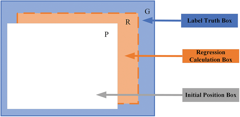
Figure 6: The relationship between the initial position box and the label truth box

The initial box is a candidate box with different sizes generated by the RPN at each pixel position of the feature map using the convolution kernel. The regression calculation box is the box position after regression calculation of the predicted (dx,dy,dz,dw,dl,dh) on the initial box and the label truth box is the object position information in the label.

The position of the final detection output part of the network regresses to the eight-point coordinates of the 3D box, and the label at this time indicates the eight-point coordinates of the 3D candidate box obtained after calculation based on the first prediction.

Both the two-position regression parts use smoothL1 the function [38] as the error term, and the formula is as follows:

Lloc=∑smoothL1(Locpre−Gt)(9)

where Locpre indicates the predicted value, Gt indicates the label information, and the smoothL1 function calculation is shown as follows:

smoothL1={0.5x2,|x|<1|x|−0.5,otherwise(10)

3  Experiment

To verify the effectiveness of MFF-Net, experimental evaluations are performed based on the Karlsruhe Institute of Technology and Toyota Technological Institute (KITTI) [30] and nuTonomy scenes (nuScenes) [31] datasets.

3.1 Experimental Environment

The experimental environment of this paper is shown in Table 1.

3.2 KITTI DataSet

The training, validation set, and testing of the network are based on the KITTI [30] dataset. The collection platform of this dataset consists of 2 gray-scale images, 2 color cameras, 1 LIDAR, 4 optical lenses, and a GPS navigation system to provide multiple sensor data. In the object detection dataset, there are a total of 14,999 data, of which 7,481 data are divided into training sets and the rest are divided into test sets. Considering that the data in the test set has no published label files. To complete the network model effect evaluation, the training set with label files is divided according to the unified classification standard of the KITTI dataset. According to the ratio of 1:1, 3471 pieces of data in the scenario data of 7481 training sets are divided into training sets, and the rest are used as validation sets for the evaluation of model data. In the network evaluation stage, the KITTI dataset officially divides the network evaluation indexes into three levels: Easy, Moderate, and Hard according to the degree of object occlusion and truncation.

3.3 nuScenes DataSet

The nuTonomy scenes (nuScenes) [31] dataset is the first large-scale multi-scene 3D object detection dataset to provide a full set of sensor data for autonomous vehicles, with more than 1000 scenes collected in two cities, Singapore and Boston. The data collected in this dataset includes 6 multi-view cameras, 32-line LiDAR, 5 mmWave radars, and GPS and IMU. It provides object annotation results within 360 degrees of the desired 10 classes of objects. Compared to the KITTI [30] dataset, it contains more than 7 times more object annotations. The dataset consists of a training set of 28,130 frames, a validation set of 6019 frames, and a test set of 6008 frames. This paper follows the official dataset split [31], using 28130 frames, 6019 frames, and 150 frames for training, validation, and testing, respectively.

3.4 2D and 3D Feature Extraction Network Details

In the image feature extraction network, this paper uses MobileNetv2 [39] as the basic convolutional layer. To prevent the network from training the network parameters of the image feature extractor in the beginning, the model uses the first few layers of parameters of the already trained MobileNetv2 as the initial convolution kernel value of the image feature extractor to save training time. The network uses the stochastic gradient descent method as the optimization function to guide the network training toward the descent direction of the loss function.

In the LIDAR point cloud feature extraction network, the predecessors often used projection, mathematical statistics, and direct convolution to preprocess the point cloud data. However, the projection method will cause original data information loss. The PointNet [40] with a 1 × 3 convolution kernel only uses about a thousand points in actual training, which is unsuitable for object detection in a traffic environment. Therefore, this paper does not use the above two methods for point cloud preprocessing but designs the input feature learning layer of the point cloud according to the PointNet direct coordinate convolution. The original data coordinate information is calculated to derive the input feature map. Then, Convolutional Neural Network (CNN) is used to complete the feature extraction of the point cloud.

The point cloud feature extraction network first uses three-dimensional convolution to perform three 3D convolutions on the input 10 × 400 × 352 × 128 sparse feature data. The feature map with a height of 10 is down-sampled three times to obtain a 2 × 400 × 352 × 64 feature map. Then, the feature map is reshaped to transform into a 400 × 352 × 128 two-dimensional multi-channel feature map. Finally, using 2D convolution and deconvolution operations, down-sampling is performed by 8 times and then up-sampling by 4 times to output a feature map with a resolution of 200 × 176 × 512.

3.5 Evaluation Index

The evaluation indexes are the general 3D object detection evaluation index: Precision (P), Recall rate (R), Average Precision (AP), and mean Average Precision (mAP):

P=TPTP+FP(11)

R=TPTP+FN(12)

where True Positive (TP) represents a truly positive example, False Positive (FP) represents a false positive example, and False Negative (FN) represents a false negative example.

In this paper, the R is divided into 11 points (0.0, 0.1, 0.2…, 1.0). To evaluate the network model from several aspects, the average accuracy rate is generally selected as the judgment index in the object detection task. The AP in the object detection task has a different definition from conventional mathematical statistics. In the network model, the recall rate is the abscissa and the accuracy is the ordinate, and the Precision-Recall (P-R) curve can be drawn. The area enclosed by the P-R curve and the coordinate axis is the AP value.

On the validation set, this paper makes statistics of the predicted value and the actual true value. When setting different classification thresholds, the bounding box IOU and the classification score threshold are used as variables to calculate the R and accuracy of the validation set. The P-R curve of the model is plotted on the validation set to calculate the network AP. The trained network model is used to predict the divided validation set and based on the predicted output classification scores and bounding box coordinates, the predicted results are compared to the labels using the evaluation algorithm. Different IOU thresholds are set to calculate TP, FP, and FN under different thresholds, and plot the recall and accuracy of 2D and 3D object detection on the P-R coordinate system. The results are shown in Fig. 7.

Figure 7: P-R Curve. (a–c) are the 3D P-R curves of the 3D object detection results of the KITTI validation set of cars, pedestrians, and cyclists, respectively. (d–f) are the P-R curves of 2D object detection after projecting the 3D bounding box to the 2D bounding box

The Easy, Moderate, and Hard in Fig. 7 are divided according to the size of the pixel value occupied by the object and the degree of occlusion. The area enclosed by the P-R curve is calculated to obtain the average network accuracy. As shown in Table 2, which includes the average accuracy of 2D and 3D object detection.

3.6 Network Training Parameters

On the KITTI [30] dataset, the MFF-Net training parameters are set as follows: Mini-batch is used in the training set to reduce the calculation amount, and the batch size is set to 6. 0.00256 is used as the initial network learning rate on the training set. The learning rate of the 800th generation and the 850th generation is reduced to 0.1 times of the original, to avoid the large learning rate of the network in the later stage, which leads to the loss of excessive vibration during training, and the slow convergence speed of the network in the later stage. To ensure the fairness of the comparative experiments, the training parameters of the baseline network 3D-CVF [21] and the addition of the STP algorithm and AEE fusion network are consistent with the training parameters of the MFF-Net network. In the RPN stage, since a large number of regions in a traffic scenario belong to the background, far more negative samples are generated than positive samples. Therefore, in the candidate region stage, the network performs batch processing and selects 128 samples at a time. The positive and negative samples are selected at a ratio of 1:3 as the input of the second-stage network. For the nuScenes [31] dataset, this paper uses the same learning rate as in the KITTI dataset to train the network, and the batch size is set to 2. Due to the class imbalance problem in the nuScenes dataset, this paper adopts the method of DS sampling [41] to alleviate this problem.

3.7 KITTI Test Results and Analysis

To verify the effectiveness of the STP algorithm, AEE fusion network, and A-NMS algorithm, the ablation experiment are designed for different network modules and all ablation experiments are implemented based on the KITTI [30] data set.

Table 3 shows the object test results of the original baseline 3D-CVF [21] network, STP algorithm, AEE fusion network, and A-NMS algorithm on the KITTI validation set. A detailed comparison is made on the performance of each network, including network detection accuracy and speed. The test data is specifically analyzed as follows:

(1)   As shown in Table 3, the average detection accuracy (mAP) of the STP algorithm on the KITTI dataset is 80.32%, which is 0.3% higher than the baseline network 3D-CVF. The STP algorithm changes the cross-projection transformation method of the baseline network 3D-CVF and integrates the STP algorithm. The experimental data confirm that the STP algorithm transforms the 2D image feature into a point cloud BEV feature. This method enables better correspondence between the two features, which can improve the accuracy of object detection. At the same time, compared with 3D-CVF, the detection speed after adding the STP algorithm is only reduced by about 0.8 ms, and the network still has a faster detection speed. The experimental results show that the STP algorithm only increases a small amount of computation while improving the detection accuracy of 3D-CVF.

(2)   It can be seen from Table 3 that the simultaneous addition of the STP algorithm and the AEE fusion network reflects the attention to important features and the suppression of unnecessary features. The average accuracy of 3D object detection on the KITTI dataset is 81.72%, which is higher than that of only adding the STP algorithm. With an increase of 1.4%, the detection speed is only reduced by about 0.5 ms, and real-time detection can still be guaranteed.

(3)   To remove a large number of unnecessary overlapping bounding boxes extracted by the RPN during the 3D object detection, this paper proposes MFF-Net, which has an average 3D object detection accuracy of 82.60% on the KITTI dataset. Compared with the 3D-CVF baseline model, the performance improves by 2.58%.

The above experimental results show that the modules added in this network design can learn the correlation between channels and screen out the attention for the channels. Although the calculation amount is slightly increased, it does not affect the real-time detection, and the obtained results are obtained. With relatively high detection accuracy, with the development of network hardware, the real-time performance will be further improved.

Table 4 shows the experimental comparison between the baseline network and the 3D object detection networks currently popular in the various KITTI dataset lists. In single-modal detection, this paper selected VoxelNet [10], PointRCNN [13], SECOND [42], PointPillars [12], and STD [43] networks; In multimodal fusion network, this paper selected PointPainting [2], MV3D [20], AVOD [14], F-PointNet [44] and 3D-CVF [21] networks. According to Table 4, The MFF-Net network proposed in this paper has obvious advantages compared with other networks. Although it is slower than some networks in detection speed, it achieves an average accuracy of 90.96%, 80.97%, and 75.39% on the three important evaluation indicators Easy, Moderate, and Hard. Compared with the average accuracy of the baseline 3D-CVF network on the Easy, Moderate, and Hard evaluation metrics, the accuracy of MFF-Net is improved by 2.27%, 2.81%, and 2.66%, respectively.

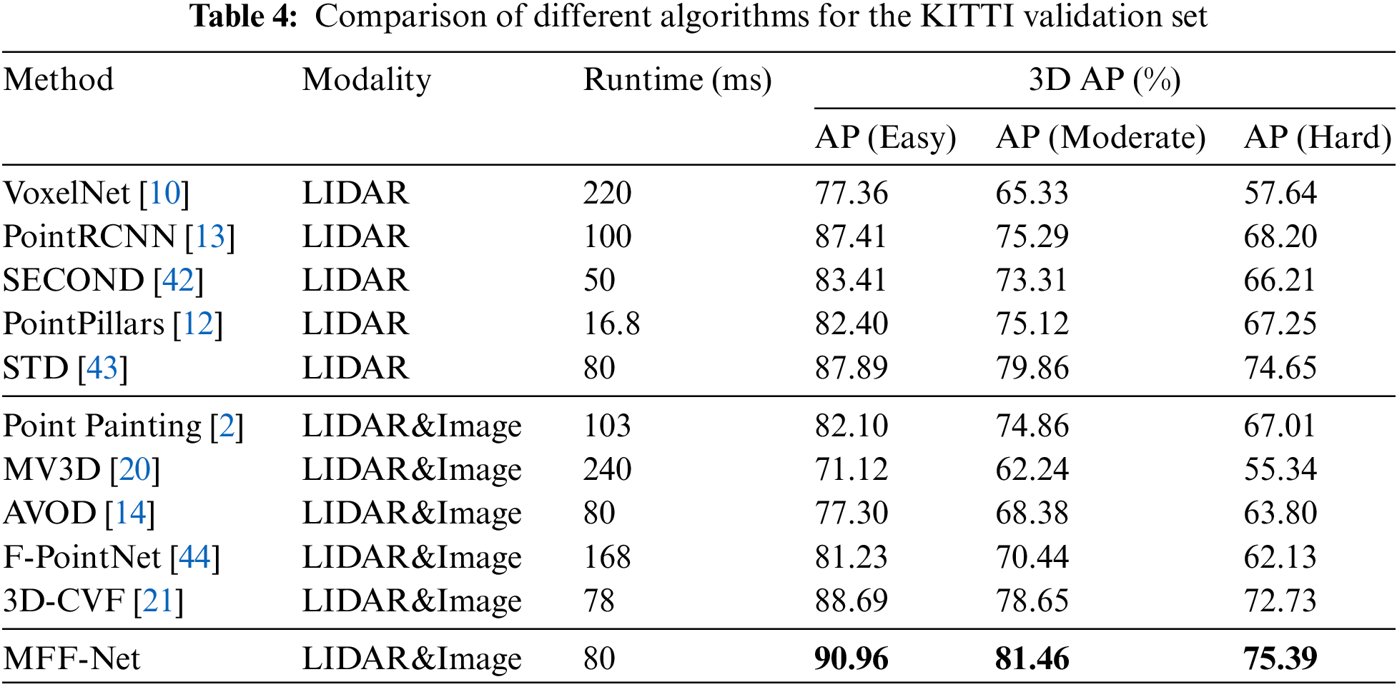
Table 5 presents an experimental comparison between MFF-Net and the 2D object detection accuracy measured on the KITTI [30] dataset using you only look once (YOLO) V4 [45] and YOLO V5 [46]. As can be seen in Table 5, the MFF-Net network has clear advantages over other 2D object detection networks. Although the detection speed is slower than that of the YOLO V4 [45] and YOLO V5 [46] networks, the MFF-Net network achieves 94.67%, 91.36%, and 84.11% average accuracies on three important evaluation metrics, respectively. The average accuracy in the Easy, Moderate, and Hard evaluation indicators is higher than that of YOLO V4 [45] and YOLO V5 [46].

3.8 nuScenes Test Results and Analysis

This paper also tests MFF-Net on the nuScenes [31] dataset to validate the performance obtained by multimodal fusion. To this end, this paper compares the proposed MFF-Net network with a baseline network whose structure is the same as MFF-Net, except that the camera results are not used. For the fairness of the comparison, this paper also applies the DS sampling strategy to the baseline network. To compare the experimental results, this paper also adds the performance of Second [42], PointPillar [12], PMPNet [47], CVCNet [48], and HotSpotNet [49]. Table 6 also provides the average precision AP of 10 classes, mAP, and nuScenes detection score (NDS) implemented by several other popular 3D object detection networks at this stage. As can be seen from Table 6, in the metrics of mAP and NDS, the performance of MFF-Net is improved by 5.5% and 6.2% over the baseline network in terms of mAP and NDS evaluation metrics, respectively. The method proposed in this paper consistently outperforms baseline networks in terms of AP for all classes. Compared with other methods in Table 6, MMF-Net also shows better performance.

It should be noted that the STP algorithm designed in this paper can make the obtained BEV image features closer to the point cloud BEV features. By using the AEE fusion network, each feature channel is given a different weight to increase the important model features and suppress unimportant features, thereby enhancing feature directivity. In particular, when identifying some occluded and truncated vehicle objects, it can fully extract insignificant features for judgment, which greatly reduces the missed detection rate in vehicle detection. By adding the A-NMS algorithm and optimizing the Soft-NMS [32] algorithm, the 3D object bounding box is more accurate, which increases the probability of false detection of occluded and truncated vehicles. The above experiments reveal that the built MFF-Net network can effectively improve the network detection accuracy while still maintaining the real-time detection speed. Therefore, the network is more suitable for 3D object detection in the autonomous driving scenario.

The visual test results of this algorithm are shown in Figs. 8∼12. The KITTI validation set images and point cloud data are selected to test the vehicle object detection effect of the MFF-Net network in different complex scenarios. The following is the demonstration and analysis of missed and false vehicle object detection result under different illumination, different degrees of occlusion, and different detection distances.

Figure 8: Test results under different lighting conditions

Fig. 8 shows the 3D object detection results of the network MFF-Net in the case of drastic changes in the illumination of the road scene. In Fig., the top is the point cloud detection result, the green 3D bounding box is the vehicle detection bounding box of the network in this paper, the yellow 3D bounding box is a pedestrian on a bicycle, and the blue 3D bounding box is a pedestrian. For better visualization, the detected 3D boxes are projected into the image below, resulting in 2D bounding boxes in green, yellow, and blue, respectively. It can be seen that in the case of shadows and insufficient illumination, as shown in Figs. 8a and 8f, the strong road light and strong road reflection light are shown in Figs. 8b–8e, the network designed in this paper still has good detection results, which proves that the network model has strong adaptability to illumination changes. And the network also has a certain ability to detect small objects such as pedestrians and bicycles.

Figs. 9∼10 shows the 3D object detection results under different degrees of occlusion. It can be seen that the network model designed in this paper has good detection results in the cases of slight occlusion in Figs. 9a and 9b, and severe occlusion in complex and dense vehicle scenes in Figs. 10a and 10b. Therefore, the model proposed in this paper is more suitable for 3D object detection in a variety of complex real traffic scenes.

Figure 9: Detection results in the urban street scenario

Figure 10: Detection results when a complex and dense vehicle scenario is severely occluded

Fig. 11 shows the object detection results at different distances. It can be seen that the network has robust 3D object detection capabilities at different distances.

Figure 11: Object detection results under different distances

Fig. 12 shows the missed detection of the MFF-Net network proposed in this paper in the road scene. For Figs. 12a and 12b, the vehicle in the red box in the lower image is omitted. The possible reason for the missed detection is that the network’s 3D object detection performance under complex traffic environments and high-density occlusion needs to be further improved. Therefore, in the actual complex traffic environment scene, how to reduce missed detection and further improve the accuracy of 3D object detection will still be the focus of future research in this paper.

Figure 12: Test results under missed detection

4  Conclusion

This paper proposes a multimodal feature fusion method for 3D object detection. First, this paper transforms the image feature map into image bird’s-eye view features that highly correspond to point cloud bird’s eye view features, to better concatenate image features and point cloud features. An attention mechanism is then used to increase the expressiveness of different features, focusing on important features while suppressing unnecessary features. Finally, to further improve the accuracy of the object detection algorithm in the entire fusion network, this paper proposes an adaptive non-maximum suppression (A-NMS) method to remove a large number of overlapping bounding boxes generated during the network detection process. Experimental results show that the MFF-Net method can well improve 3D object detection performance compared to previous state-of-the-art methods on 3D object detection benchmarks on nuScenes and KITTI datasets.

Acknowledgement: The authors thank the editor and anonymous reviewers for their helpful comments and valuable suggestions.

Funding Statement: The authors would like to thank the financial support of Natural Science Foundation of Anhui Province (No. 2208085MF173), the key research and development projects of Anhui (202104a05020003), the anhui development and reform commission supports R & D and innovation project ([2020]479), the national natural science foundation of China (51575001), and Anhui university scientific research platform innovation team building project (2016–2018).

Conflicts of Interest: The authors declare that they have no conflicts of interest to report regarding the present study.

References

1. R. Qian, X. Lai and X. Li, “3D object detection for autonomous driving: A survey,” arXiv Preprint arXiv:2106.10823, 2021. [Google Scholar]
2. S. Vora, A. H. Lang, B. Helou and O. Beijbom, “PointPainting: Sequential fusion for 3D object detection,” in Proc. of IEEE/CVF Conf. on Computer Vision and Pattern Recognition (CVPR), Seattle, WA, USA, pp. 4604–4612, 2020. [Google Scholar]
3. Y. Li, Y. Cai, R. Malekian and H. Wang, “Creating navigation map in semi-open scenarios for intelligent vehicle localization using multi-sensor fusion,” Expert Systems with Applications, vol. 184, pp. 115543, 2021. [Google Scholar]
4. R. Girshick, J. Donahue, T. Darrell and J. Malik, “Rich feature hierarchies for accurate object detection and semantic segmentation,” in Proc. of the IEEE Conf. on Computer Vision and Pattern Recognition, NW Washington, DC, USA, pp. 580–587, 2014. [Google Scholar]
5. R. Girshick, “Fast r-cnn,” in Proc. of the IEEE Int. Conf. on Computer Vision, Boston, MA, USA, pp. 1440–1448, 2015. [Google Scholar]
6. S. Ren, K. He, R. Girshick and J. Sun, “Faster r-cnn: Towards real-time object detection with region proposal networks,” Advances in Neural Information Processing Systems, vol. 28, pp. 91–99, 2015. [Google Scholar]
7. J. Redmon, S. Divvala, R. Girshick and A. Farhadi, “You only look once: Unified, real-time object detection,” in Proc. of the IEEE Conf. on Computer Vision and Pattern Recognition, Lasvegas, USA, pp. 779–788, 2016. [Google Scholar]
8. J. Redmon and A. Farhadi, “Yolov3: An incremental improvement,” arXiv Preprint arXiv:1804.02767, 2018. [Google Scholar]
9. Y. Cai, T. Luan, H. Gao, H. Wang, L. Chen et al., “YOLOv4-5D: An effective and efficient object detector for autonomous vehicle,” IEEE Transactions on Instrumentation and Measurement, vol. 70, pp. 1–13, 2021. [Google Scholar]
10. Y. Zhou and O. Tuzel, “Voxelnet: End-to-end learning for point cloud based 3d object detection,” in Proc. of the IEEE Conf. on Computer Vision and Pattern Recognition, Salt Lake City, UT, USA, pp. 4490–4499, 2018. [Google Scholar]
11. U. A. Bhatti, M. Huang, D. Wu, Y. Zhang and A. Mehmood, “Recommendation system using feature extraction and pattern recognition in clinical care systems,” Enterprise Information Systems, vol. 13, no. 3, pp. 329–351, 2019. [Google Scholar]
12. A. H. Lang, S. Vora, H. Caesar, L. Zhou, J. Yang et al., “Pointpillars: Fast encoders for object detection from point clouds,” in Proc. of the IEEE/CVF Conf. on Computer Vision and Pattern Recognition, Long Beach, CA, USA, pp. 12697–12705, 2019. [Google Scholar]
13. S. Shi, X. Wang and H. Li, “Pointrcnn: 3d object proposal generation and detection from point cloud,” in Proc. of the IEEE/CVF Conf. on Computer Vision and Pattern Recognition, Long Beach, CA, USA, pp. 770–779, 2019. [Google Scholar]
14. J. Ku, M. Mozifian, J. Lee, A. Harakeh and S. L. Waslander, “Joint 3d proposal generation and object detection from view aggregation,” in 2018 IEEE/RSJ Int. Conf. on Intelligent Robots and Systems (IROS), Madrid, Spain, pp. 1–8, 2018. [Google Scholar]
15. M. Liang, B. Yang, S. Wang and R. Urtasun, “Deep continuous fusion for multimodal 3d object detection,” in Proc. of the European Conf. on Computer Vision (ECCV), Salt Lake City, UT, USA, pp. 641–656, 2018. [Google Scholar]
16. U. A. Bhatti, M. Huang, D. Wu, Y. Zhang and A. Mehmood, “Recommendation system for immunization coverage and monitoring,” Human Vaccines & Immunotherapeutics, vol. 14, no. 1, pp. 165–171, 2018. [Google Scholar]
17. G. Wang, B. Tian, Y. Zhang, L. Chen, D. Cao et al., “Multi-view adaptive fusion network for 3D object detection,” arXiv Preprint arXiv:2011.00652, 2020. [Google Scholar]
18. U. A. Bhatti, Z. Zeeshan, M. M. Nizamani, S. Bazai, Z. Yu et al., “Assessing the change of ambient air quality patterns in Jiangsu province of China pre-to post-COVID-19,” Chemosphere, vol. 288, pp. 132569, 2022. [Google Scholar] [PubMed]
19. J. Hu, L. Shen and G. Sun, “Squeeze-and-excitation networks,” in Proc. of the IEEE Conf. on Computer Vision and Pattern Recognition, Salt Lake City, UT, USA, pp. 7132–7141, 2018. [Google Scholar]
20. X. Chen, H. Ma, J. Wan, B. Li and T. Xia, “Multi-view 3d object detection network for autonomous driving,” in Proc. of the IEEE Conf. on Computer Vision and Pattern Recognition, Honolulu, HI, USA, pp. 1907–1915, 2017. [Google Scholar]
21. J. H. Yoo, Y. Kim, J. Kim and J. W. Choi, “3D-CVF: Generating joint camera and LIDAR features using cross-view spatial feature fusion for 3d object detection,” in Computer Vision–ECCV 2020: 16th European Conf., Glasgow, UK, pp. 720–736, 2020. [Google Scholar]
22. D. Zhang, G. Huang, Q. Zhang, J. Han, Y. Wang et al., “Exploring task structure for brain tumor segmentation from multi-modality MR images,” IEEE Transactions on Image Processing, vol. 29, pp. 9032–9043, 2020. [Google Scholar]
23. D. Zhang, G. Huang, Q. Zhang, J. Han, Y. Wang et al., “Cross-modality deep feature learning for brain tumor segmentation,” Pattern Recognition, vol. 110, pp. 107562, 2021. [Google Scholar]
24. P. Wei, L. Cagle, T. Reza, J. Ball and J. J. E. Gafford, “LIDAR and camera detection fusion in a real-time industrial multimodal collision avoidance system,” Electronics, vol. 7, no. 6, pp. 84, 2018. [Google Scholar]
25. T. E. Wu, C. -C. Tsai and J. -I. Guo, “LIDAR/camera sensor fusion technology for pedestrian detection,” in 2017 Asia-Pacific Signal and Information Processing Association Annual Summit and Conf., Aloft Kuala Lumpur Sentral, Malaysia, pp. 1675–1678, 2017. [Google Scholar]
26. U. A. Bhatti, Z. Yu, J. Chanussot, Z. Zeeshan, L. Yuan et al., “Local similarity-based spatial–spectral fusion hyperspectral image classification with deep CNN and gabor filtering,” IEEE Transactions on Geoscience and Remote Sensing, vol. 60, pp. 1–15, 2021. [Google Scholar]
27. H. Cho, Y. -W. Seo, B. V. Kumar and R. R. Rajkumar, “A multimodal fusion system for moving object detection and tracking in urban driving environments,” in 2014 IEEE Int. Conf. on Robotics and Automation (ICRA), Hong Kong, China, pp. 1836–1843, 2014. [Google Scholar]
28. S. I. Oh and H. -B. Kang, “Object detection and classification by decision-level fusion for intelligent vehicle systems,” Sensors, vol. 17, no. 1, pp. 207, 2017. [Google Scholar] [PubMed]
29. U. A. Bhatti, Z. Yu, A. Hasnain, S. A. Nawaz, L. Yuan et al., “Evaluating the impact of roads on the diversity pattern and density of trees to improve the conservation of species,” Environmental Science and Pollution Research, vol. 29, no. 10, pp. 14780–14790, 2022. [Google Scholar] [PubMed]
30. A. Geiger, P. Lenz and R. Urtasun, “Are we ready for autonomous driving? The kitti vision benchmark suite,” in 2012 IEEE Conf. on Computer Vision and Pattern Recognition, Providence, RI, USA, pp. 3354–3361, 2012. [Google Scholar]
31. H. Caesar, V. Bankiti, A. H. Lang, S. Vora, V. E. Liong et al., “nuScenes: A multimodal dataset for autonomous vehicle,” in Proc. of the IEEE/CVF Conf. on Computer Vision and Pattern Recognition, Nashville, TN, USA, pp. 11621–11631, 2020. [Google Scholar]
32. W. Jin, Z. J. Li, L. S. Wei and H. Zhen, “The improvements of BP neural network learning algorithm,” in WCC 2000-ICSP 2000. 2000 5th Int. Conf. on Signal Processing Proc. 16th World Computer Congress, Beijing, China, pp. 1647–1649, 2000. [Google Scholar]
33. S. Wang, S. Suo, W. C. Ma, A. Pokrovsky and R. Urtasun, “Deep parametric continuous convolutional neural networks,” in Proc. of the IEEE Conf. on Computer Vision and Pattern Recognition, Salt Lake City, UT, USA, pp. 2589–2597, 2018. [Google Scholar]
34. A. Neubeck and L. Van. Gool, “Efficient non-maximum suppression,” in 18th Int. Conf. on Pattern Recognition (ICPR), Hong Kong, China, vol. 3, pp. 850–855, 2006. [Google Scholar]
35. N. Bodla, B. Singh, R. Chellappa and L. S. Davis, “Soft-NMS–improving object detection with one line of code,” in Proc. of the IEEE Int. Conf. on Computer Vision, Venice, Italy, pp. 5561–5569, 2017. [Google Scholar]
36. S. Sun, Z. Zhang, B. Huang, P. Lei, J. Su et al., “Sparse-softmax: A simpler and faster alternative softmax transformation,” arXiv Preprint arXiv:2112.12433, 2021. [Google Scholar]
37. G. E. Nasr, E. Badr and C. Joun, “Cross entropy error function in neural networks: Forecasting gasoline demand,” in FLAIRS Conf., Pensacola Beach, Florida, USA, pp. 381–384, 2002. [Google Scholar]
38. S. Ferrari and R. F. Stengel, “Smooth function approximation using neural networks,” IEEE Transactions on Neural Networks, vol. 16, no. 1, pp. 24–38, 2005. [Google Scholar] [PubMed]
39. M. Sandler, A. Howard, M. Zhu, A. Zhmoginov and L. -C. Chen, “Mobilenetv2: Inverted residuals and linear bottlenecks,” in Proc. of the IEEE Conf. on Computer Vision and Pattern Recognition, Salt Lake City, UT, USA, pp. 4510–4520, 2018. [Google Scholar]
40. C. R. Qi, H. Su, K. Mo and L. J. Guibas, “Pointnet: Deep learning on point sets for 3d classification and segmentation,” in Proc. of the IEEE Conf. on Computer Vision and Pattern Recognition, Honolulu, HI, USA, pp. 652–660, 2017. [Google Scholar]
41. B. Zhu, Z. Jiang, X. Zhou, Z. Li and G. Yu, “Class-balanced grouping and sampling for point cloud 3d object detection,” arXiv Preprint arXiv:1908.09492, 2019. [Google Scholar]
42. Y. Yan, Y. Mao and B. Li, “Second: Sparsely embedded convolutional detection,” Sensors, vol. 18, no. 10, pp. 3337, 2018. [Google Scholar] [PubMed]
43. Z. Yang, Y. Sun, S. Liu, X. Shen and J. Jia, “Std: Sparse-to-dense 3d object detector for point cloud,” in Proc. of the IEEE/CVF Int. Conf. on Computer Vision, Seoul, Korea, pp. 1951–1960, 2019. [Google Scholar]
44. C. R. Qi, W. Liu, C. Wu, H. Su and L. J. Guibas, “Frustum pointnets for 3d object detection from rgb-d data,” in Proc. of the IEEE Conf. on Computer Vision and Pattern Recognition, Salt Lake City, UT, USA, pp. 918–927, 2018. [Google Scholar]
45. A. Bochkovskiy, C. -Y. Wang and H. -Y. M. Liao, “Yolov4: Optimal speed and accuracy of object detection,” arXiv Preprint arXiv:2004.10934, 2020. [Google Scholar]
46. G. Jocher, A. Stoken, J. Borovec, S. Christopher, Laughing et al., “Ultralytics/yolov5: V4.0-nn.SiLU() activations, weights& biases logging, PyTorch hub integration (version v4.0),” Available: https://zenodo.org/record/4418161#.YFCo2nHvfC0, https://doi.org/10.5281/zenodo.4418161, 2021. [Google Scholar] [CrossRef]
47. J. Yin, J. Shen, C. Guan, D. Zhou and R. Yang, “Lidar-based online 3d video object detection with graph-based message passing and spatiotemporal transformer attention,” in Proc. of the IEEE/CVF Conf. on Computer Vision and Pattern Recognition, Nashville, TN, USA, pp. 11495–11504, 2020. [Google Scholar]
48. Q. Chen, L. Sun, E. Cheung and A. L. Yuille, “Every view counts: Cross-view consistency in 3d object detection with hybrid-cylindrical-spherical voxelization,” Advances in Neural Information Processing Systems, vol. 33, pp. 21224–21235, 2020. [Google Scholar]
49. Q. Chen, L. Sun, Z. Wang, K. Jia and A. Yuille, “Object as hotspots: An anchor-free 3d object detection approach via firing of hotspots,” in European Conf. on Computer Vision (ECCV), Glasgow, Scottish, pp. 68–84, 2020. [Google Scholar]
Cite This Article
Copyright © 2023 The Author(s). Published by Tech Science Press.
This work is licensed under a Creative Commons Attribution 4.0 International License , which permits unrestricted use, distribution, and reproduction in any medium, provided the original work is properly cited.
Downloads
Citation Tools