Fine-Grained Multivariate Time Series Anomaly Detection in IoT

1  Introduction

Many sensor devices in the Internet of Things (IoT) produce a significant amount of time series data to record the states of the IoT system dynamically. Anomalies in the time series of states indicate a malfunction or attack. Detecting and localizing anomalies [1,2] in the time series is an essential method for detecting malfunction or attack. When an anomaly is detected, treatments can be made to reduce financial losses. Therefore, anomaly detection plays a vital role in the artificial secure management of IoT.

In practice, sensors in the IoT often generate multiple indicators1 and form multivariate time series (MTS). For example, the indicators used in waterworks systems include the water level, water flow, valve status, water pressure, etc. The MTS in Fig. 1 contains five indicators: the flow meter, ultra filtration (UF) feed pump, oxidation-reduction potential (ORP) meter, motorized valve, and level transmitter. MTS can reflect different aspects of a physical device or system and contain more information than univariate time series data. Therefore, MTS anomaly detection (MTSAD) has become an attractive field of research.

Figure 1: Anomalies in multivariate time series data. The image depicts a five-indicator multivariate time series with two abnormal timestamps highlighted in red. In each abnormal timestamp, the ORP meter is the abnormal indicator

There are several tasks involved in MTSAD. Existing multivariate time series anomaly detection techniques [3–11] focus primarily on the “timestamp anomaly detection (TSAD)” task. TSAD task aims to identify the timestamps when the system behavior deviates from the norm because of errors or attacks. However, it is also necessary to determine which specific indicator is experiencing anomalies at the time of the abnormal timestamp. Identifying abnormal indicators helps with finding the root causes and more rapidly applying correct treatments to reduce losses, which refer to as “fine-grained anomaly detection (FGAD),” “anomaly interpretation [6]”, or “anomaly diagnosis [11,12]” tasks. Taking Fig. 1 as an example, the multivariate time series in waterworks systems contains five indicators and 27000 timestamps. Two abnormal timestamps are highlighted in red. TSAD identifies the two abnormal timestamps. FGAD identifies the ORP meter as an anomaly on the two abnormal timestamps.

Due to the ability of FGAD to root causes, this paper focuses on the fine-grained anomaly detection task. The aims of TSAD and FGAD tasks are different and existing methods mostly solve the TSAD task. Therefore, multivariate time series fine-grained anomaly detection (MFGAD) remains an open problem and still faces several challenges.

•   Although some works [6,11] have noted that further FGAD can be applied based on the extension of existing TSAD techniques, they do not provide a quantitative evaluation, and the performance of these extension methods is unknown.

•   Some works [13] can identify abnormal indicators; however, these are in a period, meaning that the exact abnormal timestamp cannot be identified.

•   Only a few indicators are abnormal, and most of them are normal within the abnormal timestamp. The anomaly ratio of the FGAD task is substantially lower than that of the TSAD task. The imbalance problem is more serious, which makes the FGAD problem more difficult.

Therefore, this paper designs an MFGAD framework and an algorithm based on Graph Attention Neural Networks (GAT) and Attention-based Convolutional Long-Short Term Memory Networks (A-ConvLSTM) technique to tackle the FGAD problem. The significant contributions can be summarized as follows:

•   This paper first verifies that extending the TSAD methods [11] does not work well on the FGAD task. The performance of these extended techniques on the FGAD task is much lower than that of the original techniques on the TSAD task. The main reason is that these models are prone to excessive mixing of the indicator-wise features and ignore the relationship's dynamic changes between indicators, which are insufficient to distinguish indicators.

•   A multivariate time series fine-grained anomaly detection framework is proposed to avoid excessive fusion of features. It constructs two sub-models to independently identify the abnormal timestamp and abnormal indicator instead of a single model and then combines the two kinds of abnormal results to detect the fine-grained anomaly.

•   Based on the framework, a fine-grained anomaly detection algorithm is implemented by GAT and A-ConvLSTM. GAT learns temporal features of multiple indicators to detect abnormal timestamps. A-ConvLSTM captures the dynamic relationship between indicators and extracts distinct indicators' features to identify abnormal indicators.

•   Extensive simulations on a real-world dataset demonstrate that the proposed framework and algorithm can achieve a higher F1 score and hit rate than the extension of state-of-the-art methods.

The remainder of this paper is organized as follows. The related work is reviewed in Section 1. The problem description and motivation are presented in Section 2. The MFGAD framework and the detailed steps are outlined in Section 3. The performance of the proposed framework is evaluated via experiments in Section 4. Section 5 concludes this work and discusses future work.

2  Related Works

Nowadays, anomaly detection methods are mainly based on deep learning [14]. Although several anomaly detection methods are designed for log data [15], network traffic data [16,17], or video data [18,19], they can not apply to MTS data because of the different data structures. MTSAD is usually classified into three tasks, as shown in Fig. 2: TSAD, indicator anomaly detection (IAD), and FGAD. Indicator anomaly detection identifies abnormal indicators but does not point out the exact timestamp of the abnormal indicators. The abnormal indicator is located within the full timestamp or duration. In the following section, this paper reviews the work related to the three tasks.

Figure 2: The types of anomaly detection tasks on multivariate time series data

2.1 Timestamp Anomaly Detection of MTS

According to the technologies, TSAD algorithms can be divided into three categories: Long short-term memory (LSTM)-based methods, generation-based methods, and graph-based methods.

1) LSTM-based methods: LSTM is first exploited in TSAD because of the ability to hand time series. LSTMs and Nonparametric Dynamic Thresholding (LSTM-NDT) [3] use LSTM to achieve high prediction performance and provide a nonparametric, dynamic, and unsupervised anomaly threshold approach to detect anomalies.

2) Generation-based methods: Generative models are widely applied to TSAD for reconstructing the time series. LSTM-based Variational AutoEncoder (LSTM-VAE) [4] projects multimodal observation and temporal dependencies into a latent space and reconstructs the expected distribution. Deep Autoencoding Gaussian Mixture Model (DAGMM) [5] trains a deep autoencoding and Gaussian mixture model simultaneously to produce a low-dimensional representation and reconstruction error. OmniAnomaly [6] exploits a stochastic recurrent neural network to capture the robust representations of normal patterns and reconstruct the observations. Multivariate Anomaly Detection with Generative Adversarial Networks (MAD-GAN) [7] exploits LSTM as the base model in the generative adversarial network framework to capture the temporal correlation and detect anomalies using discrimination and reconstruction. Unsupervised Anomaly Detection (USAD) [10] uses an encoder-decoder framework within adversarial training to facilitate fast and energy-efficient training. Adversarial Autoencoder Anomaly Detection Interpretation (DAEMON) [20] exploits two discriminators to antagonistically train an autoencoder that learns the normal patterns of the multivariate time series. InterFusion [21] uses a hierarchical Variational AutoEncoder (VAE) to model the inter-metric and time dependence, then exploits a Markov Monte Carlo-based method to obtain reasonable embedding and refactoring of abnormal parts. Static and Dynamic Factorized VAE (SDFVAE) [22] exploits BiLSTM and recurrent VAE to distinctly decompose the latent variables into dynamic and static parts to learn the representation of time series.

3) Graph-based methods: Graph attention networks are applied to model the correlations between indicators and the temporal dependencies for predicting future behavior. Multivariate Time series Anomaly Detection using Temporal pattern and Feature pattern (MTAD-TF) [8] exploits multi-scale convolution and graph attention networks to capture temporal patterns. Multivariate Time-series Anomaly Detection via Graph Attention Network (MTAD-GAT) [9] attempts to model the correlations between different univariate time series and the temporal dependencies of each time series via GAT. Graph Deviation Network (GDN) [11] learns the dependence relationships between time series and predicts future behavior by GAT. The prediction error is used to detect deviations. Graph learning with Transformer for Anomaly detection (GTA) [23] combines temporal convolutional networks and graph convolutional networks to extract temporal and spatial features and then further exploits Transformer to predict the following value and detect anomalies. Graph Relational Learning Network (GReLeN) [24] employs graph relationship learning to capture the dependencies between sensors and graph neural networks to reconstruct values for anomaly detection.

However, the above methods only identify the timestamps when the system has failed or been attacked and can not solve the FGAD problem directly.

2.2 Indicator Anomaly Detection of MTS

MSCRED [13] addresses the anomaly detection and diagnosis problem simultaneously. This approach can detect an anomaly, identify the root cause, and interpret anomaly severity by an attention-based convolutional LSTM network as an encoder and decoder for reconstruction. He et al. [25] identify the abnormal indicator streams from among all irregular streams.

However, they identify abnormal indicators without the exact timestamp.

2.3 Fine-Grained Anomaly Detection of MTS

Xie et al. [26,27] apply matrix decomposition and tensor decomposition to detect anomalies in the network data. The data is decomposed into a low-ranked tensor and a sparse tensor, the latter of which can be treated as an anomaly. Xie et al. [28] use graphs to improve accuracy, while Xie et al. [29] employ sliding window reuse to speed up online anomaly detection. Garg et al. [12] conduct an evaluation of anomaly detection and diagnosis in MTS. Anomaly diagnosis is performed by ranking the indicator-wise anomaly scores generated by TSAD and returning the top-ranked indicator.

However, the extension of existing works [12] achieves low performance when applied to the FGAD task. This phenomenon is verified experimentally in Section 3.2. Although many works addressing multivariate time series anomaly detection have been proposed, no specially designed method for fine-grained anomaly detection has been devised. Thus, fine-grained anomaly detection on multivariate time series remains an open problem.

3  Problem Description and Motivation

The definition of multivariate time series fine-grained anomaly detection and the motivation are presented in this section.

3.1 Multivariate Time Series Fine-grained Anomaly Detection Problem Definition

A multivariate time series with K indicators and N timestamps can be denoted by X=(x1,x2,…,xK)T∈RK×N. The i-th indicator can be represented by xi=(x1i,x2i,…,xNi). The t-th timestamp contains K values of indicators, denoted by xt=(xt1,xt2,..,xti,..,xtK)T.

The goal of timestamp anomaly detection is to identify whether the following t timestamp xt is anomalous. All existing related works [3–11] solve this problem. Differing from it, this paper focuses on multivariate time series fine-grained anomaly detection, which indicates whether or not the i-th indicator on the t-th timestamp xti is abnormal. Assuming that the label yti is 1, it means that xti is abnormal.

3.2 Motivation

For the TSAD task, most existing methods train a model to predict or reconstruct normal data, while the model outputs substantial errors when encountering abnormal data. These methods achieve high performance on the TSAD task. Taking GDN [11] as an example, their basic processes of them are as follows. GDN predicts all indicator values on timestamps through graph neural networks, such that the error between the predicted value and the observed value on each indicator is normalized into an indicator-wise anomaly score. All indicator-wise anomaly scores are then transformed and aggregated into a single anomaly score per timestamp. When the single anomaly score is higher than a given threshold, that timestamp is abnormal, as shown in Fig. 3.

Figure 3: ATop and PTop extension methods

The indicator-wise anomaly scores before aggregation can be exploited to detect fine-grained anomalies by ranking them and returning the top-ranked indicators [12]. As shown in Fig. 3, the specific extension methods are as follows:

•   The first method ranks all indicator-wise anomaly scores on all timestamps and directly takes the top M indicators on their timestamps as anomalies, which is referred to as ATop.

•   The second method ranks all indicator-wise anomaly scores on the abnormal timestamps identified by GDN. It takes the top M indicators on the abnormal timestamps as anomalies referred to as PTop.

This research extends five baseline methods of TSAD by ATop and PTop to verify the performance of TSAD methods in the FGAD task. The baseline methods and experimental parameters are described in Section 5. The results are shown in Table 1. The F1 score of all methods in the TSAD task is over 76%. However, when applied to the FGAD task, the performance of all methods with two kinds of extension drops sharply. Taking GDN as an example, there are two reasons for this phenomenon. First, GDN abstracts the dynamic relationship between indicators into a static graph structure. Therefore, the feature relationship of all indicators extracted from GDN does not change over time. Second, the loss function is based on the mean squared error between the predicted output and the observed data. The features of all indicators are fused on each timestamp. GDN over-integrates the features of the indicators, meaning that it cannot effectively distinguish between them. Because of the static feature relationship and the lack of distinct indicator features, the extended model can not effectively detect fine-grained anomalies. Therefore, it is necessary to design a particular scheme for fine-grained anomaly detection.

4  Our Proposed Framework

An overview of the proposed framework and the details of each part are presented in this section.

4.1 Overview

This paper proposes an MFGAD framework to solve the FGAD problem. It contains a basic TSAD sub-model to learn temporal features and detect timestamps. This paper introduces an IAD sub-model that learns more spatial features to identify the indicator of duration to capture the dynamic relationship between indicators and compensate for the extreme mixture of the indicator fixtures in the above sub-model. Therefore, MFGAD constructs two sub-models instead of a single model. It first independently identifies the abnormal timestamp and indicator and then combines the two kinds of results to diagnose the anomaly. MFGAD comprises four parts: data preprocessing, TSAD sub-model, IAD sub-model, and anomaly diagnosis (see illustration in Fig. 4). This paper designs an algorithm by exploiting the GAT-based prediction model and the A-ConvLSTM-based reconstruction model to implement the TSAD and IAD sub-models, respectively. In the following, this paper uses the exact names of the algorithms rather than the names of the sub-models.

Figure 4: The framework of MFGAD. MFGAD comprises four parts: data preprocessing, TSAD sub-model, IAD sub-model, and anomaly diagnosis. The TSAD sub-model is implemented by the GAT-based prediction model. The IAD sub-model is carried out by the A-ConvLSTM-based reconstruction model

Data preprocessing: This component processes the original data to provide a convenient input data form for each of the sub-models. The multivariate time series X∈RK×N is divided via a sliding window wp to generate multiple feature matrices 𝒳∈RH×K×wp and an adjacency matrix A∈RK×K , which construct a graph structure and are the input of the prediction model. The multivariate time series X is divided based on a fixed window into multivariate sub-sequences. A product matrix A¯h∈RK×K is obtained via the inner product between indicators in a multivariate sub-sequence and is then used as the input of the reconstruction model. The product matrix stores a similar relationship between indicators.

GAT-based prediction model: To detect abnormal timestamps, this component predicts the value at each timestamp. The feature matrix Xt∈RK×wp and adjacency matrix A are fed into the GAT model to predict the value x^t∈RK×1 per timestamp. The aggregated error between the ground truth and the predicted value is taken as an anomaly score for identifying abnormal timestamps.

A-ConvLSTM-based reconstruction model: To capture the dynamic relationship between indicators, this component extracts the relationship between indicators (via CNN) and the temporal feature of the relationship (via LSTM), which is referred to as the A-ConvLSTM model. The m product matrices from A¯h−m+1 to A¯h forming a tensor 𝒢h∈Rm×K×K are extracted by CNN and sent to the A-ConvLSTM model for reconstructing the product matrix A^h. The reconstruction error matrix is the difference between the product matrix A¯h and the reconstruction product matrix A^h. The abnormal indicator can be identified according to this difference.

Anomaly diagnosis: This component identifies the fine-grained anomaly by combining the anomaly timestamp and indicator.

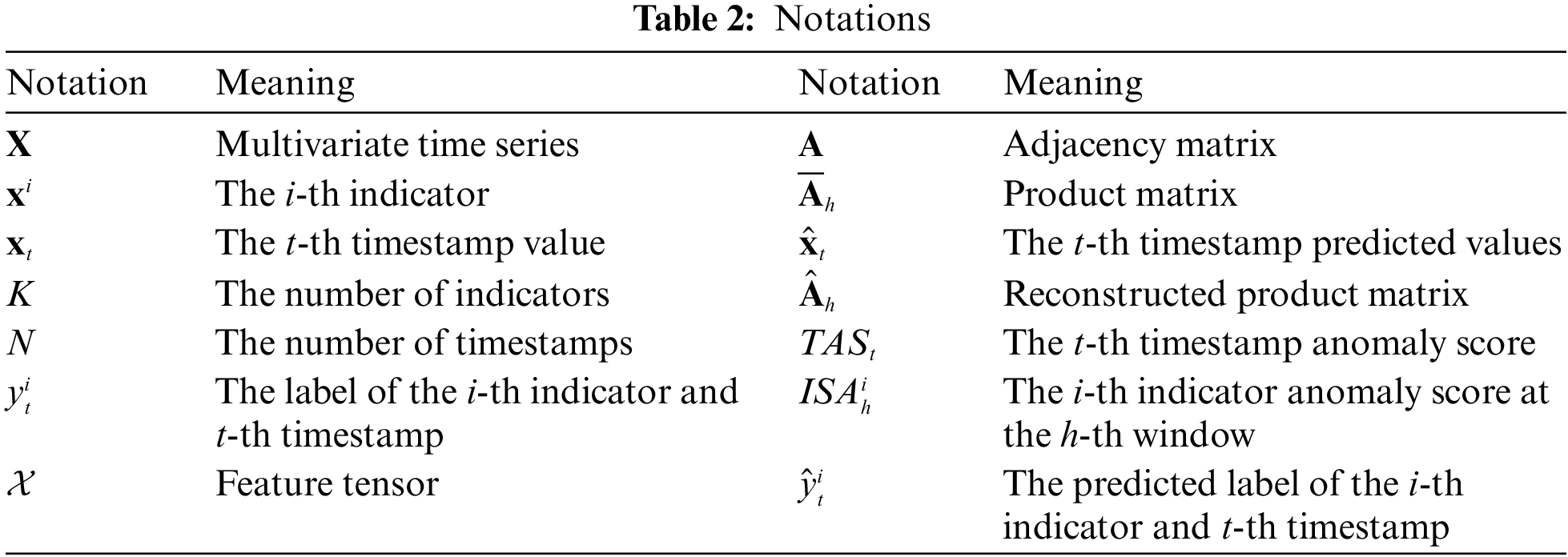
The notations in this paper are shown in Table 2. In the following sub-section, each part is described in more detail.

4.2 Data Preprocessing

This paper aims to construct a graph structure representing the relationship between the indicators. The graph contains K nodes, each of which represents an indicator and has its feature. The edges represent the relationship between indicators, while the data for the prediction and reconstruction models are independently processed.

4.2.1 Preprocessing for Prediction Model

The multivariate time series is divided into a set of multivariate sub-sequences by a sliding window with window size wp and step size 1. The t-th multivariate sub-sequence, denoted as Xt=(xt−wp,xt−wp+1,…,xt−1)∈RK×wp, is used to predict the value at timestamp t, where t={wp+1,wp+2,…,N}. There are a total of H multivariate sub-sequences, where H=N−wp+1. All multivariate sub-sequences constitute a feature tensor 𝒳∈RH×K×wp.

Based on the multivariate time series X, the cosine similarity is exploited to measure the similarity between indicators. An adjacency matrix A∈RK×K is constructed based on the top S similarity. The top S similarity is set to 1 to indicate that the two nodes are adjacent, while the remaining values are set to 0 in the adjacency matrix, which can be formulated as follows:

eij=xiTxj‖xi‖×‖xj‖,i,j∈{1,2,…,K}(1)

Aij=1{eij∈Top S}(2)

where Aij represents the adjacency relationship between the i-th and j-th indicators.

4.2.2 Preprocessing for Reconstruction Model

The multivariate time series is divided into a set of multivariate sub-sequences by a fixed window with window size wr. The h-th multivariate sub-sequence is denoted by X¯h=(xh×wr,…,x(h+1)×wr−1)∈RK×wr, where h={0,1,…,H¯−1} and H¯=N/wr. There are a total of H¯ multivariate sub-sequences. The related H¯ product matrices form the product tensor 𝒜¯∈RH¯×K×K.

For the multivariate sub-sequence, this paper uses the inner product between indicator pairs to represent the adjacency relationship between indicator pairs in a given window, which can be represented by a product matrix A¯h∈RK×K. The element of the i row and j column in the h-th product matrix is formulated as follows:

A¯hij=(xh×wri,…,x(h+1)×wr−1i)×(xh×wrj,…,x(h+1)×wr−1j)T(3)

where (xh×wri,…,x(h+1)×wr−1i)T represents the sub-sequence of the i-th indicator on the h-th multivariate sub-sequence.

4.3 GAT-based Prediction Model

To predict the following values and detect abnormal timestamps, this paper adopts a feature extractor based on GAT. GAT fuses the feature of an individual node with those of its neighbors according to the graph structure learned from data preprocessing. In more detail, this paper obtains the aggregated representation zti of node i at t timestamp as follows:

zti=ReLU(αiiWXti+∑j∈N(i)αijWXtj)(4)

Xti=(xt−wpi,xt−wp+1i,…,xt−1i)(5)

where xt−wpi is the value of node i at timestamp t−wp, N(i)={j,Aij>0} is the neighbor node set of node i, W∈Rd×wp is the weight matrix needing to be trained, d is the dimension of hidden features, and αij is the attention coefficient, which can be calculated as follows:

π(i,j)=LeakyRelu(aT(WXti⊕WXtj))(6)

αij=exp⁡(π(i,j))∑k∈N(i)∪{i}exp⁡(π(i,k))(7)

Here, ⊕ represents concatenation, while α is the learnable coefficient vector of the attention mechanism. This paper uses LeakyReLU as a non-linear activation to calculate the attention coefficient and softmax function to normalize the attention coefficient in Eq. (7).

This paper extracts the aggregated representations of all nodes at timestamp t by a stacked fully connected layer with dimension K to predict the value at timestamp t, denoted by x^t:

x^t=fθ([zt1,…,ztK])(8)

where zti is the aggregate value of node i at timestamp t. The mean square error between the predicted output x^t and the ground truth xt are taken as the loss function:

LMSE=1N−wp∑t=wp+1N||x^t−xt||2(9)

Based on these learned relationships, this paper can detect and explain anomalies that deviate from these relationships. The predicted value and the ground truth value are compared to obtain an error value Errti at node i and timestamp t:

Errti=|xti−x^ti|(10)

where xti,x^ti are the ground truth and prediction of node i at timestamp t and |⋅| is the absolute value function. Subsequently, a max function is exploited to obtain an overall time anomaly score (TAS) at timestamp t by aggregating the error of all nodes:

TASt=maxiErrti(11)

Finally, when TASt exceeds a fixed threshold θ, timestamp t is identified as anomalous. Different methods can be used to set the threshold, such as extreme value theory [30]. This paper uses the maximum value as the threshold in the validation dataset.

4.4 A-ConvLSTM-based Reconstruction Model

This component extracts the relationship among indicators via convolutional neural networks and the temporal feature of the relationship via attention-based convolutional LSTM networks(A-ConvLSTM) to capture the dynamic relationship among indicators.

This model uses a convolutional encoder to encode the inter-correlation between indicators and an A-ConvLSTM to capture the temporal patterns of the inter-correlations, as shown in Fig. 5. Subsequently, a convolutional decoder is used to reconstruct the input based on the feature mapping of the inter-correlation and temporal patterns. After the decoder, the reconstructed error is used to detect and diagnose abnormal indicators.

Figure 5: The framework of the reconstruction model. It consists of three parts: convolutional encoder, A-ConvLSTM network, and convolutional decoder

The product tensor 𝒜¯∈RH¯×K×K is the input. The next m product matrices in the product tensor 𝒜¯ are fed into this model, which can be denoted by 𝒢h0=[A¯h−m+1,…,A¯h−1,A¯h]∈Rm×K×K. This model aggregates the information in these m product matrices and reconstructs the product matrices themselves.

4.4.1 Convolutional Encoder

To capture the inter-correlations among indicators, four-layer convolution neural networks are performed on the input product tensor 𝒢. The convolution operation is specifically expressed as follows:

𝒢hl=σ(Wl∗𝒢hl−1+bl)(12)

where * is the convolution operation, σ is the activation function, 𝒢hl is the spatial feature tensors of the h-th product tensor after the l-th convolution, and Wl,bl denote the convolutional kernel and bias in the l-th layer.

4.4.2 A-ConvLSTM

The spatial feature tensors in the convolutional encoder are temporally dependent on previous time steps. A-ConvLSTM is used to capture the temporal information in the spatial feature tensors sequence inspired by ConvLSTM. Reference [31] shows further details of ConvLSTM.

Given the spatial feature tensor 𝒢hl from the l-th convolutional layer and the previous hidden state ℋh−1l∈Rml×Kl×Kl, the current hidden state ℋhl is updated by ℋhl=ConvLSTM(𝒢hl,ℋh−1l).

Not all previous steps are equally correlated to the current state. This paper combines ℋhl with the previous hidden states by the attention mechanism to form a refined hidden representation ℋ¯hl∈Rml×Kl×Kl. Because of four convolutional layers, it generates four refined hidden representations ℋ¯h1,ℋ¯h2,ℋ¯h3,ℋ¯h4:

ℋ¯hl=∑v∈(h−m+1,h)αvℋvl(13)

αv=exp⁡{σ(aT(ℋhl⊕ℋvl))}∑v∈(h−m+1,h)exp⁡{σ(aT(ℋhl⊕ℋvl))}(14)

where α is the attention coefficient, σ is the activation function, and a is the learnable coefficient vector of the attention mechanism.

4.4.3 Convolutional Decoder

To decode the feature tensors and reconstruct the product matrices, the convolutional decoder works in reverse order. This paper first convolves the refined hidden representation ℋ¯h4 of the fourth layer to obtain ℋ^h3. Then, in the third, second, and first layers, the ℋ^hl is concatenated with the refined hidden representation ℋ¯hl of the previous layer to generate matrix representation ℋ^hl−1. The ℋ^h0 is the reconstructed product matrix:

ℋ^hl−1={σ(W^l⊗ℋ¯hl+b^l),l=4σ(W^l⊗[ℋ^hl⊕ℋ¯hl]+b^l),l=3,2,1}(15)

A^h=Last(ℋ^h0)(16)

where ⊗ is the deconvolution operation, ⊕ is the connection operation, W^l,b^l are the deconvolutional kernel and bias in the l-th layer, σ is the activation function (same as the encoder), Last(⋅) refers to taking the last matrix of the tensor, and A^h∈RK×K is the reconstructed product matrix of the h-th product matrix A¯h. The loss function is the root mean square error between the reconstructed product matrix and the raw product matrix.

LRMSE(A^h,A¯h)=1K2∑i=1K∑j=1K(A^hij−A¯hij)2(17)

4.4.4 Anomaly Score

The error matrix is made up of the differences between the reconstructed product matrix A^h and the raw product matrix A¯h, denoted by Eh∈RK×K, where:

Eh=|A^h−A¯h|(18)

There are two metrics used to identify abnormal indicators: an anomaly threshold λ and an anomaly probability threshold γ. If an element in the error matrix is greater than the anomaly threshold, it is deemed abnormal. The indicator anomaly score (ISA) is defined as the ratio of the number of abnormal elements in a row and a window.

IAShi=Count[Ehi>λ]/wr(19)

Here, IAShi is the indicator anomaly score of the i-th indicator in the h-th product matrix, Count() represents the sum of the quantities that meet the requirements, and Ehi is the i-th row of the h-th error matrix. When it exceeds the anomaly probability threshold γ, the i-th indicator at the h-th time window is deemed abnormal.

4.5 Anomaly Diagnosis

The GAT-based prediction model detects the abnormal timestamp xt and the A-ConvLSTM-based model detects the abnormal sub-indicator X¯hi=(xh×wri,…,x(h+1)×wr−1i). Combining the abnormal timestamp and the abnormal sub-indicator is fine-grained anomaly detection. This paper next needs to determine whether the abnormal timestamp is within the time window located by the abnormal sub-indicator. If the timestamp t belongs to window h (t∈{h×wr,…,(h+1)×wr−1}), there is an intersection between the timestamp and sub-indicator. This intersection is a fine-grained anomaly, which means that indicator i is abnormal at timestamp t (y^ti=1). The anomaly diagnosis algorithm is presented in Algorithm 1.

5  Performance Analysis

5.1 Datasets

The Safe Water Treatment (SWaT) dataset2 is derived from the water treatment testbed coordinated by the Public Utilities Authority of Singapore. It is a realistic Industrial Internet of Things system that requires protection from malicious attacks. SWaT contains examples of real-life attack scenarios. In total, 23 attacks are launched in SWaT. Table 3 presents the statistics of SWaT. Due to the huge amount of raw data, downsampling is performed by taking the median value of the raw data every 10 s. Once there is an anomaly in the 10 seconds, it is labeled as abnormal. There are 46 indicators in SWaT. The test dataset contains 44990 timestamps and 2069540 (=46×44990) fine-grained points. There are 4541 abnormal timestamps, and the anomaly rate is 10.1%. Moreover, the number of fine-grained anomalies is 9850, and the anomaly rate is only 0.476%.

5.2 Baselines

This paper considers five timestamp anomaly detection methods as the baseline.

•   Univariate fully connected autoencoder (UAE): It trains a separate Autoencoder (AE) for each indicator.

•   Temporal convolutional network AE (TCN AE): It exploits the TCN model [32] as the encoder and decoder of AE.

•   OmniAnomaly [6]: It uses a Gated Recurrent Unit (GRU) to capture complex temporal correlations between multivariate time series.

•   MSCRED [13]: It detects the anomaly, identifies the root cause, and interprets anomaly severity by an attention-based convolutional LSTM.

•   GDN [11]: It uses an attention-based graph neural network to learn the dependence relationships between time series and predict future behavior.

Two extension methods are applied to all five baseline methods for the FGAD task.

•   ATop: It directly takes the top M anomaly score of all indicators on all timestamps as anomalies.

•   PTop: It takes the top M anomaly score of all indicators on the abnormal timestamps identified by the timestamp anomaly detection method as anomalies.

5.3 Parameters Settings and Evaluation Metrics

In terms of the parameters in the GAT-based prediction model, the Adam optimizer is used for training, the learning rate is 1×10−3, the window size wp is 30, and the number of neighbors S is set to 15. In terms of the parameters in the A-ConvLSTM-based reconstruction model, the Adam optimizer is used for training with a learning rate of 1×10−4. The window size wr is 5. The number of input product matrices m is set to 5. For ATop and PTop extension methods, the top M is set to 9000 according to the percent of anomalies in the FGAD task. The parameters of the fully convolutional layer in the encoder are as follows: 32 kernels of size 3×3×3, 64 kernels of size 3×3×32, 128 kernels of size 2×2×64, and 256 kernels of size 2×2×128, along with strides of 1×1, 2×2, 2×2, and 2×2. The parameters of the deconvolution layer in the decoder are as follows: 128 kernels of size 2×2×256, 64 kernels of size 2×2×128, 32 kernels of size 3×3×64, and three kernels of size 3×3×64 filters, along with strides of 2×2,2×2,2×2, and 1×1. The parameter settings are listed in Table 4. All experiments are run on a server with an Intel i7-9700 CPU, RTX 2080 SUPER GPU, and 32 GB RAM, as well as with Python 3.7 and Pytorch 1.1.8.

This paper uses precision (Prec), recall (Rec), F1 score (F1), Receiver Operating Characteristic (RoC), Area under Curve (AUC), HitRate@100 (HR@100), and HitRate@150 (HR@150) to evaluate the performance of our method. The HitRate@100 and HitRate@150 metrics give the average fraction of overlap between the true anomalous indicators and the top 1.0x and 1.5x indicators on the anomalous timestamps. Precision, recall, and F1 score based on ATop or PTop rewards identify the anomalous indicators from several timestamps, while hit rate metrics reward identifying the anomalous indicators from each timestamp. This paper considers two cases according to the availability of the ground truth of anomalous timestamps for hit rate metrics:

•   Tp-det: The ground truth of anomalous timestamps is unknown. Only the detected anomalous timestamps are considered. Different methods detect different anomalous timestamps.

•   Tp-all: The ground truth of anomalous timestamps is known, and all abnormal timestamps are considered. All detection methods have the same abnormal timestamps.

5.4 Experimental Results

The anomaly detection results in terms of precision, recall, and F1 score on SWaT are shown in Table 5. All five methods with PTop outperform ATop. The reason is that PTop is based on the abnormal timestamp and then in-depth look up the fine-grained anomalies of the abnormal indicator. In this way, the scope of anomaly identification is reduced. In the following experiment, only the PTop extension is considered for comparison with MFGAD. The proposed algorithm MFGAD significantly outperforms all five methods because it considers the dynamic relationship between indicators. The ROC and AUC of the six methods are shown in Fig. 6. MFGAD achieves the highest AUC (0.92) with the benefit of two independent sub-models for timestamp and indicator detection.

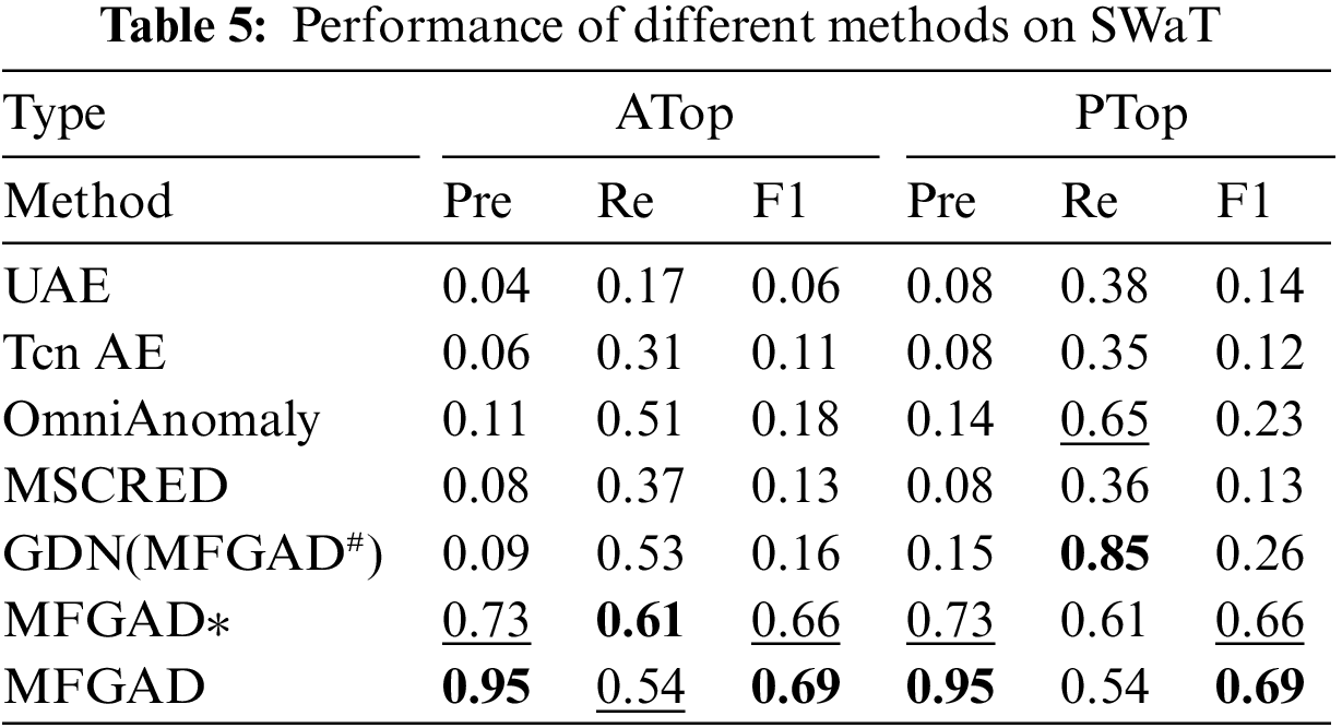
Figure 6: The ROC and AUC of different methods

The effect of the two sub-models is also considered. The TSAD sub-model is denoted by MFGAD# , which is the same as GDN, and the IAD sub-model is denoted by MFGAD*. The TSAD sub-model only provides anomalous timestamps and needs to be extended. Therefore, the F1 score of the TSAD sub-model is low. The IAD sub-model provides anomalous indicators with a window, which can achieve a reasonable F1 score. MFGAD achieves a 4% more F1 score compared with the IAD sub-model. The reason is that the TSAD sub-model filters the normal timestamps from the abnormal window.

Table 6 shows the hit rate results for six methods. Four methods, except OmniAnomaly and MFGAD, have lower hit rate metrics at the detected anomalous timestamps (Tp-det) than at all anomalous timestamps (Tp-all). That means that an algorithm that is good at ranking the indicator-wise score correctly at all anomalous timestamps, may not be good at ranking the indicator-wise scores correctly at their detected timestamps. However, the detected anomalous timestamps also depend on aggregating the indicator-wise scores. A good indicator-wise score ranking may not lead to a good aggregation score ranking because of the different aims between TSAD and FGAD. MFGAD can detect more anomalous indicators in both the detected and all anomalous timestamps.

5.5 The Impact of Window Sizes

The window size setting affects the anomaly detection performance. In the following experiment, this paper considers the influence of window size on the GAT-based prediction model and theA-ConvLSTM-based reconstruction model.

The window size wp is set to 10, 30, 50, 80, and 100, while other parameters are set to their default values to investigate the effect of window size on the GAT-based prediction model. The anomaly detection results are shown in Fig. 7. The window size of the prediction model is found to have little effect on MFGAD. When the window size is 30, the F1 scores of the two methods reach their highest values. When the window size is largest, the performance of MFGAD decreases slightly. However, when the window size is 10 or larger than 30, the performance of PTop-GDN reduces significantly.

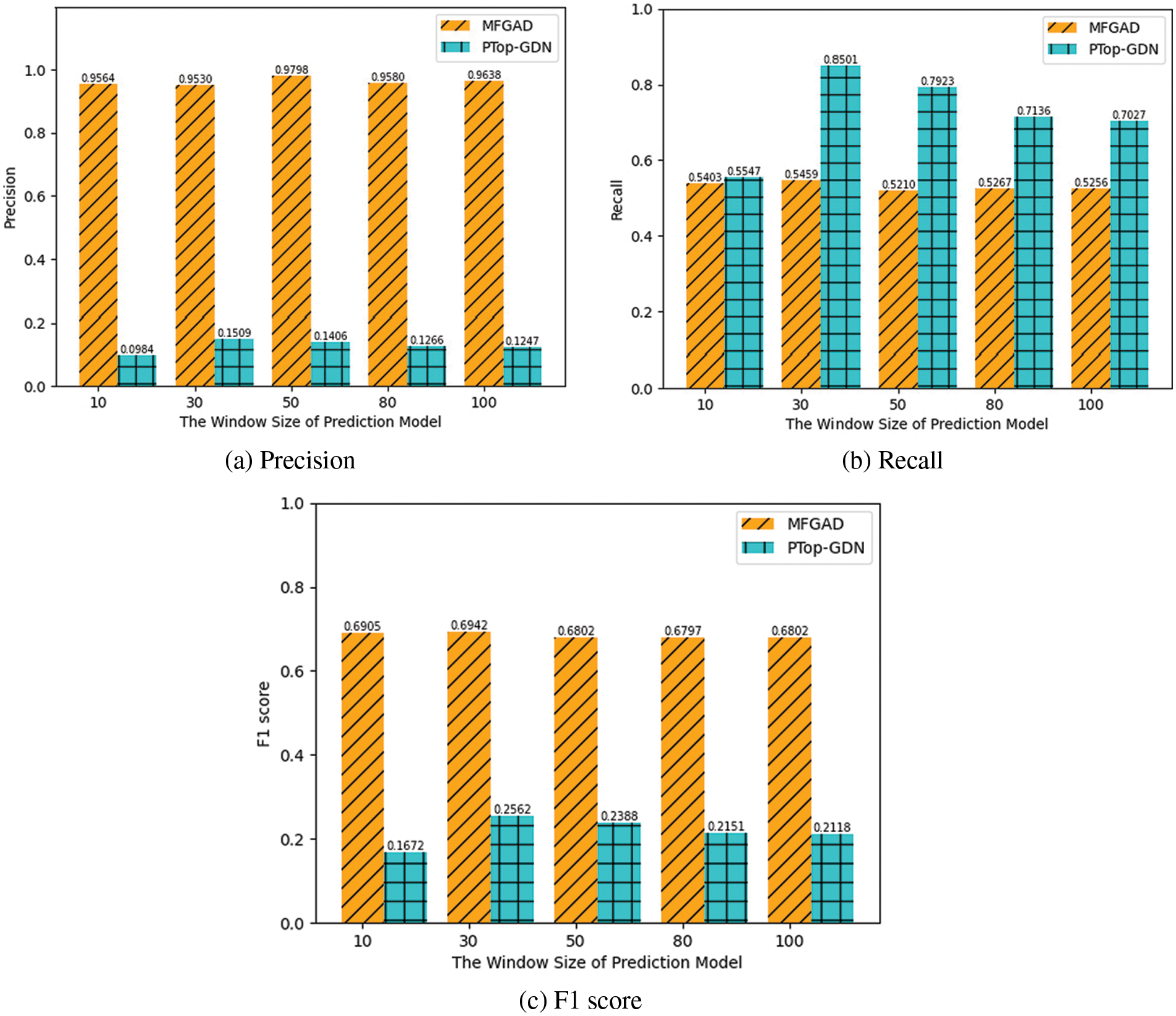
Figure 7: The experimental results with different window sizes for the GAT-based prediction model

The window size wr is set to 5, 10, 30, 50, and 80, while other parameters are set to their default values to investigate the effect of window size on the A-ConvLSTM-based reconstruction model. The anomaly detection results are shown in Fig. 8. There is no reconstruction model in PTop-GDN, and its performance remains stable. The window size of the reconstruction model is found to have a significant impact on MFGAD. Precisely, the larger the window size, the more difficult it is for the reconstruction model to detect abnormal indicators with a short duration, which reduces the performance of MFGAD. When the window size is 5, the F1 score of MFGAD is optimal. The proposed MGFAD is thus significantly better than the latest extended methods.

Figure 8: The experimental results with different window sizes for the A-ConvLSTM-based reconstruction model

6  Conclusion and Future Work

This paper proposes the MFGAD framework to tackle the FGAD problem, which consists of two sub-models to independently identify the abnormal timestamp and abnormal indicator instead of a single model. Based on the framework, this paper implements a GAT-based prediction model and anA-ConvLSTM-based reconstruction model that extracts the feature in the timestamp and indicator dimension, then combines them to identify fine-grained anomalies. Simulation experiments on a real-world dataset show that the proposed MFGAD can achieve a better F1 score and hit rate compared with the latest extended methods. However, the two sub-model of MFGAD lead to a high computational cost. In future work, the prediction model and reconstruction model in the framework can be further reduced their computational cost.

Acknowledgement: The authors would like to thank the anonymous reviewers for their valuable comments and suggestions that improve the presentation of this paper.

Funding Statement: This work was supported in part by the National Natural Science Foundation of China under Grant 62272062, the Researchers Supporting Project number. (RSP2023R102) King Saud University, Riyadh, Saudi Arabia, the Open Research Fund of the Hunan Provincial Key Laboratory of Network Investigational Technology under Grant 2018WLZC003, the National Science Foundation of Hunan Province under Grant 2020JJ2029, the Hunan Provincial Key Research and Development Program under Grant 2022GK2019, the Science Fund for Creative Research Groups of Hunan Province under Grant 2020JJ1006, the Scientific Research Fund of Hunan Provincial Transportation Department under Grant 202143, and the Open Fund of Key Laboratory of Safety Control of Bridge Engineering, Ministry of Education (Changsha University of Science Technology) under Grant 21KB07.

Conflicts of Interest: The authors declare that they have no conflicts of interest to report regarding the present study.

1Here, “indicator” refers to the time series of a particular variable.

2https://itrust.sutd.edu.sg/testbeds/secure-water-treatment-swat

References

1. B. Xiong, K. Yang, J. Zhao and K. Li, “Robust dynamic network traffic partitioning against malicious attacks,” Journal of Network and Computer Applications, vol. 87, no. 7, pp. 20–31, 2017. [Google Scholar]

2. Z. Xia, G. Long and B. Yin, “Confidence-aware collaborative detection mechanism for false data attacks in smart grids,” Soft Computing, vol. 25, no. 7, pp. 5607–5618, 2021. [Google Scholar]

3. K. Hundman, V. Constantinou, C. Laporte, I. Colwell and T. Soderstrom, “Detecting spacecraft anomalies using lstms and nonparametric dynamic thresholding,” in Proc. of the 24th ACM SIGKDD Int. Conf. on Knowledge Discovery & Data Mining, London, UK, pp. 387–395, 2018. [Google Scholar]

4. D. Park, Y. Hoshi and C. C. Kemp, “A multimodal anomaly detector for robot-assisted feeding using an lstm-based variational autoencoder,” IEEE Robotics and Automation Letters, vol. 3, no. 3, pp. 1544–1551, 2018. [Google Scholar]

5. B. Zong, Q. Song, M. R. Min, W. Cheng, C. Lumezanu et al., “Deep autoencoding Gaussian mixture model for unsupervised anomaly detection,” in 6th Int. Conf. on Learning Representations, ICLR 2018, Vancouver, BC, Canada, pp. 1–19, 2018. [Google Scholar]

6. Y. Su, Y. Zhao, C. Niu, R. Liu, W. Sun et al., “Robust anomaly detection for multivariate time series through stochastic recurrent neural network,” in Proc. of the 25th ACM SIGKDD Int. Conf. on Knowledge Discovery & Data Mining, Anchorage, AK, USA, pp. 2828–2837, 2019. [Google Scholar]

7. D. Li, D. Chen, B. Jin, L. Shi, J. Goh et al., “Mad-gan: Multivariate anomaly detection for time series data with generative adversarial networks,” in Int. Conf. on Artificial Neural Networks, Munich, Germany, pp. 703–716, 2019. [Google Scholar]

8. Q. He, Y. J. Zheng, C. Zhang and H. Wang, “MTAD-TF: Multivariate time series anomaly detection using the combination of temporal pattern and feature pattern,” Complexity, vol. 2020, no. 1, pp. 8846608–8846609, 2020. [Google Scholar]

9. H. Zhao, Y. Wang, J. Duan, C. Huang, D. Cao et al., “Multivariate time-series anomaly detection via graph attention network,” in 20th IEEE Int. Conf. on Data Mining, Sorrento, Italy, pp. 841–850, 2020. [Google Scholar]

10. J. Audibert, P. Michiardi, F. Guyard, S. Marti and M. A. Zuluaga, “Usad: Unsupervised anomaly detection on multivariate time series,” in Proc. of the 26th ACM SIGKDD Int. Conf. on Knowledge Discovery & Data Mining, Virtual Event, CA, USA, pp. 3395–3404, 2020. [Google Scholar]

11. A. Deng and B. Hooi, “Graph neural network-based anomaly detection in multivariate time series,” in Proc. of the AAAI Conf. on Artificial Intelligence, Virtual Event, pp. 4027–4035, 2021. [Google Scholar]

12. A. Garg, W. Zhang, J. Samaran, R. Savitha and C. -S. Foo, “An evaluation of anomaly detection and diagnosis in multivariate time series,” IEEE Transactions on Neural Networks and Learning Systems, vol. 33, no. 6, pp. 2508–2517, 2021. [Google Scholar]

13. C. Zhang, D. Song, Y. Chen, X. Feng, C. Lumezanu et al., “A deep neural network for unsupervised anomaly detection and diagnosis in multivariate time series data,” in Proc. of the AAAI Conf. on Artificial Intelligence, Honolulu, Hawaii, USA, pp. 1409–1416, 2019. [Google Scholar]

14. D. Cao, K. Zeng, J. Wang, P. K. Sharma, X. Ma et al., “Bert-based deep spatial-temporal network for taxi demand prediction,” IEEE Transactions on Intelligent Transportation Systems, vol. 23, no. 7, pp. 9442–9454, 2022. [Google Scholar]

15. J. Wang, Y. Tang, S. He, C. Zhao, P. K. Sharma et al., “Logevent2vec: Logevent-to-vector based anomaly detection for large-scale logs in internet of things,” Sensors, vol. 20, no. 9, pp. 2451, 2020. [Google Scholar] [PubMed]

16. N. Liao and X. Li, “Traffic anomaly detection model using k-means and active learning method,” International Journal of Fuzzy Systems, vol. 24, no. 5, pp. 2264–2282, 2022. [Google Scholar]

17. N. Liao, Y. Song, S. Su, X. Huang and H. Ma, “Detection of probe flow anomalies using information entropy and random forest method,” Journal of Intelligent & Fuzzy Systems, vol. 39, no. 1, pp. 433–447, 2020. [Google Scholar]

18. J. Zhang, W. Wang, C. Lu, J. Wang and A. K. Sangaiah, “Lightweight deep network for traffic sign classification,” Annals of Telecommunications, vol. 75, no. 7–8, pp. 369–379, 2020. [Google Scholar]

19. S. Ul Amin, M. Ullah, M. Sajjad, F. A. Cheikh, M. Hijji et al., “Eadn: An efficient deep learning model for anomaly detection in videos,” Mathematics, vol. 10, no. 9, pp. 1555, 2022. [Google Scholar]

20. X. Chen, L. Deng, F. Huang, C. Zhang, Z. Zhang et al., “Daemon: Unsupervised anomaly detection and interpretation for multivariate time series,” in 2021 IEEE 37th Int. Conf. on Data Engineering (ICDE), Chania, Greece, pp. 2225–2230, 2021. [Google Scholar]

21. Z. Li, Y. Zhao, J. Han, Y. Su, R. Jiao et al., “Multivariate time series anomaly detection and interpretation using hierarchical inter-metric and temporal embedding,” in Proc. of the 27th ACM SIGKDD Conf. on Knowledge Discovery & Data Mining, Singapore, Virtual Event, pp. 3220–3230, 2021. [Google Scholar]

22. L. Dai, T. Lin, C. Liu, B. Jiang, Y. Liu et al., “Sdfvae: Static and dynamic factorized vae for anomaly detection of multivariate cdn kpis,” in Proc. of the Web Conf. 2021, Ljubljana, Slovenia, pp. 3076–3086, 2021. [Google Scholar]

23. Z. Chen, D. Chen, X. Zhang, Z. Yuan and X. Cheng, “Learning graph structures with transformer for multivariate time series anomaly detection in IoT,” IEEE Internet of Things Journal, vol. 9, no. 12, pp. 9179–9189, 2022. [Google Scholar]

24. W. Zhang, C. Zhang and F. Tsung, “Grelen: Multivariate time series anomaly detection from the perspective of graph relational learning,” in Proc. of the Thirty-First Int. Joint Conf. on Artificial Intelligence, IJCAI-22, Vienna, Austria, pp. 2390–2397, 2022. [Google Scholar]

25. S. He, Z. Li, J. Wang and N. Xiong, “Intelligent detection for key performance indicators in industrial-based cyber-physical systems,” IEEE Transactions on Industrial Informatics, vol. 17, no. 8, pp. 5799–5809, 2021. [Google Scholar]

26. K. Xie, X. Li, X. Wang, G. Xie, J. Wen et al., “Fast tensor factorization for accurate internet anomaly detection,” IEEE/ACM Transactions on Networking, vol. 25, no. 6, pp. 3794–3807, 2017. [Google Scholar]

27. G. Xie, K. Xie, J. Huang, X. Wang, Y. Chen et al., “Fast low-rank matrix approximation with locality sensitive hashing for quick anomaly detection,” in IEEE INFOCOM 2017-IEEE Conf. on Computer Communications, Atlanta, GA, USA, pp. 1–9, 2017. [Google Scholar]

28. K. Xie, X. Li, X. Wang, G. Xie, J. Wen et al., “Graph based tensor recovery for accurate internet anomaly detection,” in IEEE INFOCOM 2018-IEEE Conf. on Computer Communications, Honolulu, HI, USA, pp. 1502–1510, 2018. [Google Scholar]

29. K. Xie, X. Li, X. Wang, J. Cao, G. Xie et al., “On-line anomaly detection with high accuracy,” IEEE/ACM Transactions on Networking, vol. 26, no. 3, pp. 1222–1235, 2018. [Google Scholar]

30. A. Siffer, P. -A. Fouque, A. Termier and C. Largouet, “Anomaly detection in streams with extreme value theory,” in Proc. of the 23rd ACM SIGKDD Int. Conf. on Knowledge Discovery and Data Mining, Halifax, NS, Canada, pp. 1067–1075, 2017. [Google Scholar]

31. S. Xingjian, Z. Chen, H. Wang, D. -Y. Yeung, W. -K. Wong et al., Convolutional lstm network: A machine learning approach for precipitation nowcasting. In: Advances in Neural Information Processing Systems. Montreal, Quebec, Canada, pp. 802–810, 2015. [Google Scholar]

32. S. Bai, J. Z. Kolter and V. Koltun, “An empirical evaluation of generic convolutional and recurrent networks for sequence modeling,” CoRR, vol. abs/1803.01271, 2018. http://arxiv.org/abs/1803.01271 [Google Scholar]