Delivery Service Management System Using Google Maps for SMEs in Emerging Countries

1  Introduction

Southeast Asia countries are among emerging countries [1]. Most companies in emerging countries are Small and Medium Enterprises (SMEs). In the context of Industry 4.0 in Logistics and Supply Chain Management, SMEs that own delivery fleets are using Internet of Things (IoT) technologies such as a Global Positioning System (GPS) and Google Maps applications. Some SMEs use a GPS tracking system for tracking the location and status of a truck in real time. Others use Google Maps apps on smartphones for navigating directions to customers that drivers have never visited there before. The SMEs in emerging countries need a Delivery Service Management (DSM) system to support their employees to manage delivery services.

This paper develops the DSM system to be beneficial for SMEs in emerging countries with the following characteristics. First, SMEs are firms that have between 20 and 200 employees [1]. They own the delivery fleets of (no more than 10) pickup trucks and hire permanent drivers. They provide Business-to-Business (B2B) delivery services to customers. Each customer orders a relatively high volume (quantity and weight) of goods. Second, potential customers are located in wide areas where trucks have to travel through free-flow and congested traffic roads. SMEs often receive orders from new customers and have no historical delivery data for them. Third, employees who manage the delivery fleets might not be technical experts in Logistics and Supply Chain. They have limited knowledge of delivery fleet management. They dislike a large and complicated system but need a simple and flexible one. Fourth, SMEs have a limited budget to invest in technologies and commercial software to support employees in managing delivery services.

There are several existing studies related to the development of DSM systems. First, Habault et al. [2] developed a delivery management system prototype to manage electric scooters for food deliveries. This prototype system consists of five core mechanisms: a communication system, a machine-learning algorithm, a sharing algorithm, a routing algorithm, and a view system. Similar commercial applications include Foodpanda and GrabFood applications. Second, Kandakoglu et al. [3] developed a Home Dialysis Scheduler (HDS) system for home dialysis visit scheduling and nurse routing. The HDS system assists with dialysis treatments in patients’ homes. It was designed as a stand-alone, single installation system with all the required software and database locally stored. The HDS system consists of a user interface module, a visualization module, a report generation module, an optimization module, a data module, and a map module. The HDS system was implemented using Java scripts and open-source libraries. Third, Lacomme et al. [4] proposed a Mapotempo Transportation system to assist route managers in complex decision-making processes. The system was implemented through a Representational State Transfer (REST) based on Application Programming Interface (API). The optimizer API used various state-of-the-art operational methods. This system is a web application and has been used in practice by the Mapotempo company.

The existing systems in [2–4] have some limitations for application to SMEs in emerging countries. The prototype system in [2] is suitable for Business-to-Customer (B2C) delivery services within a limited road network. It is difficult to extend for managing B2B delivery services. The HDS system in [3] provides the sequence of patient visits. However, it does not provide the detail of real road segments used for nursing staff traveling from one patient’s home to the next patient’s home. The Mapotempo Transportation system in [4] is a large and complicated commercial software. It requires delivery fleet managers to be experts in delivery fleet management. Most SMEs have some limitations and requirements that do not match the standard functions of commercial software. Thus, SMEs cannot afford the investment in this system. This research aims to develop a DSM system for SMEs with the above characteristics.

This paper has objectives as follows:

1.   To develop a Delivery Service Management (DSM) system for SMEs that own a delivery fleet of pickup trucks. This system is suitable for Business-to-Business (B2B) delivery of goods where each customer orders a relatively high volume (quantity and weight) of goods.

2.   To demonstrate a real application of the developed DSM system to a Thai SME.

3.   To propose techniques to improve the accuracy of the Arrival Time Prediction (ATP) system.

4.   To prove that the proposed techniques significantly improve the accuracy of the ATP system.

The remainder of this paper is organized as follows. First, related studies are reviewed in Section 2. Then, the proposed DSM system that integrates four systems is presented in Section 3. Next, Section 4 shows the application of the proposed DSM system to a Thai SME and the discussion of experimental results. Finally, the conclusions and recommendations are provided in Section 5.

2  Literature Reviews

To develop a DSM system for SMEs in emerging countries, the authors focus on two groups of the existing literature including delivery route planning and arrival time prediction.

2.1 Delivery Route Planning

Delivery Route Planning (DRP) is also known as the Vehicle Routing Problem (VRP). This research has been popular in academic and private sectors to develop efficient DRP methods for planning the delivery routes of vehicles [5,6]. In this paper, SMEs’ delivery service is considered as the Capacitated VRP (CVRP). There are two groups of methods used for the CVRPs [7]. They are exact algorithms and approximate algorithms. Brand-and-bound algorithms and branch-and-cut-and-price algorithms are two exact algorithms that can find the optimal solutions of the CVRPs. Fukasawa et al. [8] and Marques et al. [9] developed Mixed Integer Linear Programming (MILP) models and then solved them by using IBM ILOG CPLEX Optimizer. However, the exact algorithms have a drawback. They can only solve small-sized problems and take a long computational time for large-sized problems.

In contrast, the approximate algorithms can find near-optimal solutions for large-sized problems within a reasonable time. They include classic heuristics and metaheuristics. A popular classical heuristic is the Cluster-First Route-Second (CFRS) heuristic. It divides the CVRPs into two stages: clustering and routing [10,11]. For clustering, customers are assigned to clusters, and each cluster is assigned to a different vehicle. For routing, a route is constructed for the customers in each cluster. Comert et al. [10] applied K-means algorithms and branch-and-bound algorithms for clustering and routing, respectively. Horng et al. [11] proposed LP-based CFRS heuristics to improve the quality of solutions for the CVRP with multiple objectives. The CFRS heuristic can significantly reduce problem sizes and computational times. Popular metaheuristics include genetic algorithms, ant colony optimization algorithms, particle swarm optimization algorithms, and artificial bee colony algorithms [12–15]. These algorithms are population search-based methods. They maintain a pool of good parent solutions by continually selecting parent solutions to produce promising offspring and then updating the pool. These methods are more powerful than other DRP methods. They can generate high-quality solutions within a limited time.

The exact and approximate algorithms proposed in the above literature cannot be directly applied to SMEs considered in this paper. The first reason is that SMEs cannot afford to invest in expensive commercial software. Another reason is that most SMEs do not have employees who are experts in delivery fleet management due to the scarcity of human resources [1].

This paper considers the limited capability of employees who manage the delivery fleet of trucks, the limited investment budget of SMEs, and the availability of technologies in emerging countries to develop the DRP method. It adapts the CFRS concept to plan the delivery routes of trucks. Unlike the CFRS methods in [10,11], this paper uses the experience of planners and drivers to assign customers to trucks and construct the delivery route of each truck. It deploys Google Maps applications as supporting tools to construct a realistic route for each truck.

This paper selects Google Maps over other map applications (such as TomTom Go, Waze, Here WeGo, etc.) based on the following reasons. First, Google Maps has been available for smartphones with the Android and iOS mobile operating systems [16]. Google Maps is the most popular mapping application with more than one billion people using it every month. Second, Google Maps is available in most countries around the world including emerging countries in Southeast Asia. Third, Google Maps has the following features that are useful for delivery services. The location search features (maps, satellite, and street view modes) can identify the locations of customers. The navigation and traffic features allow drivers to select a suitable route from an origin to a destination avoiding traffic congestion. The Google My Maps (GMM) interface enables users to construct a map of a delivery route and then save or share it with other users. Google Maps Platform has cloud databases (APIs) for storing the travel times and distances of road segments. They are usable in the DSM system. Fourth, the DSM system that uses Google Maps is expected to have low capital expenditure. Even though users must enable a Google account with billing for requesting data from the Google Maps APIs, Google Maps gives free $200 credit for using Google Maps APIs every month. Fifth, Google Maps has been deployed in recent studies. Kirci [17] deployed the Google Maps interface to draw real vehicle routes for cargo transportation. Santos et al. [18] used Google Maps services to develop a web-based spatial decision support system for a Vehicle Routing Problem (VRP). The authors of [19–22] extracted average travel times and distances from the Google Distance Matrix API for solving different VRP variants. The authors of [23,24] enabled the Google Maps Direction API to extract travel times with traffic conditions of road segments for real-time delivery management systems. These studies can prove that Google Maps APIs provide accurate information on real routes, travel times, and distances.

2.2 Arrival Time Prediction

This paper uses the CFRS concept and the experiences of planners and drivers to plan the delivery routes of trucks. This step does not consider the accuracy of arrival time at each customer. Therefore, this paper needs an Arrival Time Prediction (ATP) system to predict the arrival time of each truck at each customer for each delivery route.

The ATP research has been focused on by academic and public sectors to improve the performance of public transportation modes [25]. Sometimes, the concepts of estimation and prediction are vague and used equivalently by some studies. However, they have different objectives and characteristics to consider different problems. Travel time estimation models reconstruct travel times of trips completed in the past based on data collected during the trip. The most common objective is to provide the mean travel time of a given road segment and the distribution of travel time [26]. However, travel time prediction models forecast the travel time for a road segment that the trip will start in the moment (present) or the future. They use the present traffic conditions and past data for forecasting [27].

Travel time or arrival time prediction methods can be classified as naive approaches, data-based approaches, and traffic flow theory-based approaches [25]. First, naive approaches are travel time prediction methods that are simple. They are fast in terms of computational speed and easy to implement. They are divided into instantaneous, historical, and hybrid methods [28]. Chung et al. [27] and Li et al. [29] applied naive approaches for the arrival time prediction of school buses and travel time prediction on motorways, respectively. Second, data-based approaches develop relationships between dependent and independent variables. These approaches do not require expertise in traffic theory, but they need a large amount of data. Data-based approaches are divided into parametric and non-parametric models. Time series analysis [30] and regression techniques [31,32] are two popular parametric models where relationships among dependent and independent variables are predefined. In non-parametric models, relationships are not predefined. They are obtained from the data itself along with corresponding parameters. Machine learning approaches, including Artificial Neural Networks (ANNs) [33,34] and Support Vector Machines (SVMs) [35,36], are the most popular non-parametric models for travel time prediction. They can solve complex non-linear relationships. Third, traffic flow theory-based approaches predict travel times from other traffic state variables based on theoretical models. These approaches can deliver a complete traffic state overview of a network in both spatial and temporal domains with a limited amount of data [37].

As shown in Table 1, this paper proposes the ATP algorithm that considers the following characteristics. First, the ATP algorithm takes into account the whole road network including freeways and urban roads. Second, it considers both the spatiotemporal evolution and the stochastic quality of travel time. Third, the ATP algorithm measures both the accuracy and precision of arrival time prediction. Fourth, it allows planner interactions to flexibly adjust arrival time. Driver behaviors that are factors affecting arrival times [38,39] are also considered in this paper.

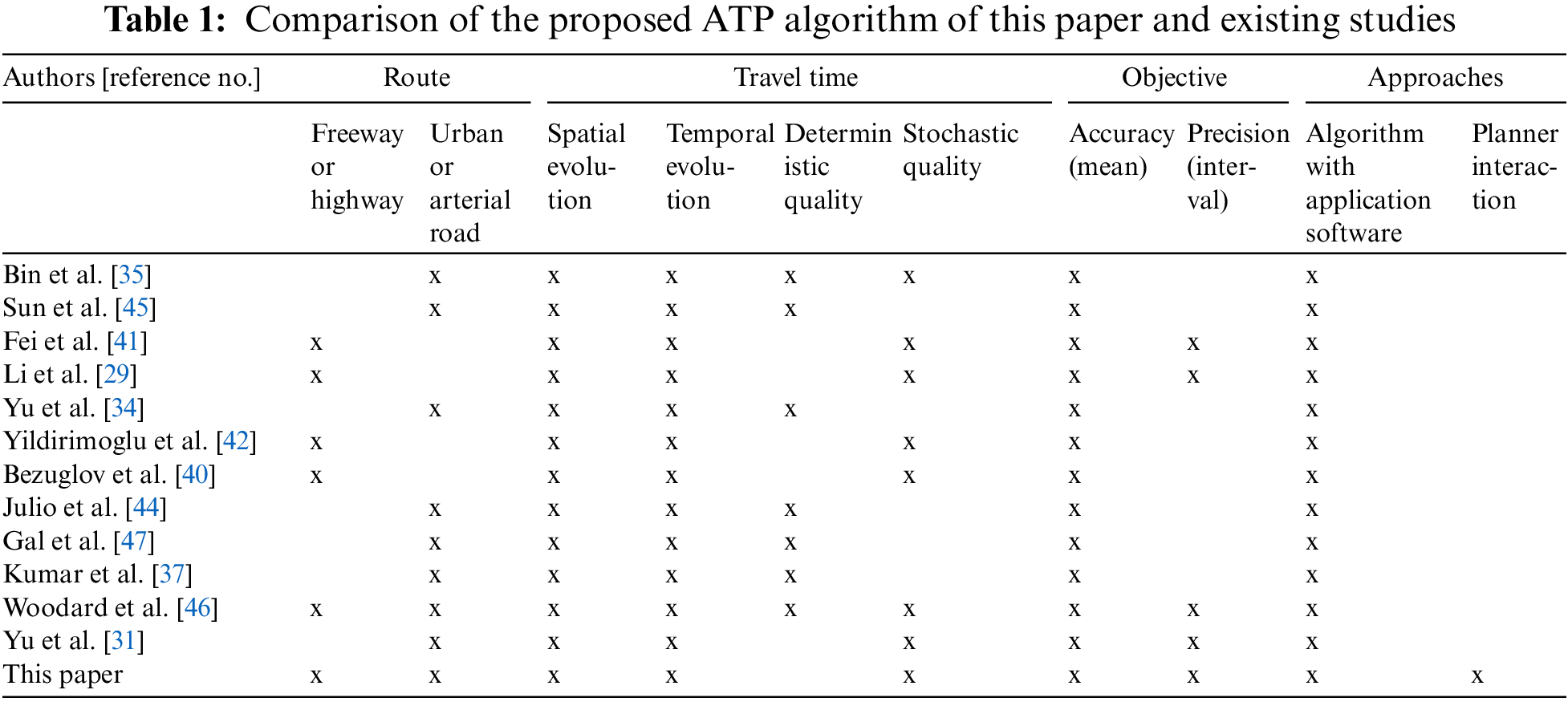
Table 1 shows the comparison between the proposed ATP algorithm and the existing prediction methods in the literature based on four main characteristics. First, most studies focused on travel time models that were restricted to short-road segments or predefined trajectories. Some studies focused on travel time models for freeway or highway segments where traffic was generally uninterrupted [40–43]. Other studies focused on bus travel time and arrival time models for urban and arterial road segments where traffic was more complex because of various factors including varying traffic congestion levels, intersection delays due to stop signs or traffic signals, and pedestrian crossing activities [44,45]. The models of these studies are usually not extended to a whole road network because the issue of missing data in certain zones leads to inadequately capturing the dynamics of the whole network. One study predicted the distribution of travel time using mobile phone GPS data considering the whole road network [46]. Second, some studies consider the evolution of travel time over space and time [45–48]. Only a few studies consider the stochastic quality of travel time [29,31,41,46]. Third, most existing prediction methods measure only the accuracy by focusing on a unique mean value of travel time or arrival time. Only a few studies measure the accuracy and precision by considering both the mean value and the confidence interval of the travel time or arrival time [29,31,41,46,49]. Fourth, from the existing prediction methods, algorithms with application software are developed, and they provide predicted values without any user interaction. An algorithm cannot address all factors of concern without user interaction decisions. If all factors are included, this results in a long computational time.

Bin et al. [35] deployed an SVM model to predict bus arrival time considering stochastic traffic conditions. The SVM model needs three input variables: segment, current segment travel time, and the latest next segment travel time. It can effectively integrate the latest bus information and accurately predict bus arrival time. Sun et al. [45] developed a bus ATP algorithm that combines GPS data with real-time estimates of interstation travel speeds. It has been implemented in an intelligent prediction system. The system can simultaneously track a large number of buses, automatically detect their service routes and directions, and predict their arrival times to downstream stations with acceptable accuracy. Yu et al. [31] proposed accelerated failure time survival models to predict the distribution of bus travel times to a downstream stop as a function of real-time operational and weather data. These models provide the expected travel times with confidence intervals. Fei et al. [41] presented a Bayesian inference-based dynamic linear model to predict online short-term travel time on a freeway stretch under stochastic traffic conditions. The proposed model provides predicted travel times with confidence intervals. It is embedded into an adaptive control system to learn and self-tune the system’s evolution noise level in response to unforeseen external events. Li et al. [29] obtained vehicle travel times from Automatic Vehicle Identification (AVI) equipment installed on a tollway. The neural network travel time prediction models were developed to predict the distribution of travel time in future periods up to 1 h ahead. Woodard et al. [46] introduced a method, called TRIP, to predict the probability distribution of travel time. TRIP uses GPS data from mobile phones or other probe vehicles. It provides accurate predictions of travel time reliability for complete, large-scale road networks.

3  Proposed Delivery Service Management System

In this section, a Delivery Service Management (DSM) system is proposed to support SMEs in emerging countries in managing delivery services. The proposed DSM system integrates four systems to manage delivery services starting from receiving the purchase orders of customers to handing over products to customers (see Fig. 1). The four systems consist of (1) a Delivery Location Positioning (DLP) system for pinpointing new delivery locations of customers; (2) a Delivery Route Planning (DRP) system for planning and visualizing the delivery route of each truck, (3) an Arrival Time Prediction (ATP) system for predicting arrival time (with an interval) at each delivery location, and (4) a Communication and Data Sharing (CDS) system for communicating and sharing information among stakeholders. The details of each system will be presented in the following sub-sections.

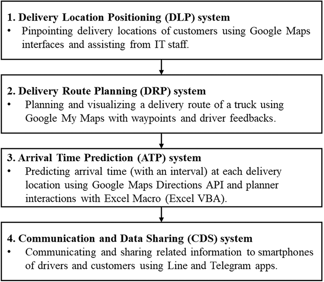
Figure 1: Overview of the Delivery Service Management (DSM) system

The DSM system uses IoT technologies, Cloud Computing, and simple mobile applications as supporting tools. The supporting tools include a GPS tracking system, Google Maps, Google Maps APIs, Google Drives, Google Sheets, an ATP algorithm embedded in Excel Macros, Line, and Telegram.

3.1 Delivery Location Positioning System

The DSM system is proposed to implement in a typical business process of SMEs as shown in Fig. 2. The DSM system requires completed and accurate information from the start of the information flow where the customer service (CS) staff receives the purchase order (PO) of a customer. The DLP system adopts the DLP method proposed by [16] for supporting SME customer services.

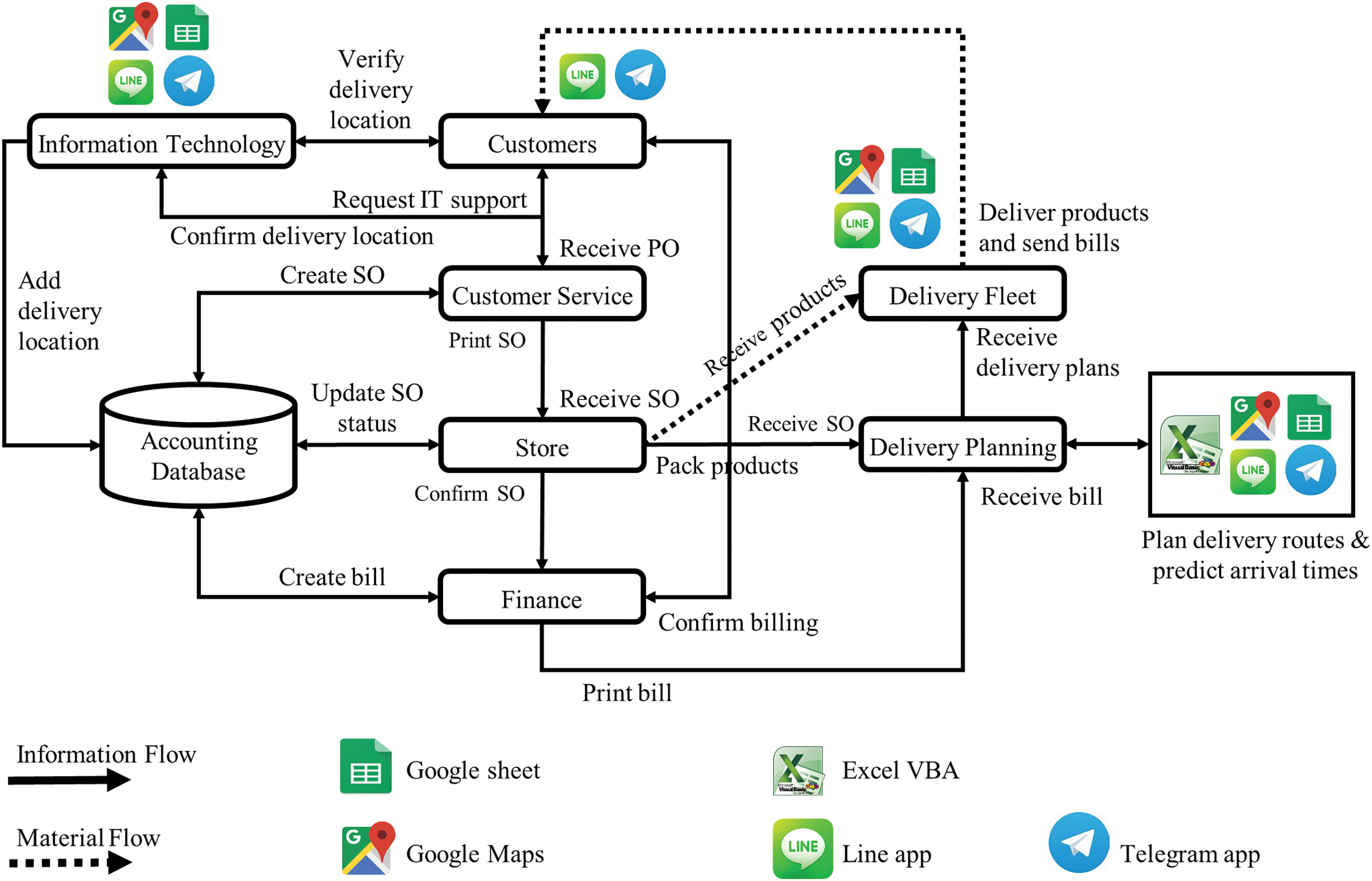
Figure 2: Implementation of the DSM system for typical SME business process

The procedure of the DLP system is described as follows. First, the CS staff needs to check the delivery location of each customer in the accounting database when receiving the PO of the customer. If the delivery location does not exist, the CS staff can request the information technology (IT) staff for assistance. Then, the IT staff communicates with the customer to obtain the accurate address and coordinates (latitude and longitude) of the delivery location by using the CDS system (see details in 3.4) and Google Maps interface. Finally, the IT staff records the address and coordinates of the delivery location in the accounting database and a Google Sheet. Thus, later they can be used by the DRP and ATP systems.

3.2 Delivery Route Planning System

For SMEs, the delivery fleet management staff (planner) is normally not an expert and has limited capability in delivery fleet management. The proposed DRP system uses Google Maps interfaces with customized features for supporting the planner to construct and visualize the delivery route of each truck. The planner uses intuitive decisions to assign customers to trucks and construct the initial delivery route of each truck. Then, the planner considers driver feedback to adjust the delivery route to be a realistic delivery route for each truck by using the waypoint technique.

The procedure of the DRP system consists of four steps as follows.

Step 1: Prepare a structured data set of customers in an Excel Workbook. The planner extracts the structured data set for customers that need delivery service on the next day of delivery from the accounting database and store it in an Excel Workbook. The structured data includes: the sales order (SO) number, name and address of each customer, ordered product list, demand quantity, address and coordinates of each delivery location, and time window (if requested).

Step 2: Assign customers to pickup trucks. The planner visualizes the depot and delivery locations of customers in a Google Maps interface, namely, Google My Maps (GMM). Then, the planner intuitively assigns the customers to trucks based on the visibility of the delivery locations in the GMM interface, the planner’s experience, and the trucks’ capacity. The planner can assign customers to trucks by using two criteria: (1) relative distances between customers, and (2) relationships between drivers and customers [11,16].

Step 3: Construct a delivery route for each pickup truck. The planner again intuitively constructs a delivery of each truck in the GMM interface and then can manually drag and drop nodes to change the sequence of customers (see Fig. 3 as an example). Note that for the route (A-B-C-D-E-F-A), A is the depot (factory), and B, C, D, E, and F are the delivery locations of customers.

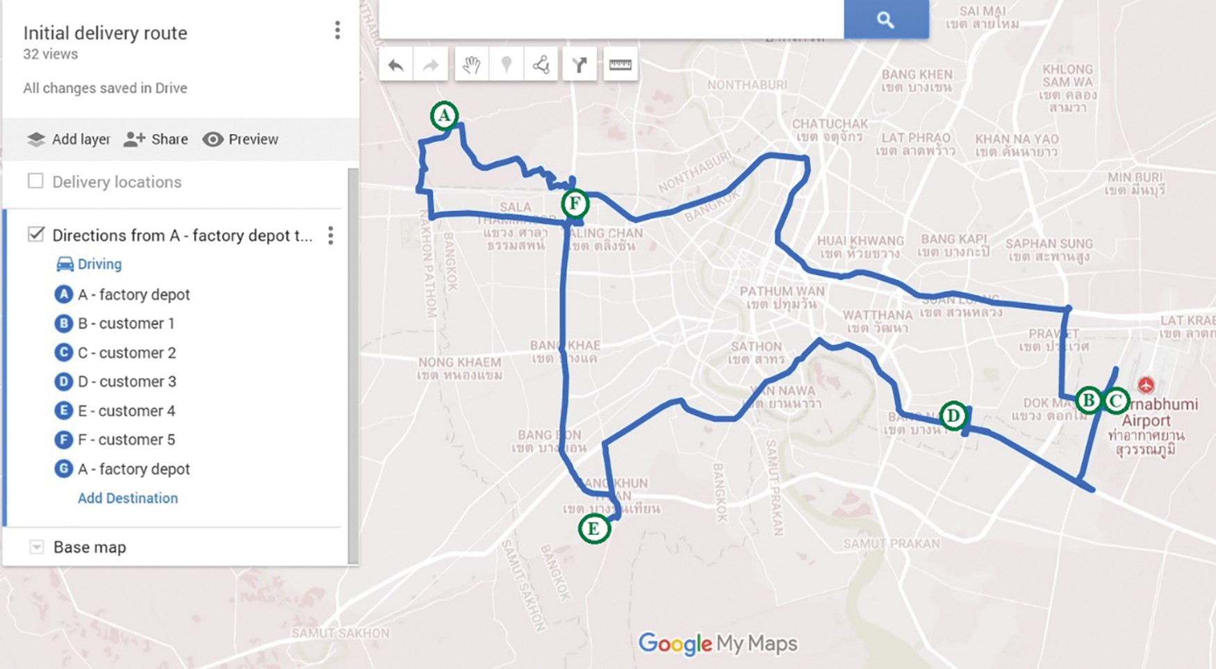
Figure 3: Initial delivery route (suggested by the GMM interface)

Step 4: Construct a realistic delivery route for each pickup truck based on driver feedback by using waypoints. The planner shares each initial route with each driver and seeks feedback. The driver can provide constructive feedback because they have knowledge and experience of the whole road network. They may know road segments that pickup trucks cannot pass such as urban roads during peak hours, a U-turn under a bridge, and a crossbar at the entrance with a height limit. The planner can insert waypoints between two nodes to adjust the delivery route based on the driver feedback. The realistic planned delivery route should follow the actual driving route avoiding restricted road segments. From Fig. 3, the GMM interface suggests route segments (A, B) and (F, A) that use urban roads. They have congested traffic and are not regular driving routes of the truck. By inserting waypoints (wp-AB1, wp-AB2, and wp-FA), these two route segments are adjusted to use detour routes as shown in Fig. 4.

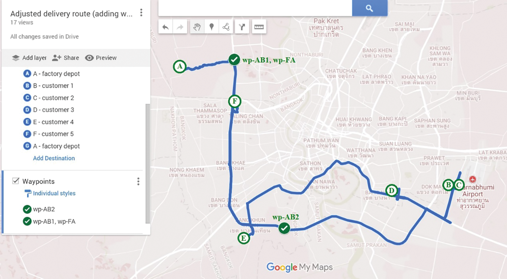
Figure 4: Adjusted delivery route by inserting waypoints

3.3 Arrival Time Prediction System

In addition to the coordinates of the depot, delivery locations, and waypoints of the delivery route obtained from the DRP system, the proposed ATP system requires the departure time of each truck from the depot and the predicted service time at each delivery location as input parameters.

The ATP system deploys an Excel Macro to extract travel times and distances from the Google Maps Directions API in real-time. It utilizes the Google travel times that are spatiotemporal-dependent and stochastic travel times (see details in 3.3.1). For the planer-driver decision, the ATP system applies three techniques for considering driver behaviors: driving a truck, serving customers, and having a lunch break. The three techniques include (1) compensation for short-distance travel time (namely, SD), allowance for a short rest after service (namely, ST), and lunch location-time estimation (namely, LT) (see details in 3.3.2).

The procedure of the ATP system is described as follows. First, the ATP system deploys the ATP algorithm embedded in an Excel Macro (see details 3.3.3) to predict arrival time (with interval) at each delivery location of customers. It uses Google travel times and the SD and ST techniques (without considering the lunch break of the driver). Second, the ATP system allows the interactions between planner-driver decisions and the ATP algorithm to consider the lunch location and duration of the driver (LT technique). Finally, the ATP system deploys the ATP algorithm again to adjust the predicted arrival time after the lunch break for the driver.

The notations of indices, sets, parameters, and variables that are formulated in this section are presented as follows:

i,j= Indices of nodes (origin and destination) of a delivery route

C=Set of customers for a delivery route, where C={1,2,…,c}

V=Set of segments for a delivery route, where V={(i,j)|i,j∈{0,C}}, and 0 is the depot

α=Significance level of 100(1−α)% confidence interval (unitless)

θ=Allowance reduction rate of travel time (min/km)

c=Number of customers for a delivery route (customers)

k=Number of factors for experimental design (factors)

m=Number of replicates for experimental design (replicates)

z=Standard normal random variable (unitless)

MAE=Mean Absolute Error of arrival time (min)

MAPE=Mean Absolute Percentage Error of arrival time (%)

RSME=Root-Mean-Square Error of arrival time (min)

dij=Google travel distance of segment (i,j) (km)

a[tij],M[tij]=Allowance and maximum allowance of travel time of segment (i,j) (min)

a[sj]=Allowance of service time at node j (min)

Ee[tij],Ep[tij]=Estimated and predicted travel time of segment (i,j) (min)

Ep[Aj],R[Aj]=Predicted and actual arrival time at node j (min)

Ee[sj],Ep[sj]=Estimated and predicted service time at node j (min)

Ee[L],Ep[L]=Estimated and predicted lunchtime of drivers (min)

Ep[Dj]=Predicted departure time at node j (min)

La,Lb=Lower and upper bound of lunchtime window [La,Lb] (min)

O[tij],P[tij]=Optimistic and pessimistic Google travel time of segment (i,j) (min)

O[Aj],P[Aj]=Earliest and latest predicted arrival time at node j (min)

Var[tij]=Variance of travel time of segment (i,j) (min2)

Var[sj]=Variance of service time at node j (min2)

Var[Aj]=Variance of arrival time at node j (min2)

Var[Dj]=Variance of departure time at node j (min2)

3.3.1 Utilization of Google Travel Times

Google travel times (GTTs) are spatiotemporal-dependent and stochastic travel times available in the Google Maps Directions API [2,16,23,24]. For each route segment, the GTTs change over the time of day for traveling. They are also available based on current traffic conditions as well as optimistic and pessimistic traffic conditions. The ATP system utilizes GTTs under the following assumptions:

•   The travel time is normally distributed.

•   The optimistic GTT is at the 5th percentile of the travel time distribution (Fig. 5a). It has a shorter duration than 95% of other travel times.

•   The pessimistic GTT is at the 95th percentile of the travel time distribution (Fig. 5b). It has a longer duration than 95% of other travel times.

•   The interval between the optimistic GTT and pessimistic GTT is the center of 90% of the travel time distribution (Fig. 5c).

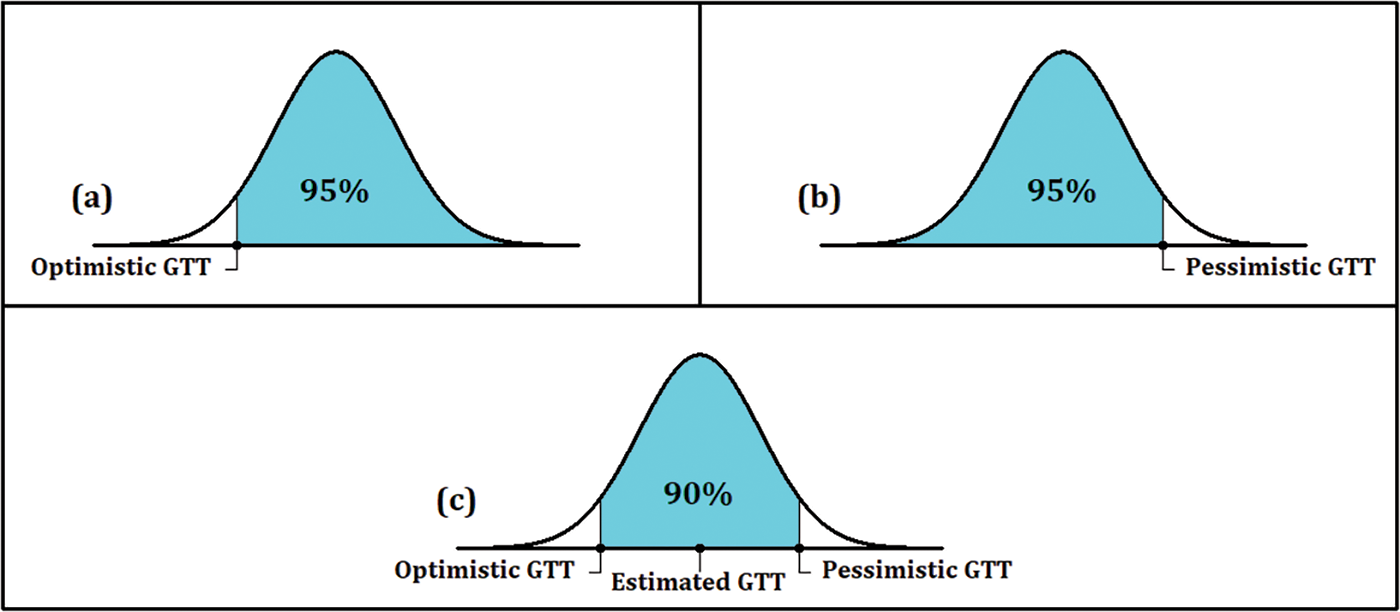
Figure 5: Normal distribution assumptions of travel time

From the above assumptions, the mean Ee[tij] and variance Var[tij] of travel time for each route segment (i,j) can be estimated from the GTTs (Montgomery & Runger, 2014, pp. 116–122) [50]. Note that i and j are the origin and destination of the route segment (i,j), respectively. First, the mean Ee[tij] of travel time is at the center of optimistic GTT O[tij] and pessimistic GTT P[tij] (see Fig. 5c and Eq. (1)). Second, the variance Var[tij] of travel time is derived as follows. If P[tij] is a normal random variable of travel time with the mean Ee[tij] and the variance Var[tij], then the standard normal random variable (z) for P[tij] can be determined by using Eq. (2). The variance Var[tij] is derived from Eqs. (1) and (2). It is expressed as in Eq. (3).

Ee[tij]=O[tij]−P[tij]2;∀(i,j)∈V(1)

z=P[tij]−Ee[tij]Var[tij];∀(i,j)∈V(2)

Var[tij]=(P[tij]−Ee[tij]z)2=(P[tij]−O[tij]−P[tij]2z)2=(P[tij]−O[tij]3.3)2;∀(i,j)∈V,z=1.65(3)

3.3.2 Proposed Three Techniques for Driver Behaviors

The ATP system applies three techniques considering driver behaviors: driving trucks, serving customers, and having lunch. The purpose of these techniques is to enhance the accuracy of arrival time prediction. The first technique is compensation for short-distance travel time (SD) for considering driving behaviors. Several driving behaviors of drivers (such as preparing before driving and finding a parking space) can lead to the actual travel time of trucks deviating from the estimated travel time. The SD technique is proposed to add an allowance to the estimated travel time for traveling short distances. It aims to minimize the gap between the estimated travel time and actual travel time.

The SD technique assumes that the allowance a[tij] of travel time reduces linearly from the maximum value M[tij] to zero with respect to the allowance reduction rate θ and travel distance dij (as expressed in Eq. (4)). The predicted travel time Ep[tij] that will be used in the ATP algorithm is expressed in Eq. (5).

a[tij]=max(0,M[tij]−θdij);∀(i,j)∈V(4)

Ep[tij]=Ee[tij]+a[tij]=O[tij]−P[tij]2+max(0,M[tij]−θdij);∀(i,j)∈V(5)

The second technique is the allowance for a short rest after service (ST). It adds an allowance a[sj] to service time Ee[sj] to provide a short rest for relieving fatigue after serving a customer. The predicted service time Ep[sj] that will be used in the ATP algorithm is presented in Eq. (6).

Ep[sj]=Ee[sj]+a[sj];∀j∈C(6)

This paper adapts the equations presented in [11] for Eqs. (7) to (10). Eqs. (7) and (8) present the mean Ep[Aj] and variance Var[Aj] of predicted arrival time at the delivery location j, respectively. Then, Eqs. (9) and (10) present the mean Ep[Dj] and variance Var[Dj] of predicted departure time at the delivery location j, respectively.

This paper proposes a predicted interval of arrival time by using the earliest O[Aj] and latest P[Aj] predicted arrival times as the lower and upper bounds of the interval, respectively. It assumes that the minimum predicted interval of arrival time is ±15 min (or a 30-min interval). At the 100(1−α)% confidence level, the O[Aj] and P[Aj] are determined by the expressions in Eqs. (11) and (12), respectively.

Ep[Aj]=Ep[Di]+Ep[tij];∀(i,j)∈V(7)

Var[Aj]=Var[Di]+Var[tij];∀(i,j)∈V;Var[D0]=0(8)

Ep[Dj]=Ep[Aj]+Ep[sj];∀j∈C(9)

Var[Dj]=Var[Aj]+Var[sj];∀j∈C(10)

O[Aj]=Ep[Aj]−max(15,zα/2Var[Aj]);∀j∈C(11)

P[Aj]=Ep[Aj]+max(15,zα/2Var[Aj]);∀j∈C(12)

The third technique is lunch location-time estimation (LT). It suggests a lunch location and predicts a lunch duration of a driver. After the initial deployment of the ATP algorithm, the lunch location and duration can be determined. The predicted lunchtime Ep[L] is the maximum of the estimated lunchtime Ee[L] and the expected waiting time (Lb−Ep[Aj]) during the lunchtime window [La,Lb] (see Eq. (13)). The Ep[L] is assumed as the additional service time (as expressed in Eq. (14)) at the delivery location where the driver having lunch. The ATP system applied the LT technique as the interaction between planner-driver decisions and the ATP algorithm.

Ep[L]=max(Ee[L];Lb−Ep[Aj]);∀j∈C;j={lunchlocation}(13)

Ep[sj]={Ee[sj]+a[sj];∀j∈C;j≠{lunchlocation}Ee[sj]+a[sj]+Ep[L];∀j∈C;j={lunchlocation}(14)

3.3.3 Procedure of the ATP Algorithm

In the ATP algorithm, a delivery route is divided into segments. A segment connects two nodes (namely, origin and destination) of a depot and delivery locations. It may have waypoints to navigate the route from the origin to the destination. The procedure of the ATP algorithm consists of four steps for each segment of the delivery route as illustrated in Fig. 6.

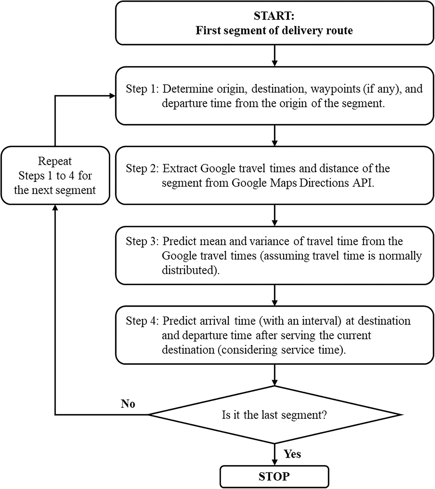
Figure 6: Procedure of the ATP algorithm for arrival time prediction

Step 1: Determine API parameters. The API parameters include the origin, destination, waypoints (if any), and departure time from the origin of the route segment.

Step 2: Extract the Google travel times (GTTs) and distance of the route segment. The API parameters, an access key, and a traffic model parameter are entered into a URL domain of the Google Maps Directions API. The URL domains are deployed for requesting the optimistic and pessimistic GTTs and the distance of the route segment.

Step 3: Predict the mean and variance of travel time by applying the SD technique. The mean and variance of predicted travel time are determined by the expressions in Eqs. (5) and (3), respectively.

Step 4: Predict arrival time (with an interval) at the destination and departure time after service by applying the ST and LT techniques. The prediction process in step uses Eqs. (7) to (12) and (14).

The process will repeat from Steps 1 to 4 for the next route segment and will stop at the last route segment.

3.4 Communication and Data Sharing System

The CDS system deploys smartphones with mobile signals, Internet access, Google Maps, Google Drives, Google Sheets, Line, and Telegram for communicating and sharing information among employees (CS, IT, planner, drivers) and customers. The planner needs a computer to efficiently manage information among stakeholders. Note that Email is needed for formal procedure and compliance purposes.

The CDS system is implemented for various stages of delivery services as follows (Fig. 2):

•   A customer, CS staff, and IT staff can share the delivery location by using Line and Telegram. Then, the IT staff can pinpoint the exact delivery location by using Google Maps and record it in a Google Sheet.

•   The planner can share (1) the delivery list and delivery schedule (Google Sheet link) and (2) a delivery route map (Google My Maps link) with each driver via Line and Telegram for driver’s feedback and executing delivery services.

•   The planner can inform the predicted interval of arrival time to each customer via a phone call, SMS in Line and Telegram, etc.

•   The drivers can view the delivery route maps and navigate the direction of a route segment using Google Maps on smartphones.

4  An Application of the Developed DMS System

This section presents the implementation of the DSM system to a Thai Small to Medium Enterprise (SME) that owns a delivery fleet of pickup trucks for providing delivery services in Section 4.1. Then, it discusses the experimental results in Section 4.2.

4.1 Implementation of the DSM System

A real experiment was conducted by implementing the proposed Delivery Service Management (DSM) system to manage the delivery services of an adhesive manufacturer in Bangkok, Thailand. The business process and the implementation of the proposed DSM system are presented in Fig. 2.

The typical business process of SMEs for fulfilling the orders of customers is described as follows. First, the Customer Service (CS) staff receives a Purchase Order (PO) from a customer via phone calls, line apps, emails, etc. The CS staff creates a Sales Order (SO) for each PO in the accounting database of the company. Second, the storekeeper picks the products from the storage area and packs them according to the SO for delivery on the next day. Third, the Finance staff creates a bill in the accounting database and confirms the billing with the customer. Fourth, the planner manages the delivery fleet to deliver products to customers. Note that most planner of SMEs manually-intuitively prepares the delivery plans of vehicles based on individual knowledge and experience. Finally, each driver delivers products and bills to customers starting in the morning of the next day.

The adhesive company was selected due to the following reasons. First, the adhesive company is a Thai SME that has similar characteristics to most SMEs in emerging countries. It has around 60 employees and about THB 200 million (USD 6 million) in annual sales. Second, the Thai SME owns a delivery fleet of four pickup trucks and hires permanent drivers to operate the fleet. It provides delivery services of many adhesive products to many Business-to-Business (B2B) customers located in Bangkok and its vicinity. The pickup trucks have to travel through the whole road network which has various traffic conditions. Third, the company often receives orders from new customers that have no historical delivery data. Fourth, the planner who manages the delivery fleet is not a technical expert. However, the planner has a bachelor’s degree and long working experience across various functions in the company. Therefore, this Thai SME is a suitable company for the application of the proposed DSM system.

The empirical parameters are estimated from the preliminary data of 140 delivery routes (including 814 customers served) collected from historical data of GPS tracking systems, manual records on delivery lists, and driver interviews. First, the maximum allowance and allowance reduction rate of travel time were estimated by using the linear regression equation between the error of travel time and travel distance. The maximum allowance and allowance reduction rate are the constant (5 min) and slope (−0.5 min/km) of the regression equation, respectively. We applied these same values to all route segments. Second, the estimated service time was the average of 814 service times (12 min). From the meetings with drivers and the management team, we have aligned to give additional 3 min as the allowance of service time (25% of service time). We assumed the same predicted service time (15 min) for all customers. Finally, lunchtime was the average value of 76 lunchtimes of drivers(20 min). We assumed the same lunch duration for all drivers. Note that for swift implementation of the proposed DSM system, the authors assume the same service time for all customers and the same lunch duration for all drivers. However, these parameters can be updated to be more accurate and robust after obtaining a large amount of data.

4.2 Results and Discussion

This section discusses the process perspective of the DLP and DRP systems and then analyzes the performance of the ATP system.

From the process perspective, the delivery services have become organized and effective after the implementation of the DSM system. The DSM system can improve the capability of SME employees. First, the DLP system adopted from [16] allows the customer service staff to have a clear procedure for obtaining completed and correct information from customers when receiving purchase orders. The DLP system has minimized the error of delivery locations. It eliminated the unnecessary tasks of drivers to call customers asking for the exact delivery locations during the day of delivery.

Second, the DRP system allowed the planner to plan more reliable routes by using the interface of Google My Maps (GMM) and waypoints compared to the current practice of the company. The DRP system has saved the planner time from working overnight to completing the delivery plan for the next delivery day. Moreover, the delivery plan provided the sequence of customers to be served such that the drivers can save unloading time from double handling.

From Fig. 4, the waypoints were added to the GMM interface for adjusting a realistic delivery route. The distance of the delivery route increased from 177 to 188 km, approximately 6% longer than the distance of the delivery route suggested by the GMM interface. However, the planned delivery route was a realistic one following the actual driving route and avoiding restricted road segments. This also improved the accuracy of the ATP system because of the accurate inputs of travel times.

The DRP system applied the CFRS concept. However, unlike the CFRS heuristics in [10,11], it used the GMM interface and waypoints as proposed in [16] to construct a realistic delivery route for each truck. The DRP system provides clear visibility of each delivery route. It is a better version of the HDS system proposed by [3] that did not have the visibility of a realistic route.

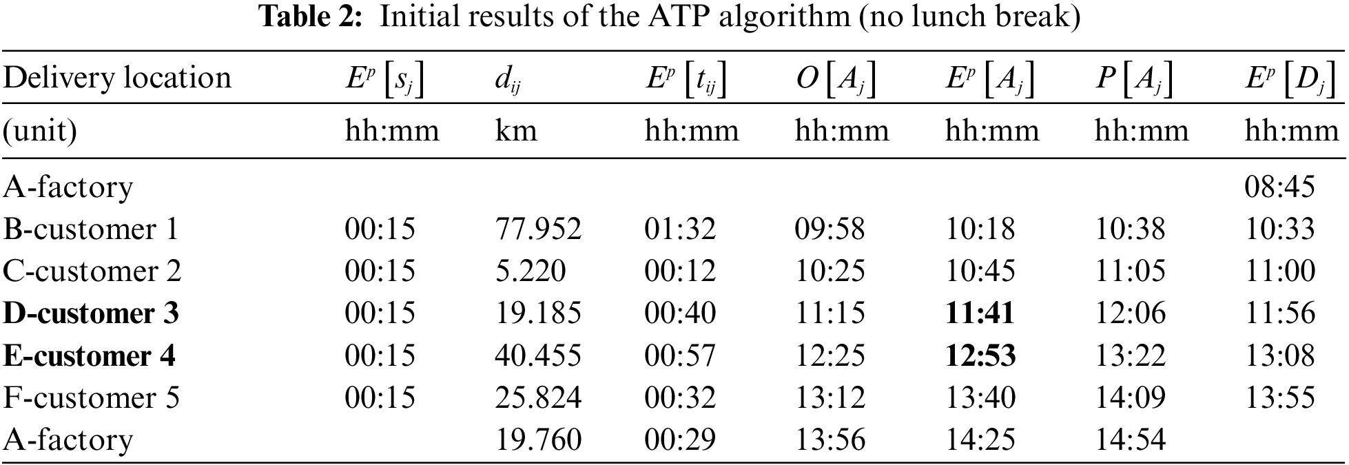
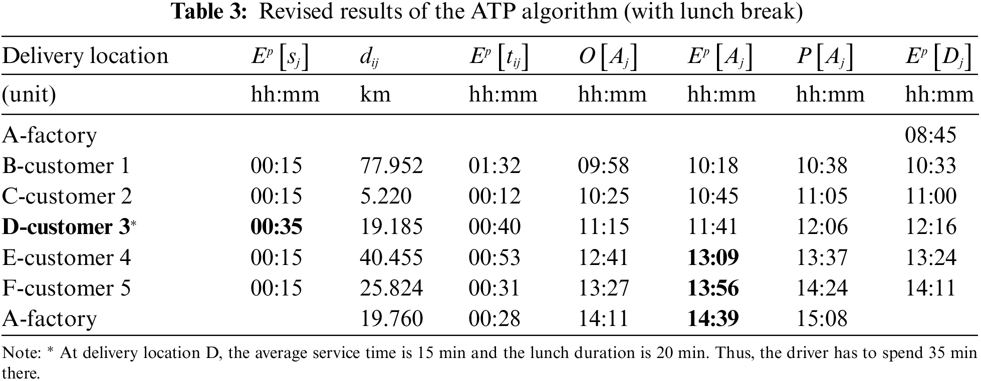
Third, the numerical example of the ATP system based on the delivery route in Fig. 4 is presented as follows. When the ATP system deploys the ATP algorithm with the SD and ST techniques, the results of arrival time prediction are shown in Table 2. From Table 2, the delivery truck passes through the route segment (D, E) during the lunchtime window [11:50,13:10]. By applying the LT technique, the delivery location D is selected as the lunch location and the predicted lunchtime is 20 min (see Eq. (13)). Then, including the lunchtime of 20 min, the ATP system deploys the ATP algorithm again. The results (illustrated in Table 3) show that when the LT technique is applied, it updates the predicted arrival times of customers that are served after the lunch break (see nodes E, F, and A).

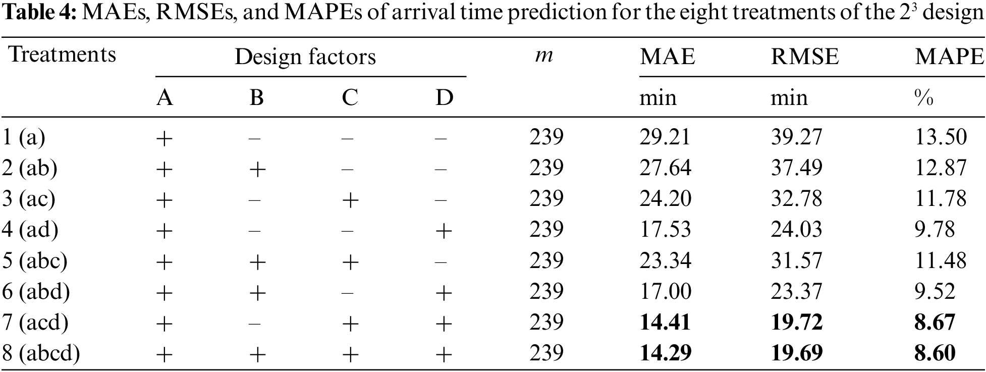
To analyze the impact of the ATP algorithm with the three techniques, the data of forty-one delivery routes have been collected from the delivery routes of four drivers. In total, 239 customers have been served. From the data, the effects of the ATP algorithm without and with the three proposed techniques (SD, ST, and LT) are evaluated.

Let factor A denotes the ATP algorithm that purely uses Google Maps API data for arrival time prediction. Factors B, C, and D denote SD, ST, and LT techniques, respectively. The sign (+) denotes the presence of a factor, and the sign (−) denotes the absence of a factor, respectively. The response variable is the absolute error of arrival time at each delivery location.

The 2k design is adapted for the experiment, where k=3 for factors B, C, and D, 23=8 treatment combinations, and m=239 replicates (Montgomery & Runger, 2014, pp. 581–600) [50]. Each treatment denotes an ATP algorithm that applies the presented factor(s) to predict arrival time. The summary of the treatment combinations for the experiment with the 23 design is shown in Table 4. Note that factor A has a presence in all treatments because the ATP algorithm using Google Maps API data is compulsory.

The Mean Absolute Error (MAE), Root-Mean-Square Error (RMSE), and Mean Absolute Percentage Error (MAPE) are used as measures for the accuracy of the ATP algorithms. The MAE and RMSE measure the average magnitude of errors in the ATP algorithms. The MAE gives equal weight to all individual errors, but the RMSE gives a relatively high weight to large errors. The MAPE measures the average percentage of errors. The MAE, RMSE, and MAPE are defined as the expressions in Eqs. (15)–(17), respectively.

Note that the departure time at the depot Ep[D0] is different from one delivery route to another. Before measuring the MAPE, the actual arrival time R[Aj] and predicted arrival time Ep[Aj] at each delivery location j must be normalized by subtracting Ep[D0] from both R[Aj] and Ep[Aj]. The experimental results are discussed as follows.

MAE=1m∑j=1m|Ep[Aj]−R[Aj]|(15)

RSME=1m∑j=1m(Ep[Aj]−R[Aj])2(16)

MAPE=1m∑j=1m|Ep[Aj]−R[Aj]R[Aj]−Ep[D0]|×100%(17)

The effects of three techniques (SD, ST, and LT) on the ATP algorithm are analyzed by using ANOVA with the General Linear Model (GLM) in Minitab 16 (see Table 5). From Table 5, two techniques (ST and LT) have significant effects on the absolute error of arrival time (p-value ≈0.000). The SD technique and two- and three-way interactions do not have a significant effect (p-value >0.05). Fig. 7 illustrates the plot of the main effects of SD, ST, and LT techniques on the absolute error of arrival time. It shows that the ST and LT techniques can significantly reduce the MAE of arrival time. The SD technique also reduces the MAE of arrival time, but it is not statistically significant. The effect of the SD technique may be insignificant because the number of road segments with a short distance is limited (approximately 20% of all segments). If more road segments are short distances, the effect of the SD technique may be significant.

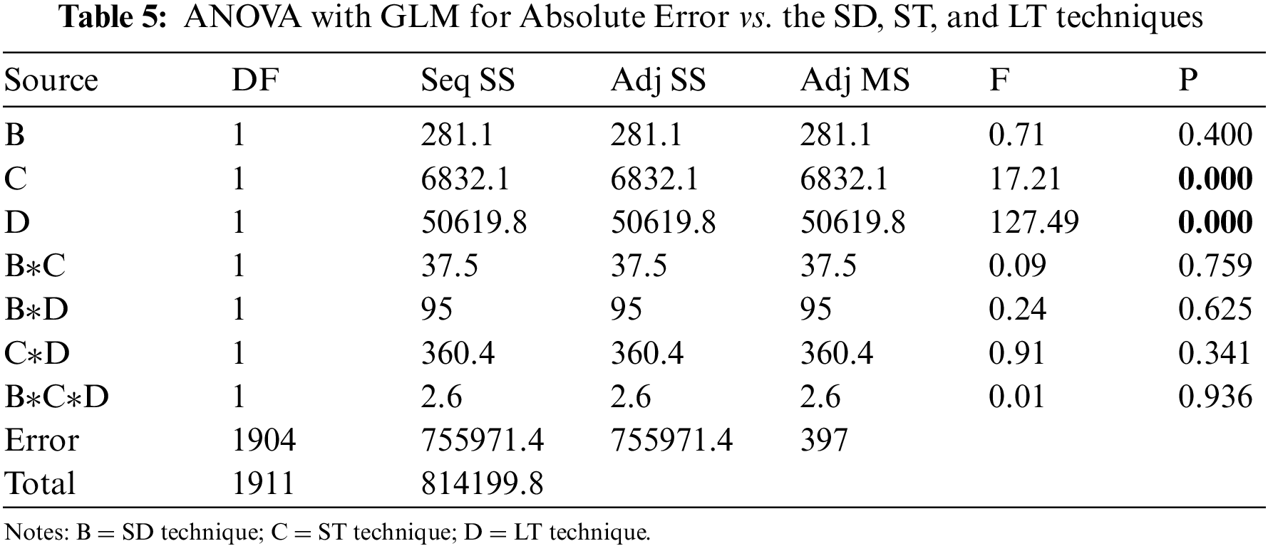
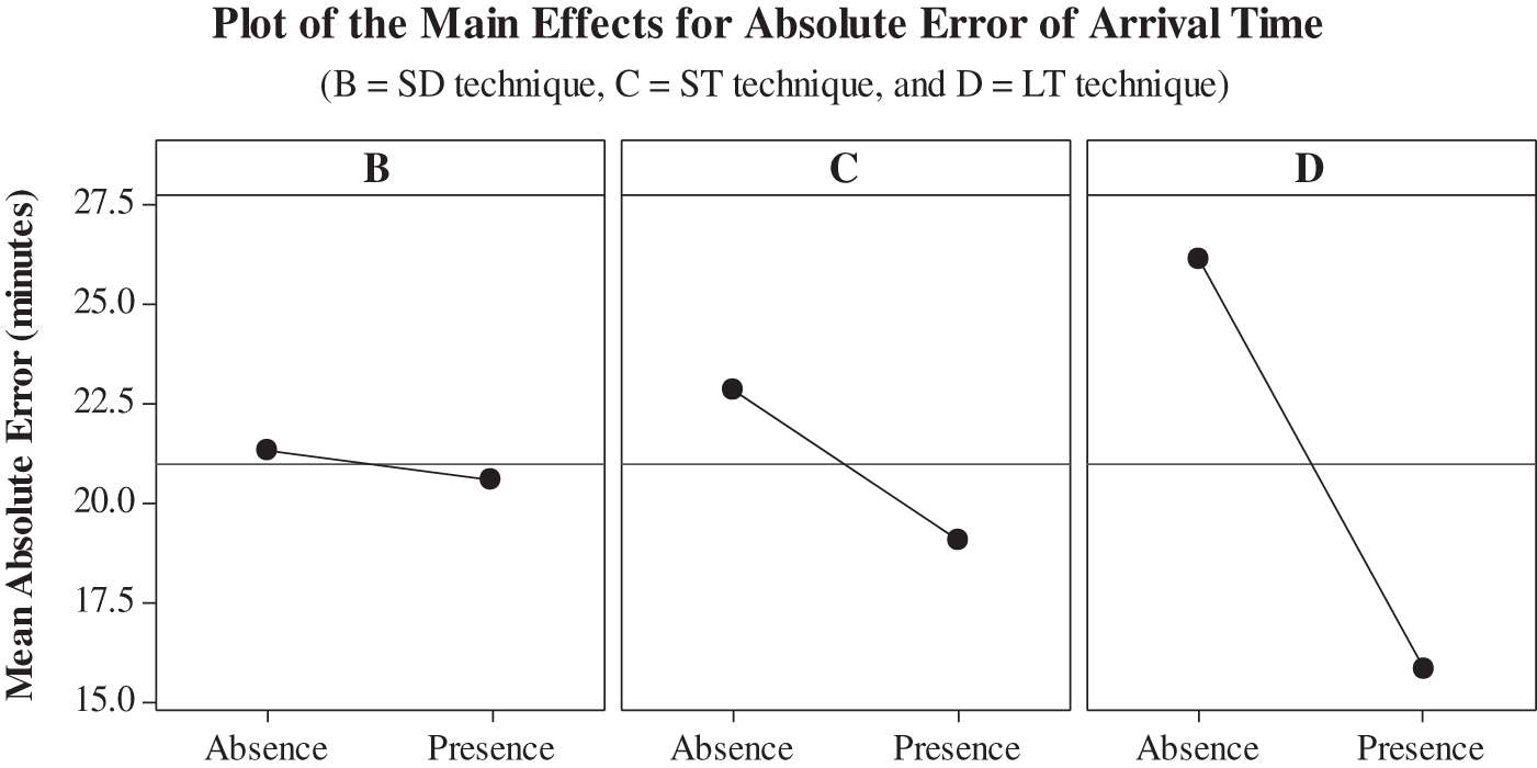
Figure 7: Plot of the main effects of SD, ST, and LT techniques for absolute error of arrival time

The MAE, RMSE, and MAPE are measures of the accuracy of the ATP algorithms. From Table 4, the ATP algorithm without the three techniques (Treatment 1), provides the highest values of MAE, RMSE, and MAPE with 29.21 min, 39.27 min, and 13.50%, respectively. In contrast, the ATP algorithm with the three proposed techniques (Treatment 8), provides the lowest values of all three measures with 14.29 min, 19.69 min, and 8.60%, respectively. Therefore, the three proposed techniques significantly improve the accuracy of the ATP algorithms.

Fig. 8 illustrates the scatterplot of the Absolute Error (AE) and Absolute Percentage Error (APE) vs. arrival time. It shows that when arrival time is farther in the future, the AE increases but the APE decreases. This indicates that the errors of arrival time tend to accumulate to a certain extent but not purely accumulate. The errors in arrival time may be positive or negative and may cancel each other. Normally, arrival time is a summation of travel times and service times; thus, it is purely accumulated.

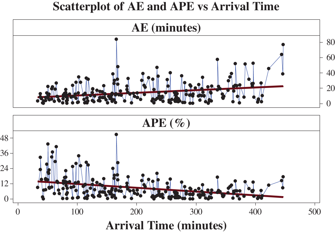
Figure 8: Scatterplot of Absolute Error (AE) and Absolute Percentage Error (APE) vs. arrival time

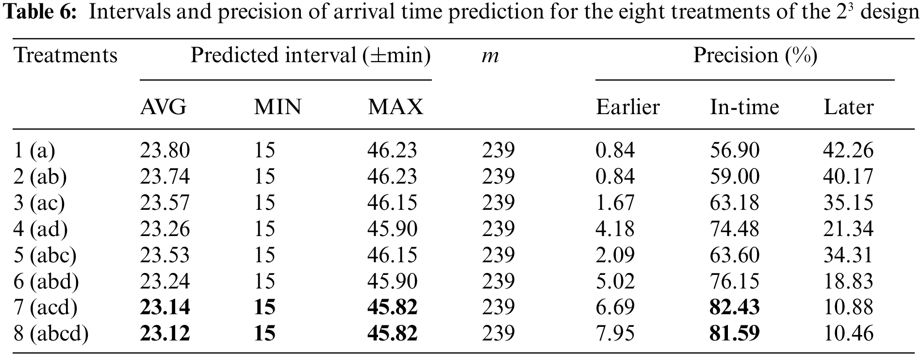
The intervals of the predicted arrival time measure the precision of the ATP algorithms. The ATP algorithm considers only the uncertainty of travel time. Therefore, the variation in arrival time that is accumulated results from the variations in travel time. The intervals of predicted arrival time are similar for all ATP algorithms (see Table 6). From Table 6, the average, minimum, and maximum values of the predicted intervals for the ATP algorithms are about ±23, ±15, and ±46 min, respectively. For the ATP algorithm without the three techniques (Treatment 1), 56.90% of actual arrival times are within the predicted intervals. This means that in only 56.90% of the delivery locations that the delivery trucks arrive there within the intervals predicted by the ATP algorithm without the three techniques. For the ATP algorithm with the three techniques (Treatment 8), 82.43% of actual arrival times are within the predicted intervals. The latter ATP algorithm provides higher delivery precision than the former one. Thus, the ATP algorithm with the three techniques is reliable, and it can enhance customer satisfaction with delivery services.

Similar to the studies in [29,31,41,46], the ATP system can provide the predicted arrival time (with an interval) at each customer. However, the proposed ATP system performed better than the existing studies as follows. First, the ATP system includes the whole road network for predicting the arrival time at each customer, while existing studies focused on freeways, highways, and bus routes. Second, the ATP system can predict the arrival time of each truck at each customer in future periods up to 8 h ahead. This is better than [29] which can predict travel time in future periods up to 1 h ahead.

5  Conclusions and Recommendations

This paper presented a Delivery Service Management (DSM) system for managing SME delivery services. The DSM system takes into account the limited capability of SME employees who involve with delivery services. The DSM system is proposed to identify the delivery locations of customers, plan the delivery route of each truck, predict arrival time at each delivery location, and communicate and share information among stakeholders.

The DSM system integrates four systems as follows: (1) Delivery Location Positioning (DLP), (2) Delivery Route Planning (DRP), (3) Arrival Time Prediction (ATP), and (4) Communication and Data Sharing (CDS) systems. These systems use IoT technologies, Cloud Computing, and simple applications as supporting tools. The supporting tools include a GPS tracking system, Google Maps, Google Maps APIs, Google Drives, Google Sheets, ATP algorithms embedded in Excel Macros (Excel VBA), and messenger applications (Line and Telegram).

This paper has significant contributions as follows. First, the proposed DSM system has been implemented to manage the delivery services of a Thai SME. It supports SME employees to eliminate unnecessary tasks from delivery services. The DSM system allows the planner to easily adjust delivery routes using a “waypoint” so that the planned and actual routes are the same. Most commercial software generates a planned route that is difficult to be adjusted to be the same as the actual route. When the planned and actual routes are the same, it eliminates confusion for the planner, driver, and customers. Moreover, the arrival time prediction will be more accurate since it is calculated from the realistic planned route which is the same as the actual route.

Second, the proposed ATP system utilizes three proposed techniques related to driver behaviors for arrival time prediction. These techniques include compensation for short-distance travel time (SD), allowance for a short rest after service (ST), and lunch location-time estimation (LT). Based on the experimental results of the case study, the effects of the ST and LT techniques are significant but the effect of the SD technique is not significant. This result is very useful for developing an accurate ATP system. We suggest that all ATP systems should consider a location to take lunch and the lunch duration of a driver (LT technique); otherwise, the arrival time to customers after lunch will be inaccurate. When the delivery requires the driver to move many units of considerable weight goods to a stock room of the customer, the driver will have fatigue and usually requires a rest time before driving the truck to the next customer. In this situation, the ST technique that considers a short rest time for the driver after serving the customer is recommended.

Third, based on experimental results the ATP algorithm with the SD, ST, and LT techniques is reliable enough that approximately 82% of actual arrival times fall within the estimated intervals of arrival times, where the average, minimum, and maximum values of the predicted intervals are about ±23, ±15, and ±46 min, respectively. The numerical results may be dependent on the dataset of this company. When the proposed system is applied to other SMEs with different datasets, the absolute values of the results may be changed. The estimated parameters used in the experiment, for example, the service time at each customer and the lunch duration of each driver, are case-dependent. When these parameters of other companies are longer than the parameters of this company, the effect of the proposed techniques related to driver behaviors will be more significant. It is expected that the performance of the proposed system is still acceptable and the stakeholders’ experiences are still good.

The limitations of the proposed DSM system and recommendations for further study are provided as follows. First, the DRP system used the experience of the planner and drivers to construct each delivery route. An efficient DRP system may deploy machine learning such as Artificial Intelligence (AI) and image processing to auto-suggest delivery routes and auto-adjust route segments to avoid restricted road segments and traffic congestion. Second, the ATP system used normal distribution assumptions for travel time and empirical values for input parameters. The improved ATP system should consider the availability of big data in cloud databases and use data science techniques to get insightful assumptions and more reliable values of input parameters. Third, the experimental case study did not monitor the delivery status of the fleet of pickups in real time. A Delivery Truck Monitoring (DTM) system that allows the planner to monitor the position and delivery status of each truck in real time should be implemented. The DTM system can adapt the real-time interface of the GPS tracking system. When an accident or unexpected delay happens, the planner can detect it sooner. Then if the delay impacts the arrival times of the truck at other customers of the route, the planner can revise the delivery plan and share it with the driver and remaining customers for acknowledgment.

Acknowledgement: The authors would like to thank the owners and employees of the company, and senior project teams who supported this research during the preliminary and experimental implementation processes. The authors would like to thank the reviewers who provide constructive comments to improve the quality of the submitted manuscript.

Funding Statement: The authors received no specific funding for this study.

Conflicts of Interest: The authors declare that they have no conflicts of interest to report regarding the present study.

References

1. M. D. Ismail and S. S. Alam, “Innovativeness and competitive advantage among small and medium enterprise exporters: Evidence from emerging markets in South East Asia,” The South East Asian Journal of Management, vol. 13, no. 1, pp. 74–91, 2019. [Google Scholar]

2. G. Habault, Y. Taniguchi and N. Yamanaka, “Delivery management system based on vehicles monitoring and a machine-learning mechanism,” in Proc. 2018 IEEE 88th Vehicular Technology Conf. (VTC-Fall), Chicago, IL, USA, pp. 1–5, 2018. [Google Scholar]

3. A. Kandakoglu, A. Sauré, W. Michalowski, M. Aquino, J. Graham et al., “A decision support system for home dialysis visit scheduling and nurse routing,” Decision Support Systems, vol. 130, no. 1, pp. 113224, 2020. [Google Scholar]

4. P. Lacomme, G. Rault and M. Sevaux, “Integrated decision support system for rich vehicle routing problems,” Expert Systems with Applications, vol. 178, no. 1, pp. 114998, 2021. [Google Scholar]

5. K. Braekers, K. Ramaekers and I. van Nieuwenhuyse, “The vehicle routing problem: State of the art classification and review,” Computers & Industrial Engineering, vol. 99, no. 1, pp. 300–313, 2016. [Google Scholar]

6. M. Gendreau, G. Ghiani and E. Guerriero, “Time-dependent routing problems: A review,” Computers & Operations Research, vol. 64, no. 1, pp. 189–197, 2015. [Google Scholar]

7. C. Lin, K. L. Choy, G. T. S. Ho, S. H. Chung and H. Y. Lam, “Survey of green vehicle routing problem: Past and future trends,” Expert Systems with Applications, vol. 41, no. 4, pp. 1118–1138, 2014. [Google Scholar]

8. R. Fukasawa, Q. He and Y. Song, “A branch-cut-and-price algorithm for the energy minimization vehicle routing problem,” Transportation Science, vol. 50, no. 1, pp. 23–34, 2016. [Google Scholar]

9. G. Marques, R. Sadykov, J. C. Deschamps and R. Dupas, “An improved branch-cut-and-price algorithm for the two-echelon capacitated vehicle routing problem,” Computers & Operations Research, vol. 114, no. 1, pp. 104833, 2020. [Google Scholar]

10. S. E. Comert, H. R. Yazgan, S. Kır and F. Yener, “A cluster first-route second approach for a capacitated vehicle routing problem: A case study,” International Journal of Procurement Management, vol. 11, no. 4, pp. 399–419, 2018. [Google Scholar]

11. S. Horng and P. Yenradee, “Performance comparison of two-phase LP-based heuristic methods for capacitated vehicle routing problem with three objectives,” Engineering Journal, vol. 24, no. 5, pp. 145–159, 2020. [Google Scholar]

12. S. F. Ghannadpour and A. Zarrabi, “Multi-objective heterogeneous vehicle routing and scheduling problem with energy minimizing,” Swarm and Evolutionary Computation, vol. 44, no. 1, pp. 728–747, 2019. [Google Scholar]

13. Y. Marinakis, M. Marinaki and A. Migdalas, “A multi-adaptive particle swarm optimization for the vehicle routing problem with time windows,” Information Sciences, vol. 481, no. 1, pp. 311–329, 2019. [Google Scholar]

14. D. Sedighizadeh and H. Mazaheripour, “Optimization of multi objective vehicle routing problem using a new hybrid algorithm based on particle swarm optimization and artificial bee colony algorithm considering precedence constraints,” Alexandria Engineering Journal, vol. 57, no. 4, pp. 2225–2239, 2018. [Google Scholar]

15. H. Zhang, Q. Zhang, L. Ma, Z. Zhang and Y. Liu, “A hybrid ant colony optimization algorithm for a multi-objective vehicle routing problem with flexible time windows,” Information Sciences, vol. 490, no. 1, pp. 166–190, 2019. [Google Scholar]

16. S. Horng and P. Yenradee, “Delivery location positioning and delivery planning systems for Thai SMEs using google maps,” in Proc. Int. Multi-Conf. on Advances in Engineering, Technology, and Management (IMC-AEMT 2020), Bangkok, Thailand, pp. 102–107, 2020. [Google Scholar]

17. P. Kirci, “A novel model for vehicle routing problem with minimizing CO2 emissions,” in Proc. 2019 3rd Int. Conf. on Advanced Information and Communications Technologies (AICT), Lviv, Ukraine, pp. 241–243, 2019. [Google Scholar]

18. L. Santos, J. Coutinho-Rodrigues and C. H. Antunes, “A web spatial decision support system for vehicle routing using google maps,” Decision Support Systems, vol. 51, no. 1, pp. 1–9, 2011. [Google Scholar]

19. J. Muniz de Miranda Sá and M. Maghrebi, “A more realistic approach towards concrete delivery dispatching problem: Using real distance instead spatial distance,” Australian Journal of Civil Engineering, vol. 16, no. 1, pp. 1–11, 2018. [Google Scholar]

20. A. K. Beheshti, S. R. Hejazi and M. Alinaghian, “The vehicle routing problem with multiple prioritized time windows: A case study,” Computers & Industrial Engineering, vol. 90, no. 1, pp. 402–413, 2015. [Google Scholar]

21. V. Baradaran, A. Shafaei and A. H. Hosseinian, “Stochastic vehicle routing problem with heterogeneous vehicles and multiple prioritized time windows: Mathematical modeling and solution approach,” Computers and Industrial Engineering, vol. 131, no. 1, pp. 187–199, 2019. [Google Scholar]

22. D. Lee and J. Ahn, “Vehicle routing problem with vector profits with max-min criterion,” Engineering Optimization, vol. 51, no. 2, pp. 352–367, 2019. [Google Scholar]

23. P. Alvarez, I. Lerga, A. Serrano-Hernandez and J. Faulin, “The impact of traffic congestion when optimising delivery routes in real time. A case study in Spain,” International Journal of Logistics Research and Applications, vol. 21, no. 5, pp. 529–541, 2018. [Google Scholar]

24. Y. Huang, L. Zhao, T. van Woensel and J. -P. Gross, “Time-dependent vehicle routing problem with path flexibility,” Transportation Research Part B: Methodological, vol. 95, no. 1, pp. 169–195, 2017. [Google Scholar]

25. U. Mori, A. Mendiburu, M. Álvarez and J. A. Lozano, “A review of travel time estimation and forecasting for advanced traveller information systems,” Transportmetrica A: Transport Science, vol. 11, no. 2, pp. 119–157, 2015. [Google Scholar]

26. S. Mil and M. Piantanakulchai, “Modified Bayesian data fusion model for travel time estimation considering spurious data and traffic conditions,” Applied Soft Computing, vol. 72, no. 1, pp. 65–78, 2018. [Google Scholar]

27. E. -H. Chung and A. Shalaby, “Expected time of arrival model for school bus transit using real-time global positioning system-based automatic vehicle location data,” Journal of Intelligent Transportation Systems, vol. 11, no. 4, pp. 157–167, 2007. [Google Scholar]

28. E. J. Schmitt and H. Jula, “On the limitations of linear models in predicting travel times,” in Proc. 2007 IEEE Conf. on Intelligent Transportation Systems, Bellevue, WA, USA, pp. 830–835, 2007. [Google Scholar]

29. R. Li and G. Rose, “Incorporating uncertainty into short-term travel time predictions,” Transportation Research Part C: Emerging Technologies, vol. 19, no. 6, pp. 1006–1018, 2011. [Google Scholar]

30. G. Chen, X. Yang, J. An and D. Zhang, “Bus-arrival-time prediction models: Link-based and section-based,” Journal of Transportation Engineering, vol. 138, no. 1, pp. 60–66, 2012. [Google Scholar]

31. Z. Yu, J. S. Wood and V. V. Gayah, “Using survival models to estimate bus travel times and associated uncertainties,” Transportation Research Part C: Emerging Technologies, vol. 74, no. 1, pp. 366–382, 2017. [Google Scholar]

32. Y. Zhou, L. Yao, Y. Chen, Y. Gong and J. Lai, “Bus arrival time calculation model based on smart card data,” Transportation Research Part C: Emerging Technologies, vol. 74, no. 1, pp. 81–96, 2017. [Google Scholar]

33. W. Fan and Z. Gurmu, “Dynamic travel time prediction models for buses using only GPS data,” International Journal of Transportation Science and Technology, vol. 4, no. 4, pp. 353–366, 2015. [Google Scholar]

34. B. Yu, W. H. K. Lam and M. L. Tam, “Bus arrival time prediction at bus stop with multiple routes,” Transportation Research Part C: Emerging Technologies, vol. 19, no. 6, pp. 1157–1170, 2011. [Google Scholar]

35. Y. Bin, Y. Zhongzhen and Y. Baozhen, “Bus arrival time prediction using support vector machines,” Journal of Intelligent Transportation Systems, vol. 10, no. 4, pp. 151–158, 2006. [Google Scholar]

36. J. Wang and Q. Shi, “Short-term traffic speed forecasting hybrid model based on chaos-wavelet analysis-support vector machine theory,” Transportation Research Part C: Emerging Technologies, vol. 27, no. 1, pp. 219–232, 2013. [Google Scholar]

37. B. A. Kumar, L. Vanajakshi and S. C. Subramanian, “Bus travel time prediction using a time-space discretization approach,” Transportation Research Part C: Emerging Technologies, vol. 79, no. 1, pp. 308–332, 2017. [Google Scholar]

38. M. Altinkaya and M. Zontul, “Urban bus arrival time prediction: A review of computational models,” International Journal of Recent Technology and Engineering, vol. 2, no. 4, pp. 164–169, 2013. [Google Scholar]

39. H. Min and E. Melachrinoudis, “Melachrinoudis A model-based decision support system for solving vehicle routing and driver scheduling problems under hours of service regulations,” International Journal of Logistics Research and Applications, vol. 19, no. 4, pp. 256–277, 2016. [Google Scholar]

40. A. Bezuglov and G. Comert, “Short-term freeway traffic parameter prediction: Application of grey system theory models,” Expert Systems with Applications, vol. 62, no. 1, pp. 284–292, 2016. [Google Scholar]

41. X. Fei, C. -C. Lu and K. Liu, “A Bayesian dynamic linear model approach for real-time short-term freeway travel time prediction,” Transportation Research Part C: Emerging Technologies, vol. 19, no. 6, pp. 1306–1318, 2011. [Google Scholar]

42. M. Yildirimoglu and N. Geroliminis, “Experienced travel time prediction for congested freeways,” Transportation Research Part B: Methodological, vol. 53, no. 1, pp. 45–63, 2013. [Google Scholar]

43. Y. Zou, X. Zhu, Y. Zhang and X. Zeng, “A space-time diurnal method for short-term freeway travel time prediction,” Transportation Research Part C: Emerging Technologies, vol. 43, no. 1, pp. 33–49, 2014. [Google Scholar]

44. N. Julio, R. Giesen and P. Lizana, “Real-time prediction of bus travel speeds using traffic shockwaves and machine learning algorithms,” Research in Transportation Economics, vol. 59, no. 1, pp. 250–257, 2016. [Google Scholar]

45. D. Sun, H. Luo, L. Fu, W. Liu, X. Liao et al., “Predicting bus arrival time on the basis of global positioning system data,” Transportation Research Record: Journal of the Transportation Research Board, vol. 2034, no. 1, pp. 62–72, 2007. [Google Scholar]

46. D. Woodard, G. Nogin, P. Koch, D. Racz, M. Goldszmidt et al., “Predicting travel time reliability using mobile phone GPS data,” Transportation Research Part C: Emerging Technologies, vol. 75, no. 1, pp. 30–44, 2017. [Google Scholar]

47. A. Gal, A. Mandelbaum, F. Schnitzler, A. Senderovich and M. Weidlich, “Traveling time prediction in scheduled transportation with journey segments,” Information Systems, vol. 64, no. 1, pp. 266–280, 2017. [Google Scholar]

48. H. Yu, D. Chen, Z. Wu, X. Ma and Y. Wang, “Headway-based bus bunching prediction using transit smart card data,” Transportation Research Part C: Emerging Technologies, vol. 72, no. 1, pp. 45–59, 2016. [Google Scholar]

49. C. P. I. van Hinsbergen, J. W. C. van Lint and H. J. van Zuylen, “Bayesian committee of neural networks to predict travel times with confidence intervals,” Transportation Research Part C: Emerging Technologies, vol. 17, no. 5, pp. 498–509, 2009. [Google Scholar]

50. D. C. Montgomery and G. C. Runger, Applied Statistics and Probability for Engineers, 6th ed., Hoboken, NJ, USA: John Wiley & Sons, 2014. [Google Scholar]