Fractional Processing Based Adaptive Beamforming Algorithm

1  Introduction

Smart antennas use the spatial domain to improve wireless communication systems by providing greater coverage and higher data rates through spatial diversity in a multipath channel environment. They are widely used in wireless communication, radar, sonar, navigation, and tracking systems [1–4]. They improve performance and capacity while requiring no additional spectrum allocation. Smart antennas are used to improve signal quality and spectral efficiency whereas reducing system power consumption. They estimate the direction of arrival (DOA) [5,6] of signals and use beamforming techniques [7] to cancel out signals from undesirable directions and receive signals from preferred directions. Signal processing techniques used in antenna arrays and beamforming techniques are summarized in references [8,9]. Adaptive beamforming is a form of beamforming that uses algorithms to adjust the weights applied to incoming signals in real-time, allowing the beam to change dynamically in response to changes in the environment. This provides better performance in dynamic and complex environments compared to fixed beamforming. Fig. 1 depicts its block diagram.

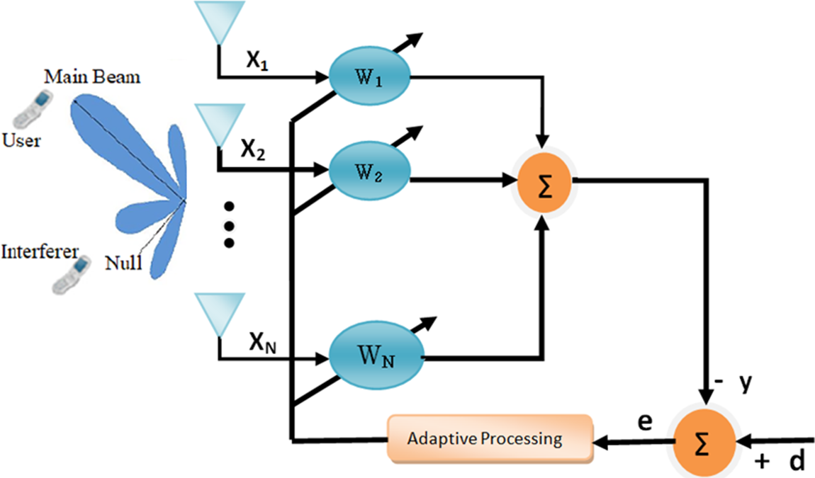
Figure 1: Adaptive beamforming block diagram

Smart antenna systems rely on adaptive algorithms to make the necessary adjustments for system efficiency. These algorithms are classified as either non-blind or blind. Training signals are available for weight adaptation in non-blind algorithms. In the literature, adaptive algorithms such as least mean square (LMS) [10], recursive least square (RLS) [11], constant modulus algorithm (CMA) [12], and others are used for beamforming. Combined LMS-LMS (LLMS) [13] and RLS-LMS (RLMS) [14] are two-stage algorithms for adaptive array beamforming that demonstrate fast convergence and high accuracy on the cost of complexity. LLMS consists of two concatenated sections of LMS, whereas in RLMS, RLS and LMS sections are separated by array image factor. In [15], a Kalman-based parallel RLMS algorithm is proposed, showing stability with a moderate increase in complexity even for lower signal-to-interference noise ratios (SINR). The LMS algorithm is widely used in antenna array beamforming due to its fast signal tracking, simplicity, and robustness. However, LMS has slow convergence, which has prompted several modifications [16–19]. A variable step size least mean square (VSS-LMS) algorithm, for example, is proposed in [16], with the step size determined by a normalized sigmoid function. In [17] authors presented a two-stage LLMS algorithm for concentric circular arrays. The two-stage parallel LMS [18] reduces complexity and provides ease in hardware implementation. The DMI-RLS algorithm consisting of direct matrix inversion and recursive least square algorithm stages proposed [20]. The algorithm based on conventional beamforming [21] directs the beam in the desired direction and places nulls in the interferer’s direction to minimize interference. The preferred algorithms have a good balance between convergence speed, signal tracking, complexity, stability, and robustness. Beamforming is a popular and continuously researched area in various fields, including 5G wireless communications [22], medical imaging [23], and networks [24]. The reader can find more stuff by consulting the research works listed in [25–34].

Fractional calculus is a relatively new area of research that has been gaining attention for its applications in various fields of engineering [35–38]. It has been applied in image processing [39], control systems [40], circuit analysis [41], channel tracking [42], and more. Fractional calculus-based algorithms have shown better performance in various applications such as channel equalization [43–45], recommender systems [46], noise control [47–49], line echo control [50], and beamforming [51]. In [52], the author has proved the superiority of fractional order processing for different signal processing applications over standard algorithms. The fractional LMS algorithm has also been used for system identification [53] and power signal modeling [54]. The use of fractional calculus in differential equations has also been demonstrated in [55–57]. Fractional calculus implementation is reported in wireless sensor networks [58]. Overall, fractional processing-based algorithms have been shown to perform well compared to standard algorithms [59–65]. Authors are motivated by the success of fractional signal processing in various other fields and believe that it can improve the performance of adaptive beamforming algorithms. Enabling the use of fractional order derivatives can provide greater flexibility in weight parameter adaptation. The fractional order algorithm is a new approach for adaptive array beamforming that uses a combination of standard and fractional order derivatives. The input to the algorithm is the signals received at the uniform linear array [66] elements which are contaminated by noise and interfering signals. The algorithm updates the weight vector of the FLMS using an error obtained by the difference of the desired and output signal. The performance of the algorithm is evaluated using Matlab simulation results, which consider various parameters such as the number of array elements, step size, SNR, and fractional order. The algorithm is compared with the standard LMS algorithm using metrics such as MSE convergence speed, scatter plots, and beam pattern accuracy. In Fig. 2 block diagram of proposed model is presented.

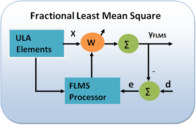
Figure 2: Fractional least mean square adaptive beamforming model

This paper’s organization describes that in Section 2, a system model for FLMS-based adaptive beamforming and the convergence analysis of the FLMS are presented. Section 3 includes results from Matlab simulations and discussions. The final section, Section 4, provides conclusions and suggestions for future work.

2  General Description of Proposed Model (FLMS)

This section of the paper models the adaptive array beamforming system using the proposed FLMS algorithm. The beamformer in the model receives desired and interfering signals from various directions and impinges on L evenly spaced isotropic ULA components from M distant sources. The element spacing is half the wavelength of the signal, and the direction of arrival (DOA) of the targeted and interfering signals is assumed to be known, otherwise it can be estimated by other algorithms [6,26,67–70].

The FLMS algorithm is a non-blind algorithm used for beamforming that aims to estimate the optimal weights for the received signals (X) to produce the desired output (y) using Eq. (6). The reference signal (d) is available and is used to calculate the error (e) between the output (y) and reference signal (d). The error is then used to adjust the weight vector to converge the algorithm. The performance of the algorithm is evaluated using the mean square error (MSE) because of its mathematical tractability.

For the proposed algorithm, some assumptions are made, such as the system environment being stationary and the input signals being statistically independent. Further signals are assumed to be uncorrelated and to have a zero mean.

2.1 Mathematical Model

In this setup of adaptive array beamforming, the signal array vector is composed of binary phase shift keying (BPSK) signal received at array elements and is represented by the transposed vector:

X=[x1,x2,x3,…xM]T(1)

The desired and interfering signals are random and drawn from uniform, independent, and identical distributions. The signal array vector may be represented as a combination of desired and interfering signals in the element form given by:

X=Sd(n)a(θd)+∑0L−1Si(n)a(θi)+b(n)(2)

Here Sd is the desired signal, and Si is the interfering signal. a(θd) and a(θi) are the steering vectors for desired and interfering signals, respectively. θd and θi are the angles of arrival of the desired and interferer signals respectively. Here b is white Gaussian noise.

Taking the first array element as a reference, the steering vectors are represented as follows:

a(θd)=[1,e−jψd,e−j2ψd…e−jLψd]T(3)

a(θi)=[1,e−jψi,e−j2ψi…e−jLψi]T(4)

In this equation, ψd=2πDλsinθd and ψi=2πDλsinθi are the inter-element phase shifts with respect to desired and interfering signals respectively, [.]T represents transpose, D corresponds to antenna element spacing and λ is the wavelength of the signal.

Weight W is applied to the input signal (X) on every iteration, and summed, yielding the output of the algorithm y:

y=WHX(5)

Where W=[w1,w2,w3,…wL]T(6)

The array factor for ULA is given as:

AF(θd)=∑n=1L⁡ej(n−1)ψd(7)

In this equation, ψd=2πDλsinθd is the inter element phase shift.

2.2 Least Mean Square Algorithm

The cost function J(n) for LMS, which is based on the MSE minimization criterion is expressed as:

J(n)=E[{e(n)}2]=E[{d(n)−y(n)}2](8)

By putting Eq. (5) and rearranging, Eq. (8) becomes:

J(n)=d2(n)+WHX(n)WHX(n)−2d(n)WHX(n)(9)

The equation for the updated weight vector is given using an iterative approach by differentiating the cost function for LMS

W(n+1)=W(n)+μ∂J(n)∂W(10)

or

W(n+1)=W(n)+μe(n)X(n)(11)

Here W is the weight vector, μ is the step size, e is the error signal, and X is the input signal.

2.3 Fractional Least Mean Square (FLMS) Algorithm

It is a modified LMS that employs fractional order derivatives along with standard order derivatives in the weight adaptation of LMS. The cost function for LMS is the mean square error minimization in Eq. (8) and its weight update equation given in Eq. (10):

J(n)=E[{e(n)}2]=E[{d(n)−y(n)}2]

W(n+1)=W(n)+∂J(n)∂W

The weight update equation for the FLMS has both the standard order and fractional order derivatives, given as:

W(n+1)=W(n)−[μ∂J(n)2∂W+μ∂∝J(n)2∂∝W](12)

Here ∝ is the fractional order whereas μ is the step size.

By definition of fractional order derivative of f(t)=Xn:

D∝f(t)=∂∝f(t)∂∝W=Γ(m+1)Γ(m−∝+1)Xn−∝(13)

D∝=∂∝∂∝W: is the ∝ order fractional derivative operator

Γ: is the gamma function

Γ(z)=∫0∞tz−1e−tdt(14)

By taking the cost function’s fractional order derivative with respect to W:

∂∝∂∝WJ(n)=−2(e(n)X(n−k))D∝W(n)(15)

Putting D∝=∂∝∂∝W and using Eq. (12) in Eq. (14) results into:

∂∝∂∝WJ(n)=−2(e(n)X(n−k))1Γ(2−∝)x1−∝(16)

By taking the standard order derivative of the cost function:

∂J(n)∂W=−2e(n)X(n−k)(17)

Using Eqs. (16) and (17), finally the updated weight equation of Eq. (10), in vector form is written as:

W(n+1)=W(n)+μe(n)X(n)+μe(n)X(n)⊙1Γ(2−∝)W1−∝(18)

Here ⨀ represents the element by element multiplication.

2.4 Fractional Least Mean Square Algorithm (Caputo Derivative)

In the weight vector adaptation, FLMS employs fractional in addition to standard order derivatives. The cost function J(n) and weight update equation for LMS are given in Eqs. (8) and (10), respectively:

J(n)=E[{e(n)}2]

W(n+1)=W(n)−∂J(n)∂W

The error signal is estimated as:

e(n)=d(n)−y(n)(19)

The algorithm’s output is given by the equation below:

y(n)=W(n)X(n)(20)

The weight vector given in Eq. (11) is as follows:

W(n+1)=W(n)+μe(n)X(n)

The weight update equation in FLMS contains both the standard and fractional order derivatives. It’s because the incoming signal is a Gaussian process. The weight update equation is:

W(n+1)=W(n)−μ∂J(n)∂W−μ∂∝J(n)∂W∝(21)

The fractional order ∝ value is 0<∝<1. Because of its complexity, engineering approximation is employed in place of the chain rule, asD∝e2=e(n)D∝e(n). After taking an integer order derivative, the equation becomes:

W(n+1)=W(n)−μe(n)X(n)−μ∂∝J(n)∂W∝(22)

Once a fractional order derivative is applied, the weight update equation becomes:

W(n+1)=W(n)+μe(n)X(n)+μe(n)X(n)⊙1Γ(2−∝)W1−∝(23)

Here ⨀ represent the element-by-element multiplication

2.5 Convergence Analysis of FLMS

The received signal consists of desired, interfering, and noise signals. When weights are applied to this input signal, an output signal is produced. Input (X) and weight (W) vectors are given in Eqs. (1) and (6), respectively are:

W=[w1,w2,w3,…xL]

X=[x1,x2,x3,…xM]T

LMS weight updates equation as given in Eq. (11) is:

W(n+1)=W(n)+μe(n)X(n)(24)

The weight updates equation for FLMS as given in Eq. (23) is:

W(n+1)=W(n)+μe(n)X(n)+μe(n)X(n)⊙1Γ(2−∝)W1−∝(25)

Some other frame of reference is employed to reveal the properties of convergence of FLMS. The error vector v′ can be expressed as follows:

v′(n)=W(n)−Wo(26)

Here Wo is the optimal weight vector, to cancel out the effects of the interfering signal. The error signal obtained using the optimal weight is:

eo(n)=d(n)−XT(n)Wo(27)

Error vector in the next instant (n+1) is given by the equation:

v′(n+1)=W(n+1)−Wo(28)

For LMS it becomes:

v′(n+1)=W(n)+μe(n)XT(n)−Wo(29)

After putting v′(n)=W(n)−Wo we get:

v′(n+1)=v′(n)+μe(n)XH(n)(30)

After substitutions and rearranging Eq. (30) results in:

v′(n+1)=v′(n)+μXH(n)(eo(n)+XT(n)Wo−XT(n)W(n))(31)

In simplified form, it can be written as:

v′(n+1)=v′(n)+μXH(n)(eo(n)+XT(n)v′(n))(32)

After applying the orthogonality principle, this vector simplifies to:

v′(n+1)=[I−μ(n)R]v′(n)(33)

After pre-multiplying by a unitary matrix QT the equation becomes:

QTv′(n+1)=QT[I−μ(n)R]v′(n)(34)

After putting R=QT∧Q, Eq. (34) becomes:

QTv′(n+1)=QT[I−μ(n)QT∧Q]v′(n)(35)

QTv′(n+1)=[I−μ(n)∧]QTv′(n)(36)

Here ∧ represents diagonal matrix of eigenvalues.

Suppose v(n)=QTv′(n) then the equation becomes:

v(n+1)=[I−μ(n)∧]v(n)(37)

For FLMS weight vectors consider μi=Γ(2−∝)μ keeping it simple:

W(n+1)=W(n)+μe(n)X(n)+μe(n)X(n)⊙W(n)1−∝(38)

For column vector I of ones, the equation can be written as follows:

W(n+1)=W(n)+μe(n)X(n)+[I+I⊙W(n)1−∝](39)

When the statistical independence expectation and orthogonality principle are applied to both sides, the equation becomes:

E[v(n+1)]=[I−μR+μR⊙E[|v(n)|1−∝]]E[v(n)](40)

Eq. (40) can be written as:

E[v(n+1)]=[I−μR(I−I⊙E[∖v(n)|1−∝])]E[v(n)](41)

Replacing I⨀E[|v(n)|1−∝] by F(W(n),∝) the equation becomes:

E[v(n+1)]=[I−μR(I−F(W(n),∝)]E[v(n)](42)

At a stable state, the mean power of the weight difference should decrease as the number of iterations increases, we have:

limn→∞‖E[v(n)]‖2=0(43)

It is only possible for −1<I−μR(I−F(W(n),∝)<1. After simplification, it is written as I<μ<2R−F(W(n),∝).

It can also be represented in terms of eigenvalues λmax as follows:

I<μ<2λmax−F(W(n),∝)(44)

Eq. (44) offers a choice of step size selection for the convergence of a fractional algorithm. Additional nonlinear terms produced due to fractional processing provides ease in the adjustment of the correlation matrix so that even at larger step sizes improved convergence is ensured.

3  Simulations Environment

The simulations of the proposed algorithm use the setup and parameters listed in Table 1.

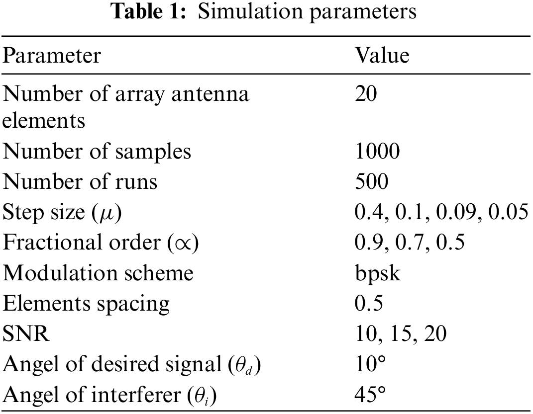
•   There are 20 isotropic array elements in ULA.

•   Element spacing is half the wavelength of the signal (d=0.5λ).

•   The desired BPSK modulated signal arrives at an angle of 10°.

•   The interfering BPSK modulated signal arrives at an angle of 45°.

•   Both desired and interfering signals are contaminated with Gaussian noise.

3.1 Simulation Results and Discussion

The simulations evaluate a fractional order adaptive beamforming algorithm using Monte Carlo simulations. The simulations test the algorithm’s performance under different signal-to-noise ratio (SNR), fractional order, and step size conditions. The evaluation is based on the comparison of mean square error (MSE) learning curves and convergence rates for 1000 samples and 500 independent runs. The desired signal has a direction of arrival (DOA) of 10°, while the interfering signal has a DOA of 45°. Fig. 3 illustrates the flow chart of the model. The simulation results are presented in various figures with comparisons between the FLMS and LMS algorithms. The evaluation of the proposed algorithm’s performance is based on MSE convergence speed, beampattern accuracy and scatter plots. Fig. 4 compares the MSE convergence speed for FLMS and LMS algorithms. Similarly, plots in Figs. 5 to 8 examine the MSE learning curves of the suggested approach for varying SNR, step size, and fractional order values. Fig. 9 depicts the beampattern performance of the FLMS and LMS. The performance of the scatter plot for FLMS and LMS is compared in Fig. 10 at the end. In these findings, step sizes are denoted by μ(mu) while fractional order is denoted by ∝ (nu).

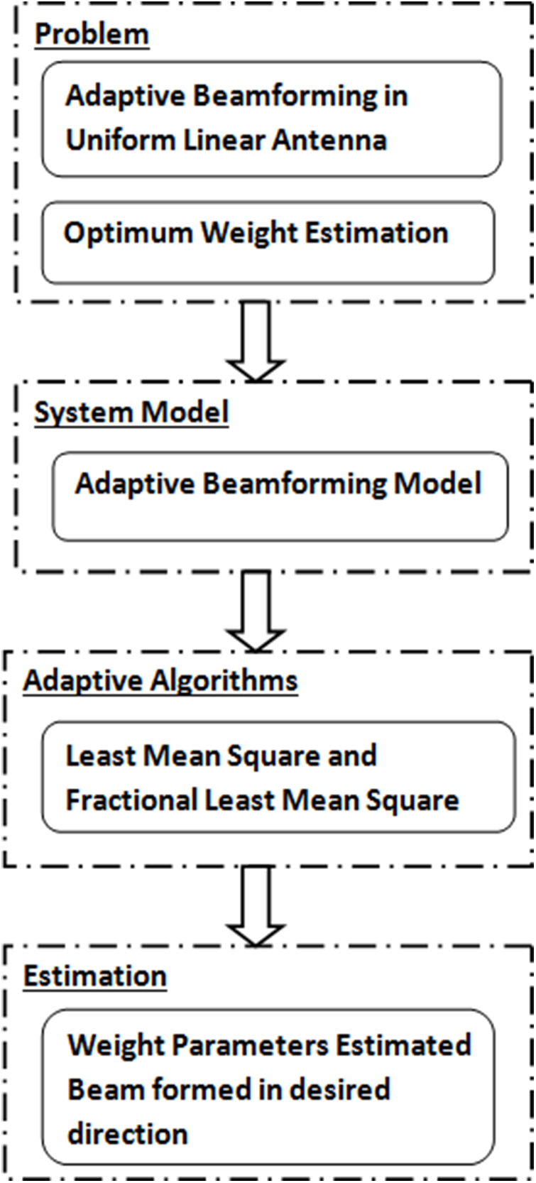
Figure 3: Flow chart of proposed model

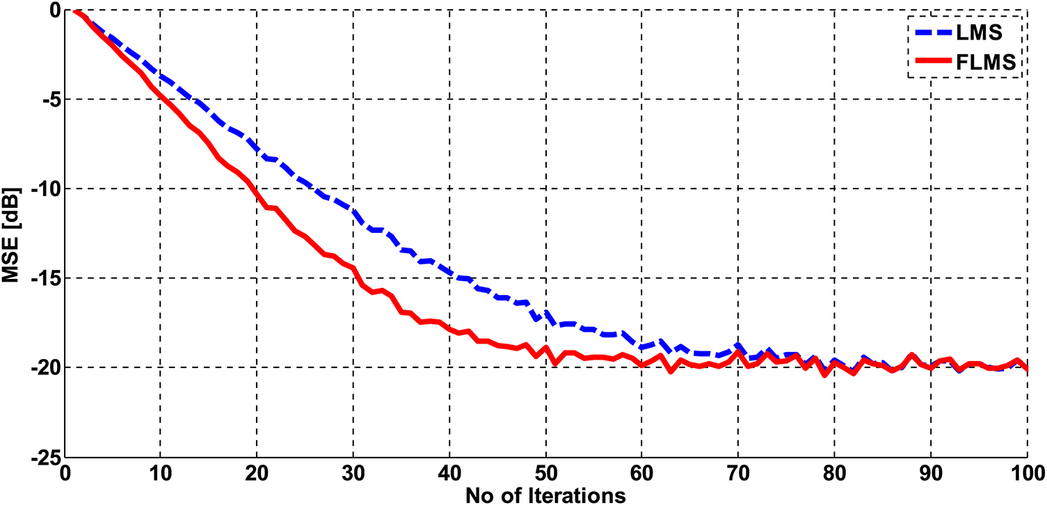
Figure 4: MSE convergence performance of LMS and FLMS

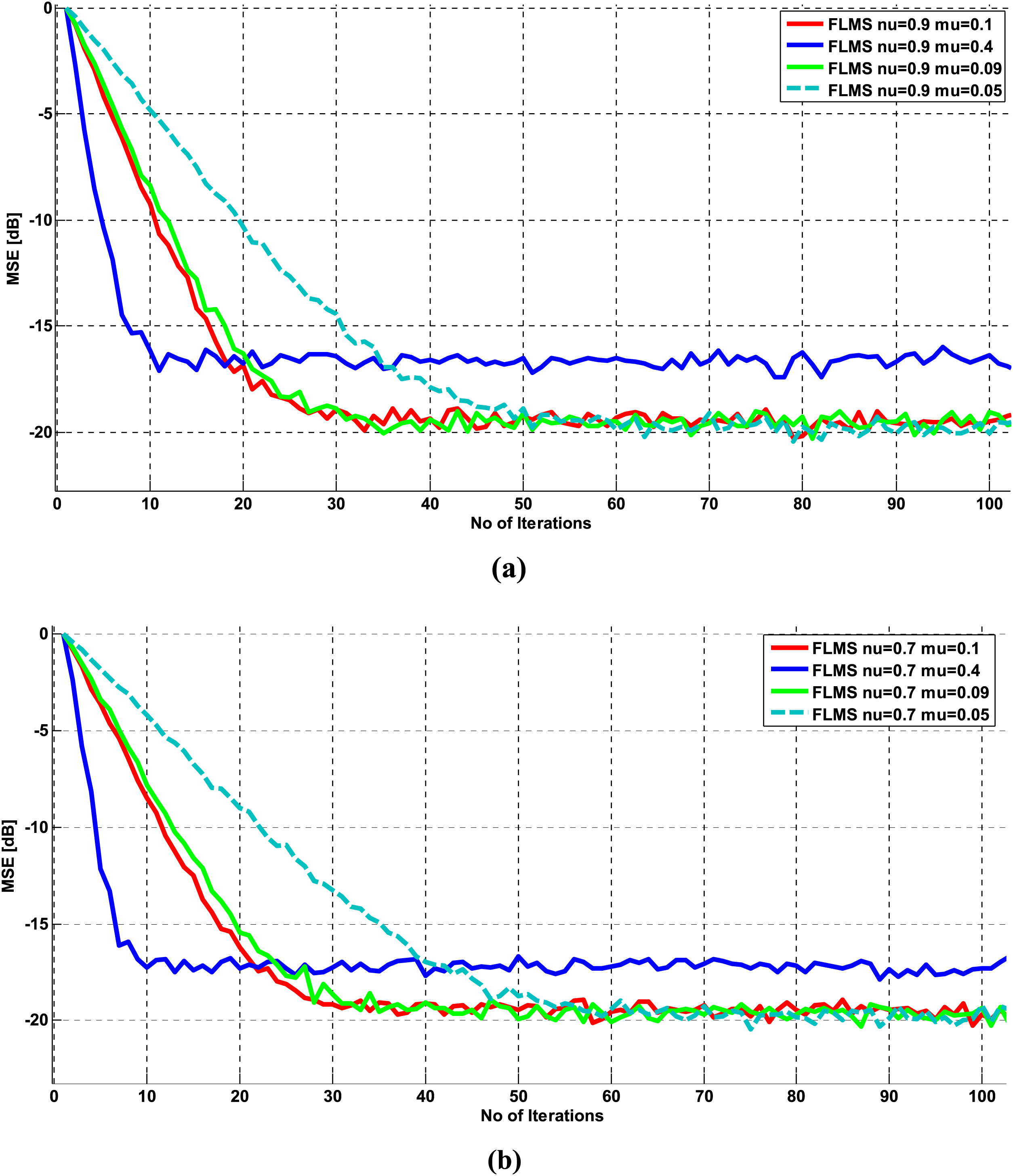
Figure 5: FLMS MSE learning curves for SNR = 10 and for various values of step size (a) ∝ = 0.9 (b) ∝ = 0.7

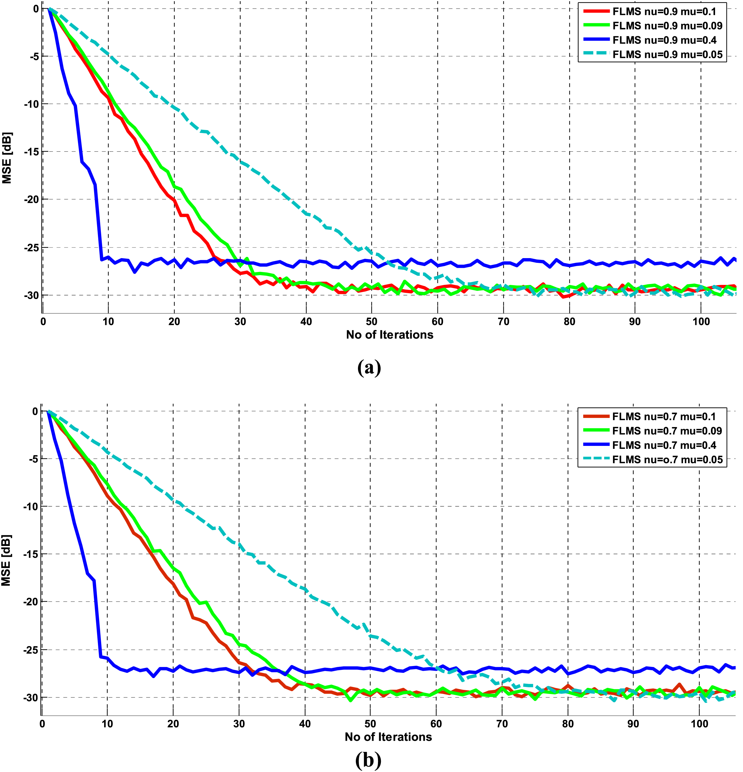
Figure 6: FLMS MSE learning curves for SNR = 15 for various values of step size µ (a) ∝ = 0.9 (b) ∝ = 0.7

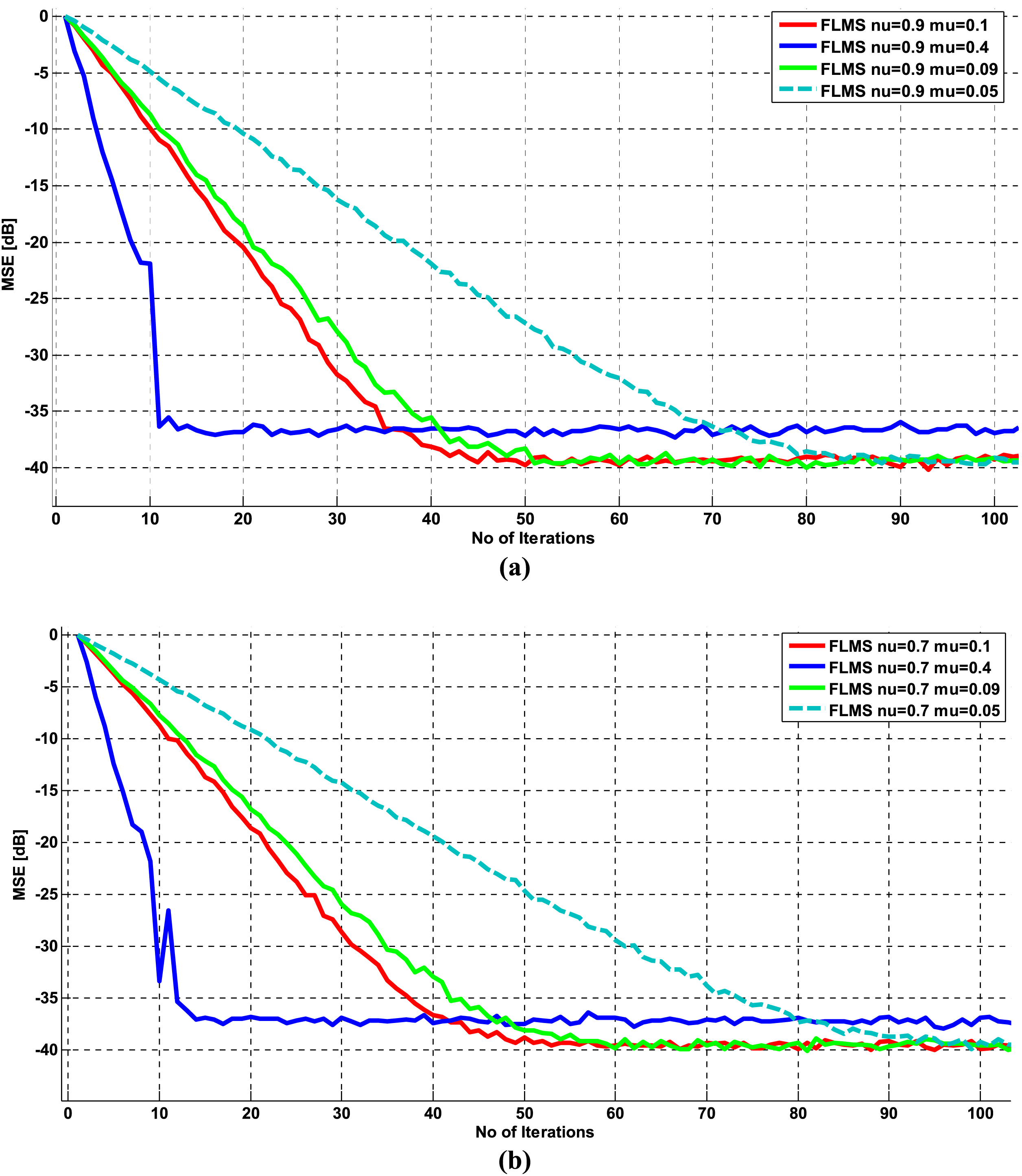
Figure 7: FLMS MSE learning curves for SNR = 20 for various values of step size µ (a) ∝ = 0.9 (b) ∝ = 0.7

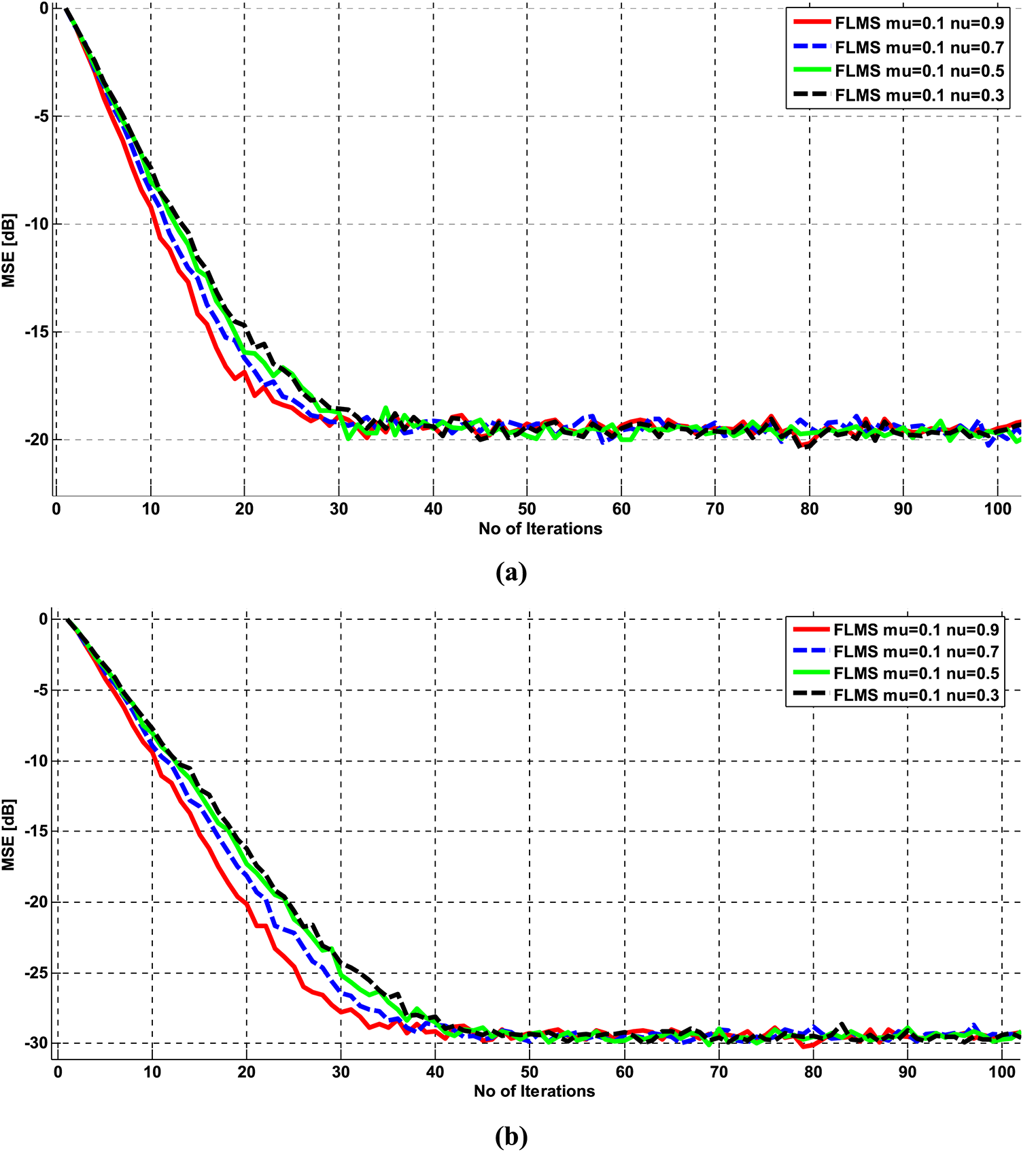
Figure 8: FLMS MSE learning curves (a) SNR 10, µ = 0.1, various fractional orders (b) SNR = 15, µ=0.1, various fractional orders

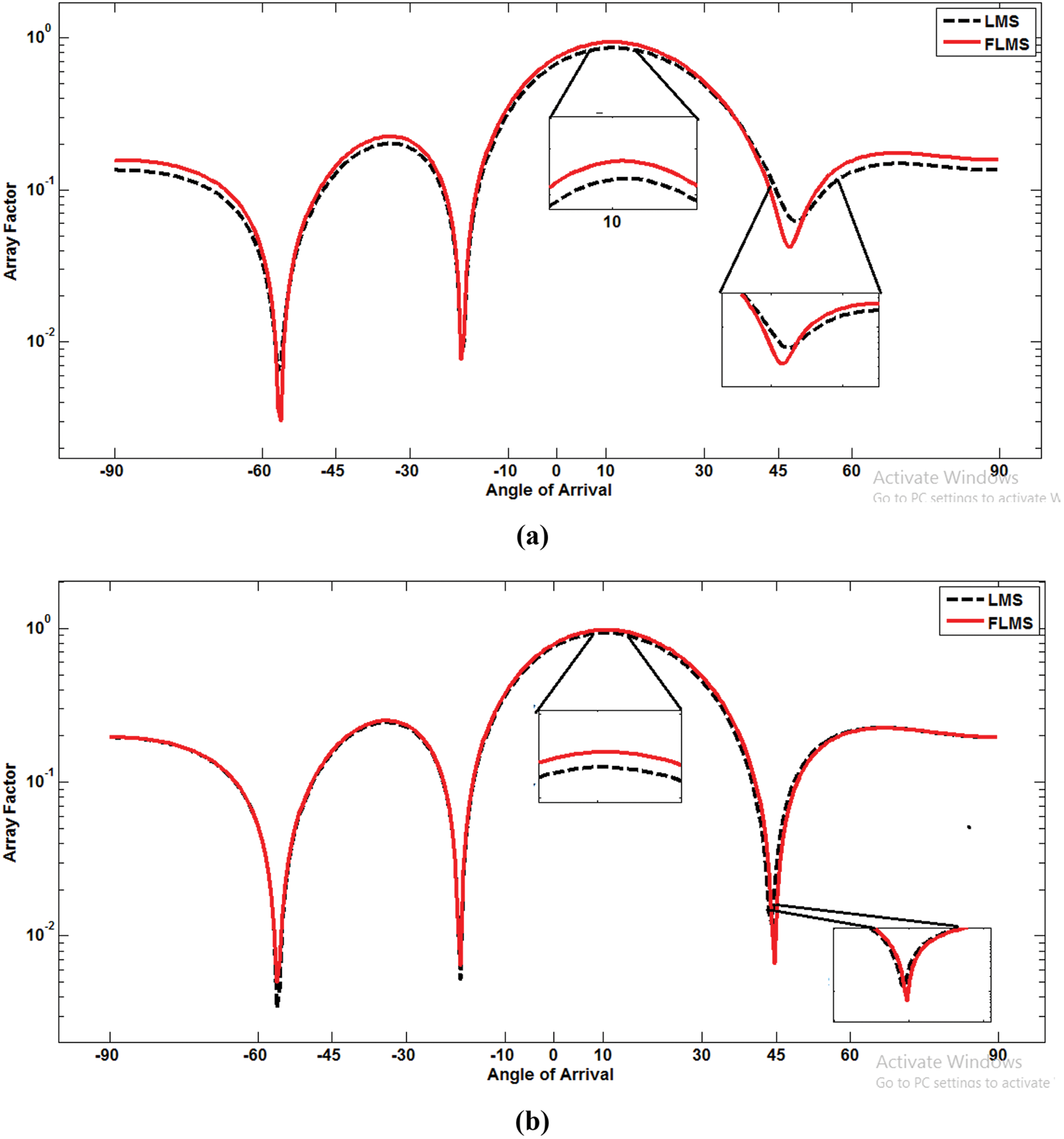
Figure 9: (a) Beam pattern SNR = 10, ∝ = 0.9, μ = 0.05, (b) beam pattern SNR = 15, ∝ = 0.9, μ = 0.01

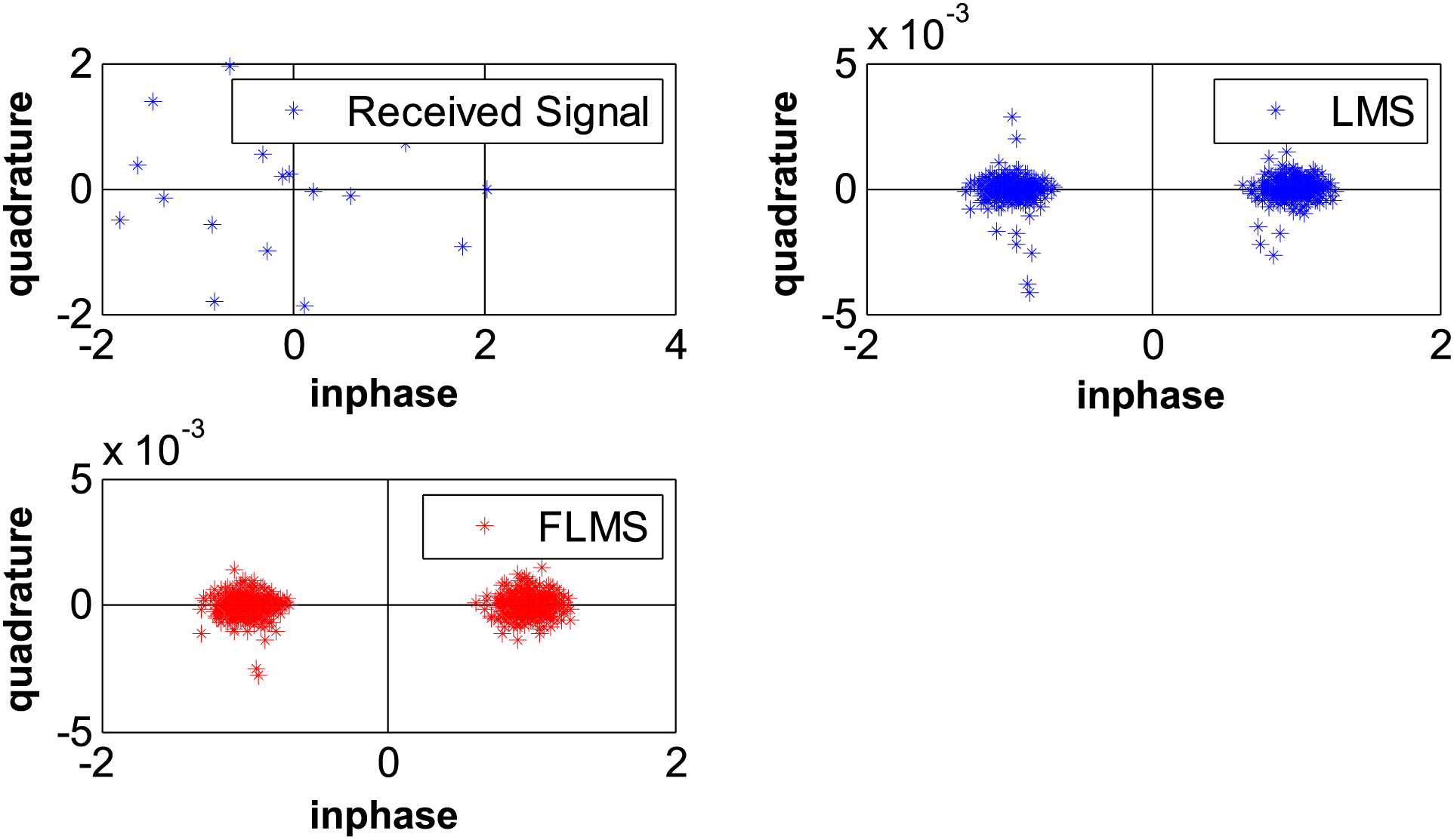
Figure 10: Scatter plots comparison for FLMS and LMS

3.1.1 MSE Convergence Performance

The results in Fig. 4 demonstrate that when SNR is 10 dB, μ is 0.05, and ∝ is 0.9, the fractional least mean square algorithm has a faster convergence rate compared to the least mean square algorithm. Specifically, FLMS reaches a mean squared error (MSE) value of −20 dB at the 51st iteration, while LMS reaches the same value at the 78th iteration. This corresponds to 34% improvement. Similarly for μ is 0.1 the convergence of FLMS occurs at the 33rd iterations while LMS converges at the 45th iteration. For SNR value of 15 dB, μ=0.1, and ∝=0.9, the fractional FLMS algorithm converges at 41st iteration whereas LMS at the 62nd iteration. The results establish FLMS provides better performance than the LMS algorithm.

3.1.2 MSE Performance of FLMS for Varying Step Sizes

The learning curves in Figs. 5a and 5b show the impact of varying step size on the mean squared error (MSE) performance of the fractional least mean squares algorithm. As the step size decreases, the steady-state MSE performance improves, but the convergence speed slows down. For example, in Fig. 5a, with a step size of μ = 0.4, the FLMS algorithm converges to −15 dB at the 8th iteration, while with μ = 0.1, it converges to −15 dB at the 17th iteration. The same pattern can be observed in Fig. 5b for a fractional order (∝ = 0.7) and varying step sizes.

The results shown in Figs. 6a and 6b for signal-to-noise ratio (SNR) of 15 dB indicate that the step size has an effect on the convergence rate and steady-state mean squared error (MSE) performance of the algorithm. Increasing the step size improves the convergence rate but degrades the steady-state MSE performance. When the SNR is increased, the overall steady-state MSE performance of the algorithm improves to −30 dB. The fastest convergence to −25 dB is achieved with a step size of μ = 0.4 at the 9th iteration, as shown in Fig. 6a. In Fig. 6b, the effect of varying step sizes on MSE convergence is shown for a fractional order of 0.7. The same pattern as in Fig. 6a is repeated, but with a slight decrease in convergence speed.

The mean squared error (MSE) performance for a signal-to-noise ratio (SNR) of 20 dB is evaluated and presented in Figs. 7a and 7b. The behavior is consistent with the results for SNR = 10 and SNR = 15, with an improved steady-state MSE performance that converges to −40 dB.

3.1.3 MSE Performance of FLMS for Varying Fractional Orders

The MSE performance is evaluated in Figs. 8a and 8b by keeping the SNR and step size constant while varying the fractional orders (0.9, 0.7, 0.5, 0.3). As shown in Fig. 8a, increasing the value of fractional order enhances the convergence speed. Increasing the SNR from 10 to 15 dB increases the convergence speed as depicted in Fig. 8b. Another point that can be concluded from these figures is that the steady-state MSE performance improves significantly converges to −30 dB for SNR = 15.

3.1.4 Beampatterns

The beampatterns in Fig. 9 demonstrate the accuracy of directing the main lobe beam in a desired direction (10°) and placing a null in the direction of an interfering signal (45°). Four antenna elements are used in these plots to show the difference obvious, as decreasing the number of antenna elements leads to an increase in the width of the lobes. Fig. 9a shows the beampatterns for SNR = 10, μ = 0.1, and ∝ = 0.9. The main beam of the fractional least mean squares (FLMS) algorithm is accurately directed at an angle of 10° and placed null at interferer angle of 45°, showing superior performance than the least mean squares (LMS) algorithm. Fig. 9b shows the results obtained for SNR = 15, μ = 0.1, and ∝ = 0.9, where again the FLMS algorithm performs better than the LMS algorithm.

3.1.5 Performance Evaluation in Terms of Scattered Plots

The scatter plot in Fig. 10 compares the performances of the fractional least mean squares (FLMS) algorithm and the least mean squares (LMS) algorithm for SNR = 10, ∝ = 0.9, and μ = 0.1. The plot shows that in terms of scatter plots, the FLMS algorithm performs well than the LMS algorithm for the same SNR, step size, and fractional orders. The scatter plots of the FLMS algorithm demonstrate higher precision and accuracy, with less spreading compared to the LMS algorithm.

4  Conclusions

Beamforming is an important feature of modern communication and radar systems. A fractional order adaptive algorithm is proposed for beamforming applications. The fractional-order adaptive beamforming (FLMS) algorithm was derived and simulated in this research work. A mathematical convergence analysis provided shows that the use of fractional derivatives in a system can improve its convergence and steady state response by reducing the spread of the autocorrelation matrix’s eigenvalues. This leads to better performance even with larger step sizes. The simulation results illustrate that FLMS outperforms the standard least mean square (LMS) algorithm in terms of MSE convergence speed by 34%. FLMS also showed better directivity and gain, resulting in improved coverage while reducing power consumption. The results indicate that FLMS has the potential to be applied in various categories of adaptive signal processing applications, i.e., system identification, inverse modeling, prediction, etc, and offer improved performance over traditional algorithms. In future work, the FLMS can be evaluated by changing various parameters, such as the number of array elements, the number of interferers, and different modulation schemes. Additionally, the fractional order approach can be extended to other adaptive filtering algorithms, such as RLS and NLMS, to evaluate their performance in adaptive beamforming applications. These lines of inquiry can provide new insights and potential avenues for improving the performance of adaptive beamforming algorithms.

Funding Statement: This work is supported by the Office of Research and Innovation (IRG project # 23207) at Alfaisal University, Riyadh, KSA.

Conflicts of Interest: The authors declare that they have no conflicts of interest to report regarding the present study.

References

1. G. Sun, Y. Liu, H. Li, J. Li, A. Wang et al., “Power-pattern synthesis for energy beamforming in wireless power transmission,” Neural Computing and Applications, vol. 30, no. 7, pp. 2327–2342, 2018. [Google Scholar]

2. W. Jin, W. Jia, F. Zhang and M. Yao, “A user parameter-free robust adaptive beamformer based on general linear combination in Tandem with steering vector estimation,” Wireless Personal Communications, vol. 75, no. 2, pp. 1447–1462, 2014. [Google Scholar]

3. S. Haykin, “Radar array processing for angle of arrival estimation,” in Array Signal Processing, 1st ed., vol. 1. Englewood Cliffs, NJ, USA: Prentice-Hall, pp. 194–242, 1985. [Google Scholar]

4. M. A. Gondal and A. Anees, “Analysis of optimized signal processing algorithms for smart antenna system,” Neural Computing and Applications, vol. 23, no. 3, pp. 1083–1087, 2013. [Google Scholar]

5. B. R. Jackson, S. Rajan, B. J. Liao and S. Wang, “Direction of arrival estimation using directive antennas in uniform circular arrays,” IEEE Transactions on Antennas and Propagation, vol. 63, no. 2, pp. 736–747, 2015. [Google Scholar]

6. M. Z. U. Khan, A. N. Malik, F. Zaman and I. M. Qureshi, “Robust LCMV beamformer for direction of arrival mismatch without beam broadening,” Wireless Personal Communications, vol. 104, no. 1, pp. 21–36, 2019. [Google Scholar]

7. J. Li and P. Stoica, “Robust capon beamforming,” in Robust Adaptive Beamforming, 1st ed., vol. 1. New Jersey, USA: John Wiley & Sons, pp. 91–200, 2005. [Google Scholar]

8. B. D. V. Veen and K. M. Buckley, “Beamforming: A versatile approach to spatial filtering,” IEEE ASP Magazine, vol. 5, no. 2, pp. 4–24, 1988. [Google Scholar]

9. J. A. Stine, “Exploiting smart antennas in wireless mesh networks using contention access,” IEEE Transaction on Wireless Communications, vol. 13, no. 2, pp. 38–49, 2006. [Google Scholar]

10. B. Widrow, J. M. McCool, M. G. Larimore and C. R. Johnson, “Stationary and nonstationary learning characteristics of the LMS-adaptive filter,” in Proc. IEEE, NY, USA, vol. 64, pp. 1151–1162, 1976. [Google Scholar]

11. F. Ling and J. G. Proakis, “Nonstationary learning characteristics of least squares adaptive estimation algorithm,” in Proc. IEEE ICASSP, San Diego, CA, USA, pp. 118–121, 1984. [Google Scholar]

12. D. N. Godard, “Self-recovering equalization and carrier tracking in two dimensional data communication systems,” IEEE Transaction on Communication, vol. 28, no. 11, pp. 1867–1875, 1980. [Google Scholar]

13. J. A. Srar, K. Chung and A. Mansour, “Adaptive array beamforming using a combined LMS-LMS algorithm,” IEEE Transactions on Antennas and Propagation, vol. 58, no. 11, pp. 3545–3557, 2010. [Google Scholar]

14. J. A. Srar and K. Chung, “Adaptive array beam forming using a combined RLS-LMS algorithm,” in Proc. 14th APCC, Akihabara, Japan, pp. 1–5, 2008. [Google Scholar]

15. G. Akkad, A. Mansour, B. Elhassan, J. A. Srar, M. Najem et al., “Low complexity robust adaptive beamformer based on parallel RLMS and Kalman RLMS,” in Proc. 27th EUSIPCO, A Coruna, Spain, pp. 1–5, 2019. [Google Scholar]

16. J. A. Srar, X. Yang, Q. Liu, T. Long and T. K. Sarkar, “Fast and robust variable-step-size LMS algorithm for adaptive beamforming,” IEEE Antennas and Wireless Propagation Letters, vol. 19, no. 7, pp. 1206–1210, 2020. [Google Scholar]

17. J. A. Srar, K. Chung and A. Mansour, “LLMS adaptive array beamforming algorithm for concentric circular arrays,” Advance Studies and Technology Letters (Signal Processing), vol. 37, pp. 65–77, 2013. [Google Scholar]

18. G. Akkad, A. Mansour, B. El-Hassan, E. Inaty, R. A. Ayoubi et al., “A pipelined reduced complexity two-stages parallel LMS structure for adaptive beamforming,” IEEE Transactions on Circuits and Systems, vol. 67, no. 12, pp. 5079–5091, 2020. [Google Scholar]

19. D. Veerendra, A. Noubade, A. Agasgere, P. Doddi and K. Fatima, “Modified adaptive beamforming algorithms for 4G-LTE smart-phones,” Advances in Intelligent Systems and Computing, vol. 898, pp. 561–568, 2019. [Google Scholar]

20. N. Aounallah, B. Merahi and T. A. Abdelmalik, “A combined DMI-RLS algorithm in adaptive processing antenna system,” Arabian Journal for Science and Engineering, vol. 39, no. 10, pp. 7109–7116, 2014. [Google Scholar]

21. I. P. Gravas, Z. D. Zaharis, T. V. Yioultsis, P. I. Lazaridis and T. D. Xenos, “Adaptive beamforming with sidelobe suppression by placing extra radiation pattern nulls,” IEEE Transactions on Antennas and Propagation, vol. 67, no. 6, pp. 3853–3862, 2019. [Google Scholar]

22. O. A. Saraereh and A. Ali, “Beamforming performance analysis of millimeter-wave 5G wireless networks,” Computers, Materials and Continua, vol. 70, no. 3, pp. 5383–5397, 2022. [Google Scholar]

23. S. Khan, J. Huh and J. C. Ye, “Adaptive and compressive beamforming using deep learning for medical imaging ultrasound,” IEEE Transactions on Ultrasound, Ferroelectrics and Frequency Control, vol. 67, no. 8, pp. 1558–1572, 2020. [Google Scholar]

24. Q. Wu and R. Zhang, “Beamforming optimization for wireless network aided by intelligent reflecting surface with discrete phase shifts,” IEEE Transactions on Communications, vol. 68, no. 3, pp. 1838–1851, 2020. https://doi.org/10.1109/TCOMM.2019.2958916 [Google Scholar] [CrossRef]

25. V. H. Nascimento, “The normalized LMS algorithm with dependent noise,” in Proc. Anais Simpòsio Brasileiro de Telecommunicacoes, Fortaleza, Brazil, pp. 1–10, 2001. [Google Scholar]

26. R. H. Kwong and E. W. Johnston, “A variable step size LMS algorithm,” IEEE Transactions on Signal Processing, vol. 40, no. 7, pp. 1633–1642, 1992. [Google Scholar]

27. S. Wanlu, Y. Li and J. Yin, “Improved constraint NLMS algorithm for sparse adaptive array beamforming control applications,” The Applied Computational Electromagnetic Society Journal (ACES), vol. 34, no. 3, pp. 419–423, 2019. [Google Scholar]

28. M. Yasin, D. P. Akhtar and D. Valiuddin, “Performance analysis of LMS and NLMS algorithms for a smart antenna system,” International Journal of Computer Applications, vol. 4, no. 9, pp. 25–32, 2010. [Google Scholar]

29. V. Dakulagi and M. Alagirisamy, “Adaptive beamformers for high-speed mobile communication,” Wireless Personal Communications, vol. 113, no. 4, pp. 1691–1704, 2020. [Google Scholar]

30. K. E. Vinicius, C. A. Pitz, M. V. Matsuo, K. J. Bakri, R. Seara et al., “A Kronecker product CLMS algorithm for adaptive beamforming,” Digital Signal Processing, vol. 111, no. 1, pp. 102968, 2021. [Google Scholar]

31. C. A. Pitz, E. L. Batista, R. Seara and D. R. Morgan, “A novel approach for beamforming based on adaptive combinations of vector projections,” Digital Signal Processing, vol. 97, pp. 102621, 2020. [Google Scholar]

32. S. Vadhvana, S. K. Yadav, S. S. Bhattacharjee and N. V. George, “An improved constrained LMS algorithm for fast adaptive beamforming based on a low rank approximation,” IEEE Transactions on Circuits and Systems II: Express Briefs, vol. 69, no. 8, pp. 3605–3609, 2022. [Google Scholar]

33. H. C. Huang and J. Lee, “A new variable step-size NLMS algorithm and its performance analysis,” IEEE Transactions on Signal Processing, vol. 60, no. 4, pp. 2055–2060, 2012. [Google Scholar]

34. M. Z. Bhotto and I. V. Bajić, “Constant modulus blind adaptive beamforming based on unscented Kalman filtering,” IEEE Signal Processing Letters, vol. 22, no. 4, pp. 474–478, 2014. [Google Scholar]

35. T. J. A. Machado, M. F. Silva, R. S. Barbosa, I. S. Jesus, C. M. Reis et al., “Some applications of fractional calculus in engineering,” Mathematical Problems in Engineering, vol. 2010, pp. 1–34, 2010. [Google Scholar]

36. A. Kochubei and Y. Luchko, “Mathematical and physical interpretations of fractional derivatives and integrals,” in Handbook of Fractional Calculus with Applications, Basic Theory, 1st ed., vol. 1. Berlin, Germany: De Gruyter, pp. 47–75, 2019. [Google Scholar]

37. K. B. Oldham and J. Spanier, “Applications in the classical calculus,” in The Fractional Calculus. Mathematics in Science and Engineering, 1st ed., vol. 111. New York, USA: Academic Press, pp. 181–192, 1974. [Google Scholar]

38. S. G. Samko, A. A. Kilbas and O. I. Marichev, “Applications to integral equations of first kind with power and power logarithmic kernels,” in Fractional Integrals and Derivatives: Theory and Applications, 1st ed., vol. 1. Yverdon, Yverdon-les-Bains, Switzerland: Gordon and Breach Science Publishers, pp. 605–681, 1993. [Google Scholar]

39. Q. Yang, Y. Zhang, T. Zhao and Y. Q. Chen, “Single image super-resolution using self-optimizing mask via fractional-order gradient interpolation and reconstruction,” ISA Transactions, vol. 82, pp. 163–171, 2018. [Google Scholar] [PubMed]

40. Z. Li, L. Liu, S. Dehghan, Y. Q. Chen and D. Xue, “A review and evaluation of numerical tools for fractional calculus and fractional order controls,” International Journal of Control, vol. 90, no. 6, pp. 1165–1181, 2017. [Google Scholar]

41. X. J. Yang, J. T. A. Machado, C. Cattani and F. Gao, “On a fractal LC-electric circuit modeled by local fractional calculus,” Communications in Nonlinear Science and Numerical Simulations, vol. 47, pp. 200–206, 2017. [Google Scholar]

42. S. M. Shah, R. Samar and M. A. Z. Raja, “Fractional-order algorithms for tracking Rayleigh fading channels,” Nonlinear Dynamic, vol. 92, no. 3, pp. 1243–1259, 2018. [Google Scholar]

43. S. M. Shah, “Riemann-Liouville operator-based fractional normalized least mean square algorithm with application to decision feedback equalization of multipath channels,” IET Signal Processing, vol. 10, no. 6, pp. 575–582, 2016. [Google Scholar]

44. Z. A. Khan, N. I. Chaudhary and S. Zubair, “Fractional stochastic gradient descent for recommender systems,” Electron Markets, vol. 29, no. 2, pp. 275–285, 2019. [Google Scholar]

45. S. M. Shah, R. Samar, N. M. Khan and M. A. Z. Raja, “Fractional-order adaptive signal processing strategies for active noise control systems,” Nonlinear Dynamics, vol. 85, no. 3, pp. 1363–1376, 2016. [Google Scholar]

46. R. M. Zahoor, M. S. Aslam, N. I. Chaudhary, M. Nawaz and S. M. Shah, “Design of hybrid nature-inspired heuristics with application to active noise control systems,” Neural Computing and Applications, vol. 31, no. 7, pp. 2563–2591, 2019. [Google Scholar]

47. S. H. Khan, S. M. Shah, I. Zafar, J. Shuja and M. A. Humayun, “Performance comparison of modified non-linear FxLMS algorithm for impulsive noise based on ANCs,” in Proc. ICECC, Swat, Pakistan, pp. 1–6, 2019. [Google Scholar]

48. A. A. Khan, S. M. Shah, M. A. Z. Raja, N. I. Chaudhary, Y. He et al., “Fractional LMS and NLMS algorithms for line echo cancellation,” Arabian Journal for Science and Engineering, vol. 46, no. 10, pp. 9385–9398, 2021. [Google Scholar]

49. M. A. Z. Raja, R. Akhtar, N. I. Chaudhary, Z. Zhiyu, Q. Khan et al., “A new computing paradigm for the optimization of parameters in adaptive beamforming using fractional processing,” The European Physical Journal Plus, vol. 134, no. 5, pp. 275–288, 2019. [Google Scholar]

50. S. M. Shah, “Applications of fractional derivatives in adaptive signal processing systems,” PhD Dissertation, Capital University of Science and Technology, Islamabad, Pakistan, 2019. [Google Scholar]

51. M. A. Z. Raja and I. M. Qureshi, “A modified least mean square algorithm using fractional derivative and its application to system identification,” European Journal of Science Research, vol. 35, no. 1, pp. 14–21, 2009. [Google Scholar]

52. N. I. Chaudhary, S. Zubair and M. A. Z. Raja, “A new computing approach for power signal modeling using fractional adaptive algorithms,” ISA Transactions, vol. 68, pp. 189–202, 2017. [Google Scholar] [PubMed]

53. O. A. Arqub and B. Maayah, “Solutions of Bagley-Torvik and Painlevé equations of fractional order using iterative reproducing kernel algorithm with error estimates,” Neural Computing and Applications, vol. 29, no. 5, pp. 1465–1479, 2018. [Google Scholar]

54. A. Jafarian, M. Mokhtarpour and D. Baleanu, “Artificial neural network approach for a class of fractional ordinary differential equation,” Neural Computing and Applications, vol. 28, no. 4, pp. 765–773, 2017. [Google Scholar]

55. M. Yavuz, N. Ozdemir and H. M. Baskonus, “Solutions of partial differential equations using the fractional operator involving Mittag-Leffler kernel,” European Physical Journal Plus, vol. 133, no. 1, pp. 1–11, 2018. [Google Scholar]

56. N. M. Khokhar, N. M. Muhammad and S. M. Shah, “Diffusion based channel gains estimation in WSN using fractional order strategies,” Computers, Materials and Continua, vol. 70, no. 2, pp. 2209–2224, 2022. [Google Scholar]

57. Y. Yang, B. Yang and M. Niu, “Spline adaptive filter with fractional-order adaptive strategy for nonlinear model identification of magnetostrictive actuator,” Nonlinear Dynamics, vol. 90, no. 3, pp. 1647–1659, 2017. [Google Scholar]

58. N. I. Chaudhary, M. A. Manzar and M. A. Z. Raja, “Fractional Volterra LMS algorithm with application to Hammerstein control autoregressive model identification,” Neural Computation Application, vol. 31, no. 9, pp. 5227–5240, 2019. [Google Scholar]

59. N. I. Chaudhary, M. Ahmed, Z. A. Khan, S. Zubair, M. A. Z. Raja et al., “Design of normalized fractional adaptive algorithms for parameter estimation of control autoregressive autoregressive systems,” Applied Mathematical Modeling, vol. 55, no. 6, pp. 698–715, 2018. [Google Scholar]

60. C. J. Z. Aguilar, J. F. G. Aguilar, R. F. E. Jimánez and H. M. R. Ugalde, “Robust control for fractional variable-order chaotic systems with non-singular kernel,” European Physical Journal Plus, vol. 133, no. 1, pp. 1–13, 2018. [Google Scholar]

61. S. Zubair, N. I. Chaudhary, Z. A. Khan and W. Wang, “Momentum fractional LMS for power signal parameter estimation,” Signal Processing, vol. 142, no. 1, pp. 441–449, 2018. [Google Scholar]

62. D. Baleanu, Z. B. Guvec and J. T. Machado, “On deterministic fractional models,” in New Trends in Nanotechnology and Fractional Calculus Applications, 1st ed., vol. 1. NY, USA: Springer, pp. 123–150, 2010. [Google Scholar]

63. T. Gul, M. A. Khan, A. Khan and M. Shuaib, “Fractional-order three-dimensional thin-film nano fluid flow on an inclined rotating disk,” European Physical Journal Plus, vol. 133, no. 12, pp. 500–511, 2018. [Google Scholar]

64. B. Allen and M. Ghavami, “Fundamentals of array signal processing,” in Adaptive Array Systems: Fundamentals and Applications, 1st ed., England: John Wiley & Sons Ltd, pp. 22–23, 2005. [Google Scholar]

65. Z. Tan, Y. C. Eldar and A. Nehorai, “Direction of arrival estimation using co-prime arrays: A super resolution viewpoint,” IEEE Transactions on Signal Processing, vol. 62, no. 21, pp. 5565–5576, 2014. [Google Scholar]

66. F. B. Gross, “Angle of arrival estimation,” in Smart Antennas for Wireless Communications with MATLAB, 2nd ed., New York, USA: McGraw-Hill, pp. 193–215, 2005. [Google Scholar]

67. R. Badau, G. Richard and B. David, “Fast adaptive esprit algorithm,” in Proc. IEEE/SP 13th Workshop on Statistical Signal Processing, Bordeaux, France, pp. 289–294, 2005. [Google Scholar]

68. R. Badau, G. Richard and B. David, “Adaptive ESPRIT algorithm based on the PAST subspace tracker,” in Proc. IEEE-ICASSP, Hong Kong, China, pp. 229–232, 2003. [Google Scholar]

69. N. I. Chaudhary, M. A. Z. Raja, Z. A. Khan, A. Mehmood and S. M. Shah, “Design of fractional hierarchical gradient descent algorithm for parameter estimation of nonlinear control autoregressive systems,” Chaos, Solitons and Fractals, vol. 157, pp. 111913, 2022. [Google Scholar]

70. L. Zhang, H. C. So, L. Ping and G. Liao, “Adaptive multiple-beamformers for reception of coherent signals with known directions in the presence of uncorrelated interferences,” Signal Processing, vol. 84, no. 10, pp. 1861–1873, 2004. [Google Scholar]