Deep Learning with a Novel Concoction Loss Function for Identification of Ophthalmic Disease

1  Introduction

Ophthalmic disorders (OHD) are medical conditions that affect the eyes and may cause vision loss or even complete blindness [1–3]. Both the academic and industrial communities are interested in computer-aided diagnostic (CAD) systems for automated illness diagnosis because of the rising number of patients who have eye problems [4]. In particular, the field of computer-aided design (CAD) has made substantial use of deep learning algorithms to analyze biological data and identify eye disorders. Of all the several kinds of OHD data, retinal fundus color imaging (RFCI) is the one that is most commonly utilized to help physicians diagnose diseases [5]. The tissue that is found at the back of the eyeball is called the retina. The optic disc, macula, and vessel are all components of the retina [6]. It is possible to use the morphological shift in RFCI to diagnose conditions including glaucoma (GLU), cataracts (CATR), and AMD (age-related macular degeneration) [7]. CATRs are often brought on by several different reasons, the most common of which are aging, heredity, immunological and metabolic disorders, trauma, and radiation [8]. These variables may bring about issues with lens metabolism, protein denaturation, and opacity. In the meanwhile, the opaque lens blocks light from reaching the retina, which causes haziness in the wearer’s field of vision. GLU is a form of OHD that is characterized by symptoms including visual impairment, anomalies in the visual field, and atrophy and depression of the ophthalmic disc [9]. Risk factors for developing glaucoma include pathologic hypertension and inadequate blood flow to the optic nerve. A bright spot known as the optic cup can be found at the exact center of the optic disc. AMD is a major reason why senior citizens go blind [10–13]. Macular spots are characterized by blurred vision in the center of the field of view, dark patches in the central retina, and visual distortion. Fundus examination reveals yellowish-gray exudative lesions and oval hemorrhages in the macula, as well as fuzzy margins and slight elevations in the afflicted region [13].

DL is a subfield of machine learning (ML) that is finding increasing use in the field of medicine, namely in the analysis of RFCI. The severity of AMD was used by Meng et al. [14] to construct 13 different forms of AMD, and they built a classification method based on six common convolutional neural networks (CNNs) to assess the stage of AMD. Zekavat et al. [15] proposed the use of a transfer learning (TL) strategy to differentiate between the various phases of CATR. A convolutional neural network (CNN) and a support vector machine (SVM) classifier that has been pre-trained are the basis for this classification. Hassan et al. [16] studied the effectiveness of an inception-based CNN model for diagnosing glaucomatous optic neuropathy, after enlisting 21 ophthalmologists to diagnose GLU based on color fundus photographs. Automatic feature extraction and CATR level 6 were achieved by Yahan et al. [17] using SVM and a fully connected neural network (FCNN). To research the steps involved in the process of global feature extraction, Wu et al. [18] created a deconvolution network method. This technique not only draws attention to the relevance of particular information but also provides a CATR grading model that is built on both global and local aspects. Other methodologies just call attention to the significance of detailed information. A DL classification architecture was developed by Livia et al. [19] and it was based on the human grading technique. As a direct result of this, they had an excellent level of accuracy when it came to detecting and forecasting AMD. The algorithm does a separate analysis of each risk factor for AMD before coming to a conclusion on the severity of the condition as a whole. Kanno et al. [20] used a DL system to assess both genetic information and visual data to make their prediction regarding the course of AMD.

Even though significant progress has been made in the field of DL-based processing and diagnostic analysis, some existing DL methods are unable to fully avoid the negative effects of data imbalance and outliers in RFCI [21], which results in performance that is not always satisfactory. To avoid these limits and develop a technique that is more practical for diagnosing eye problems based on RFCI, this study presents a DL-based classification network that uses the combination of FL and CILF. FL is adapted to solve the ever-increasing demand for the imbalance problem, but as a potential side effect, it may result in a rise in the weight of hard samples. In addition to this, in comparison to other common classification loss functions, such as cross-entropy loss or mean square error (MSE), CILF provides higher generalization, noise resistance, and outlier resilience.

The primary contributions of this paper are as follows:

1.    For this study, a novel DL has been designed with the concoction of FL and CILF to classify the OHD disease. Combining these loss functions is an attempt to solve the issues of class imbalance and outliers present in the complicated OHD datasets.

2.    This work compares the classification performance of the proposed model with well-renowned state-of-the-art baseline models such as DenseNet-169, EfficientNet-B7, ResNet-101, Inception-V3, and VGG-19.

3.    The proposed model is evaluated using a variety of metrics, including accuracy (ACU), recall (REC), specificity (SPF), Kappa, and area under the receiver operating characteristic curve (AUC).

4.    The results of the ablation experiments show that our proposed model is capable of producing results that are superior to those achieved by the approaches that are considered to be state-of-the-art (SOTA).

5.    The Grad-CAM heat-map methodology is used to illustrate the visual characteristics of different methodologies for classifying OHD.

The remaining information has been condensed into the following summary. Section 2 presents the modern literature on OHD. Section 3 contains the methodology of the study. The experimental results and discussion part of the study are described in Section 4. The conclusion and future work of the study is discussed in Section 5.

2  Related Work

In this section of the work, we will discuss the numerous diagnostic approaches that are being utilized at the moment for OHD. In addition to this, we present a description of the restrictions that are now in place and highlight the key techniques and solutions that the proposed system has to offer to get beyond these limitations. Khan et al. [22] proposed a deep learning model named patient-level multi-label OD (PLML_ODs) for the classification of eye disease. They integrate DenseNet-169 with the PLML_ODs model and achieved an accuracy of 94.6% using fundus images. Ahlam et al. [23] proposed a hybrid model based on MobileNet and DenseNet-121 for the classification of eye diseases. Additionally, they used principal component analysis (PCA) to reduce the image dimensionality. Their proposed model achieved a significant classification accuracy of 94.85%. Yang et al. [24] designed a machine learning model such as a two-class boosted decision tree for the prediction of diabetic eye diseases using Microsoft Machine Learning Studio. They achieved 92.3% results accuracy in classifying eye diseases that happened due to diabetes. Combining random forest TL with VGG-19 was suggested by Choi et al. [25] for use in a CAD environment. To improve the system as a whole, this measure was adopted. With just a small sample size, they identified eight distinct types of eye diseases. They reasoned that with some careful consideration, the necessary number of categories might be cut down to three without sacrificing accuracy. Despite this, they revealed that increasing the number of categories to ten resulted in a reduction in accuracy of approximately 30%. The author intended to use a classifier ensemble that included TL, and the results of their efforts paid off with a 5.5% increase in accuracy. Because of the flawed and contradictory information, the authors were unable to improve performance enough despite the update. A novel CNN model was presented by Fan et al. [26] for the classification of glaucoma illnesses by the use of fundus pictures. They were successful in achieving 92.6% of the time. The authors of the study [27] used several preprocessing approaches with CNN to detect chronic ocular disease (COD) in images of the eye fundus. The results of the experiments show that CNNs trained on the area of interest photographs outperform models trained on the original input images by a significant margin. However, the model was unable to extract the characteristics of all fundus lesions due to the high correlation between soft and hard exudate lesions and the presence of a significant number of additional lesions at the same time. Eight OHDs were discovered by Dipu et al. [28] using TL and the ODIR2019 dataset. ResNet-34, EfficientNet, MobileNet-V2, and VGG-16 were among the state-of-the-art DL networks they analyzed to evaluate and contrast their performance. After training these algorithms on the provided dataset, the authors reported their findings. The model’s overall performance was calculated by accuracy measures. Since accuracy was added to VGG-16, ResNet-34, MobileNet-V2, and EfficientNet, the models were sorted accordingly. However, no particular technique for identifying OHDs was recommended by the authors. Furthermore, the computation of ACC alone was insufficient to evaluate the model’s efficacy. It is widely recognized as a significant issue in ophthalmology practice to deliver drugs to specific regions affected by OHD diseases while minimizing their systemic and local side effects. According to the article [29], efficient methods of medication administration are required since the eyeball has several anatomical and physiological obstacles that make it, unlike any other organ in the body. Their approach offers extra flexibility for the administration of controlled and controllable amounts of the drug that is required.

Jing et al. [30] used DL to derive fundus image features. Afterward, such characteristics were implemented using ML-C, which was founded on the concept of problem transformation. The authors used an eight-label OHD dataset. Both color and monochrome photographs were processed using histogram equalization. After that, they tested out two distinct methods of classifying fundus images into respective categories. Ultimately, they averaged the two models’ output probabilities to get the average sigmoid output. A large number of OHD in the dataset they’re utilizing are slowing them down. They also have a data imbalance issue, since their database lacks adequate information for some diseases. Since this is the case, details about some of the learned characteristics remain murky. Utilizing a graph convolution network (GCN), Pan et al. [21] were successful in locating eight OHD lesions in fundus images. Some of the most common types of diabetic retinopathy (DR) lesions include laser scars, drusen, cup disc ratio, hemorrhages, retinal arteriosclerosis, microaneurysms, and both hard and soft exudates. [Cup disc ratio] refers to the distance between the two halves of the disc. There are eight basic forms of DR lesions altogether. Initially, ResNet-101 was employed for feature extraction, and then, for further processing, two convolutional layers with 3 × 3 kernels, stride 2, and adaptive max pooling were applied. In the end, they decided to use XGBoost, which is a method of learning that is entirely supervised. Both the model’s accuracy and the receiver operating characteristic values pointed to an enhanced ability to differentiate laser scars, bleeding lesions, and drusen. However, when applied to the recognition of microaneurysms, soft or hard exudates, or hard exudates, their method failed miserably [12]. This is largely attributable to the revelation that the primary source of the issue is microaneurysms, which appear as minuscule red spots within the capillaries of the retina. Because of this, the model was unable to differentiate between the normal cerebral background and the microaneurysms that may be seen in fundus photos. This was a limitation of the model.

According to our earlier research and the findings of the most current studies [21–34], we can deduce that their ability to diagnose a variety of ophthalmic diseases is restricted. These limitations include the following: 1) The use of multi classes might have an impact on the performance of the model, which is especially noticeable when there is an inadequate amount of training data points. 2) Because the data sets on which they are dependent are either unreliable or insufficient to fulfill their requirements, several systems cannot be put into operation in the real world. This study proposes a novel CNN model that makes use of RFCI to avoid the restrictions that have traditionally been encountered while accurately diagnosing the various OHD. By doing so, the limitations that have traditionally been encountered are circumvented. The Tomek synthetic minority oversampling technique (also known as Tomek-SMOTE) is a method that is utilized to expand the size of the training dataset without increasing the likelihood of overfitting or data imbalance. SMOTE, on the other hand, contributes to the improvement of the functioning of the product as a whole. Following the transformation, this study use Tomek-SMOTE to check that the labels are still legible in their new forms. In addition, this study also provides a unique CNN model for feature extraction that combines the FL and CILF to guarantee that our results are correct. The approach that has been suggested can evaluate the likelihood of each illness that is associated with the three OHD. In the end, we conducted an analysis of the performance of the system by making use of a total of five different metrics, which included ACU, REC, SPF, Kappa, and AUC. We then compared our findings to those that were obtained from various other systems and models that are currently being utilized.

3  Materials and Methods

Methodology and conducting experimental criteria are presented here to compare the proposed model’s classification performance to those of existing baseline models.

3.1 Proposed Model

Fig. 1 illustrates the general layout of the model that is being proposed. The convolutional layer, global average pooling, ReLU, and the proposed loss functions, i.e., FL and CILF, are the primary components that make up the proposed model.

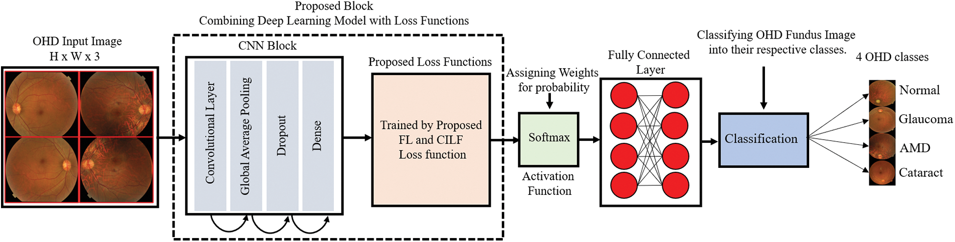
Figure 1: Proposed model architecture

3.1.1 Backbone CNN

To extract features, the proposed model has developed a straightforward CNN network. CNN, in its most basic form, is composed of three distinct layers, which are the convolutional layer (ConvL), the global average pooling layer (GAPL), and the fully connected layer (FCL). RFCI of size 299 × 299 × 3 are input into the CNN model so that the suggested model may be trained on them. The number of channels (Cn) in the input image is three in this case. The ConvL is the first one to be processed. This layer uses filters of the size (IH, IW), where IH (= 3) represents the filter height, and IW (= 3) represents the filter width. Filters are also sometimes referred to as “kernels”. The filter height (IH) and width (IW) will often not change from their default settings. In certain contexts, this filter may also be referred to as the “feature identifier.” The layer can acquire low-level properties such as edges and curves as a result of using these filters. The more ConvL that are included in the model, the better it can extract deep information from RFCI; as a result, the model can recognize all visual characteristics. The model has been incrementally improved by the addition of more ConvL. Convolution is performed on a portion of the image that is selected by the filter. Utilizing the image’s filter and the values of its pixels, the convolution approach requires element-by-element multiplication and adding up the results. These values are referred to as weights or parameters, depending on the context. The model has to go through training to learn these weights. This area of the image is referred to as the “receptive field,” and it plays an important role. The convolution process starts at the very beginning of the RFCI image when the filter is applied. Convolution is then repeatedly carried out as it is continuously moved across the whole image by a predetermined number of units. This process continues until the entire image has been covered. A single operation will only ever provide a single result. The results of applying convolution on the whole image are either an array or a measure of the values. The operation may be written out as indicated in Eqs. (1) and (2).

C=R ×H(1)

C=∑∑R ×( a+i, b+j) ×H (IH, IW)(2)

where R represents the input RFCI image and H represents the filter with the size (IH, IW), respectively. The operator, which is denoted by the symbol (×) stands for the operation. Another parameter that defines the amount that the filter is shifted from its original position is called stride. In the model, each convolutional layer has its stride parameter set to 1, which is the default value. As the number of strides rises, the height and width of the input volume begin to diminish. If the stride number for the minimum overlap of the receptive field is too high, there is a possibility that there may be problems. These problems may include the receptive field being larger than the input volume or the dimensions being smaller.

Padding is used so that these concerns may be addressed. The term “zero padding,” which is synonymous with the term “same padding,” refers to the practice of padding the input with zero while ensuring that the output volume dimension remains the same as the input volume dimension. In this investigation, the value of stride was initially set to 1, and then Eq. (3) was applied to determine the size of the zero padding.

Zero Padding=S−12(3)

where S denotes either the height or the width of the filter; in this instance, both dimensions are the same. Because the proposed model made use of “valid padding” rather than zero padding, the output dimension did not match the size of the input dimension, and it became smaller as a result of the convolution process. To extract a wide variety of characteristics, the convolutional layer made extensive use of a wide variety of filters. There were 32 different filters used in the first layer. For progression, the number of filters increased from 32 to 128, then from 128 to 512, and so on. Furthermore, the activation map refers to the volume output. Eqs. (4)–(6) are used to calculate the output volume.

VH=IH−SH+(2×Z)T+1(4)

VW=IW−SW+(2×Z)T+1(5)

Vn=Ns(6)

where IH represents the height of the input, IW represents the width of the input, SH represents the height of the filter, SW represents the width of the filter, T is the size of the stride, Z represents the padding, and NS represents the number of filters. Regarding the first layer of convolutional processing.

After the convolution step, a nonlinear activation is performed on the result. A linear computation (element-wise multiplication and summation) has been carried out by ConvL. The linear action receives a touch of nonlinearity as a result of this activation. The activation of the convolution output is done via ReLU, which stands for “rectified linear unit”. Eq. (7) is used to calculate the ReLU.

ReLU (Z)=max (0, Z)(7)

In this case, the result of the convolution technique is denoted by Z. Every negative output is brought down to zero by ReLU. The use of ReLU in the model that has been presented is driven by the fact that it enhances the model’s nonlinearity and decreases the amount of time that is spent calculating without affecting the correctness of the model. When training lower layers slowly, also helps mitigate the problem of gradients vanishing altogether. The GAPL is utilized after the two ConvL have been processed. The spatial dimensions of the input are made smaller by this layer. According to the model that has been proposed, the layer is made up of a 2 × 2 filter that has a stride of 2. The filter creates a spiral around the input volume, which results in the highest possible value for the receptive field. The key insight for effectively using this layer is that the feature’s position relative to other features is more significant than the feature’s absolute position. It prevents overfitting and minimizes the number of weights, hence lowering the amount of computing effort that is required. The dropout layer is then used after that. This layer completely gets rid of random activation by setting all of them to zero. Although some activations have been removed, this layer ensures that the model is still able to accurately predict the class label of an RFCI. As a result, it is important to avoid making the model too dependent on the training data. Because of the dropout layer, excessive fitting is avoided. The dropout layers have been added with a threshold of 0.25. A two-dimensional feature map is converted into a one-dimensional feature vector via the flattened layer, which is subsequently passed on to an FCL.

3.1.2 Loss Functions

The loss function is used to evaluate the difference between the expected value and the actual value; hence, the network in the DL model works toward decreasing the predicted loss to achieve optimal performance. Combining FL [30] with correntropy-induced loss functions (CILF) [31], we present a novel concoction loss function in this study. The purpose of this function is to successfully treat difficult biological datasets that contain class imbalance and outliers. The cross-entropy of the binary bits will result in a change to the focal loss. Eqs. (8) and (9) present the definition of binary cross entropy.

Fbce(A^, A)=−AlogA^−(1−A)log(1−A^)(8)

Fbce(A^, A)={−logA^,A=1−log (1−A^),otherwise (9)

D={A,^A=11− A^,Otherwise(10)

Eq. (11) is used to measure the cross entropy method.

Fbce(D)=−log (D)(11)

The FL function, which is based on cross-entropy, adds a modulating factor (1-D)P to decrease the weight of easy examples and direct the training’s focus on more challenging cases. Eq. (12) is used to measure the FL based on cross-entropy.

F(D)=−(1−D)Plog (D)(12)

where a focusing parameter is denoted by P. The contribution of simple samples will decrease as the amount of the concentrating parameter is increased. To further address the issue of class imbalance, the concept of focus loss has been integrated with a weighting element denoted by the symbol W. The FL is further redefined in Eq. (13).

F(D)=− W (1−D)Plog (D)(13)

In addition, by providing a specification for the variable D, the FL may alternatively be expressed as (see Eq. (14)):

F (A^, A)={− W (1−A^)P Log A^,A=1− (1−W)A^Plog (1− A^),otherwise(14)

The advantage of using CILF for classification is that it is adaptable to sample distances via the use of a variety of F norm adjustments. This allows it to be resistant to noise and outliers [32,34]. The F1 norm for relatively slight mistakes is possessed by CILF, which has this quality. CILF behaves in a manner that is analogous to the F2 norm when the error value is small but eventually reaches the F3 norm when the error value is sufficiently large. Eqs. (15) and (16) is used to measure CILF.

C(A, B)=E [M (A−B)](15)

C(A, B)=∫M (a−b) d GAB (a, b)(16)

Fg(A^,A)=1−M (A− A^)(17)

In this case, the Gaussian kernel is used to compute the CILF. Eq. (17) is further modified (see Eqs. (18) and (19)).

Fg(A^,A)=1−Gaussian (A− A^)(18)

Fg(A^,A)=1−exp⁡(−(A−A^)2σ2)(19)

In addition, the CILF may improve model performance without causing an increase in the expenses associated with computation. As a consequence of this, the computing cost of CILF and cross-entropy loss are the same when using a Gaussian kernel.

3.1.3 Concoction of Loss Functions

For this study, by combining the FL and CILF loss functions, we suggest a combining loss function that we refer to as the FL-CILF and its definition is as follows (see Eq. (20)):

HFL+CILF={FD(A^,A), 0 <e≤t Fg(A^,A), t <e<E(20)

where e represents the current epoch and t refers to a previously established cutoff point. We begin the training with focused loss and continue with t epochs of that before switching to Fg loss to finish out the training. The total number of epochs is denoted by the letter E in this context.

The CILF has several advantages, including better generality and noise robustness; but, since it is nonconvex, it may lead to local minima in certain cases. These minima might be problematic. As a result, we use FL to pre-train the model over a large number of epochs. The FL is used to remedy the problem of class imbalance as well as to increase the weight of hard samples.

3.2 Performance Metrics

Several different evaluation metrics, such as recall (REC), specificity (SPF), F1-measure, accuracy (ACU), kappa score (KS), the area under the receiver operating curve (AUC), and the average (AVG), are used to evaluate the classification performance of the suggested model. There is an inverse link between REC and SPF [4], which means that when REC increases, SPF tends to decrease, and vice versa. High REC tests will offer positive findings for those who have an illness, whereas high SPF tests will show that patients with negative results do not have a problem [6]. High REC tests will provide positive results for persons who have an illness. These metrics are measured using Eqs. (21)–(31) that are shown below.

REC=TPTP+FN(21)

SPF=TNTN+FP(22)

ACU=TP+TNTP+TN+FP+FN(23)

F1−measure=2TP2TP+FN+FP(24)

KS=So−Se1− Se(25)

So=∑h=1hTPh∑h=1h(TPh+FNh)(26)

Se=∑h=1 hTPh∗ (TPh+FNh)N2(27)

TPR=TPTP+FN(28)

FPR=FPFP+TN(29)

AUC=∫a=01TPR (FPR−1(a))dx(30)

AVG=1(KS)+(F1−measure)+(AUC)(31)

where the symbols TP and TN stand, respectively, for the true positive and the true negative. The number of samples that were put through the testing procedure is denoted by the letter N. In addition, the value of a false positive is represented by the symbol FP, whereas the value of a false negative is shown by the symbol FN.

4  Results and Discussions

This section presents the experimental results that were obtained from the two publicly accessible OHD datasets. These findings are presented in the context of a comparison between the proposed model and several baseline models, including DenseNet-169, EfficientNet-B7, ResNet-101, Inception-V3, and VGG-19. In addition, the ablation investigation that is associated with the suggested model is carried out in this part.

4.1 Dataset Description and Data Augmentation

For this study, we used two publically available benchmark RFCI datasets [31,32] for training and evaluating the proposed model. The first dataset [31] contains a total of 601 RFCI images including 300 images of the normal category, 101 images of CATR, 100 fundus images of GLU, and 100 images of AMD. The second dataset is from the 2019 University International Competition and is called Ocular Disease Intelligent Recognition (ODIR-2019). The dataset consists of a variety of OHD, such as normal, GLU, CATR, and AMD groups. Both the RFCI and additional information, such as the patient’s age, are considered and used when building the labels that are applied at the patient level. There are a total of 5000 examples included with the first release of the RCFI; however, only 4020 of those specific cases have been reviewed, discussed, and made accessible to the general public. The sample RFCI images from both of the datasets are depicted in Fig. 2.

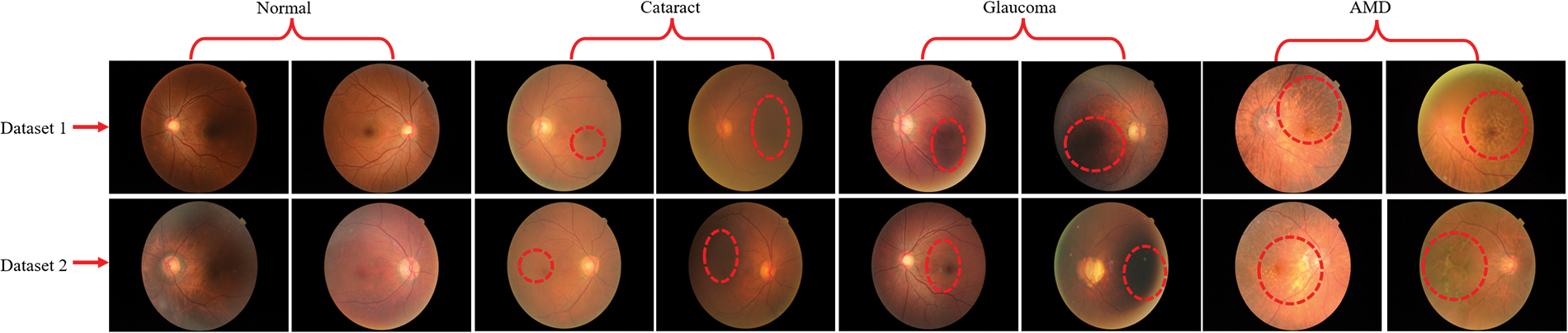
Figure 2: RFCI images of OHD collected from two different datasets. Additionally, the red dotted line represents the infected region of the eyes

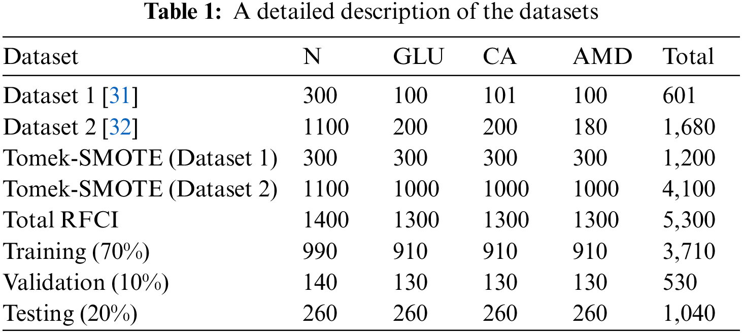
After the strategy has been put into action, we analyze the data from the RFCI using these photographs to determine how successful the strategy was. In the process of cross-validation, training is carried out on each combination of the first two folds, and testing is carried out on the third fold. This is done due to the very little amount of data that is available. This motivates the employment of the Tomek-SMOTE method for expanding the RFCI dataset. Tomek-SMOTE is applied to studies of underrepresented groups like GLU, CATR, and AMD. The whole of the dataset, both with and without the use of Tomek-SMOTE methods, is shown in Table 1. There are 5,300 examples total, and they have been arbitrarily split up into three groups: 530 for validation, 3,710 for training, and 1,060 for assessment. At last, we provide an average of the findings obtained from three different cross-validation tests performed on the test folds.

4.2 Experimental Setup

The CNNs used in the system are the primary focus of this investigation on the effect that different suggested models and various baseline models of variable depths have on the process of feature extraction. When working with CNNs, it is necessary to use the approach of initializing the backbone that has already been trained on ImageNet. As a result of the fact that the data that was utilized to construct the RFCI picture originated from a wide variety of hospitals and sources, it has a diversity of resolutions. This is because the information was collected using several various kinds of technology. Initially, the resolution of each RFCI is reduced to 299 by 299 pixels by scaling them down. As a component of the picture enhancement process that takes place during the training of a network, the random cropping of photo patches measuring 199 by 199 pixels is carried out. During the testing phase, we will employ the complementary strategy of central cropping. Keras was utilized to implement both the proposed model and the baseline models. Python is used for the programming of methods that are not directly connected to convolutional networks. The experiment was conducted using a personal computer that used the Windows operating system and had an 11 GB NVIDIA GPU in addition to 32 GB of RAM for data storage.

4.3 Models Configuration

Different hyperparameters have been used to fine-tune the proposed model. The most significant tool for training CNN with the multi-label classification loss function that is defined by Eqs. (8)–(20) is the stochastic gradient descent (SGD) optimizer. In addition, the batch size is predetermined to be 16, and the initial learning parameter is predetermined to be 0.0001, although it will gradually decrease as the training moves on. Both the dropout rate and the input size are set to 0.2, and the size of the input is 299 by 299. For each experiment, a total of one hundred epochs are carried out, however, we only keep the data from the very last epoch.

4.4 Ophthalmic Disease Classification Using Proposed and Baseline Models

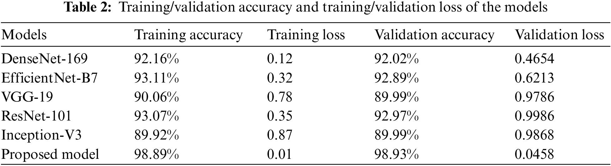
The results of the training and validation are presented in Table 2, which breaks down the results by epoch. The three baseline models, and the proposed CNN model, were run for as many as 100 iterations. The highest level of accuracy that could be attained via training was 98.89%, while the highest level that could be reached through validation was 98.93%. These results suggested that the model learned well and was able to accurately classify GLU, CATR, and AMD in comparison to the normal distribution. The loss during training was 0.0011, whereas the loss during validation was 0.0458.

The suggested CNN has the authority to carry out the procedure of independently getting characteristics from RFCI. DenseNet-169, EfficientNet-B7, ResNet-101, Inception-V3, and VGG-19 with variable depths have the potential to extract features from the data with increasing degrees of abstraction using the aforementioned models. The characteristics that are produced by the model that is being proposed. CNN is swiftly fused by making use of FL and CILF, even though an explicit fusion strategy has not been described. Table 3 provides detailed results of classifying OHD using RFCI.

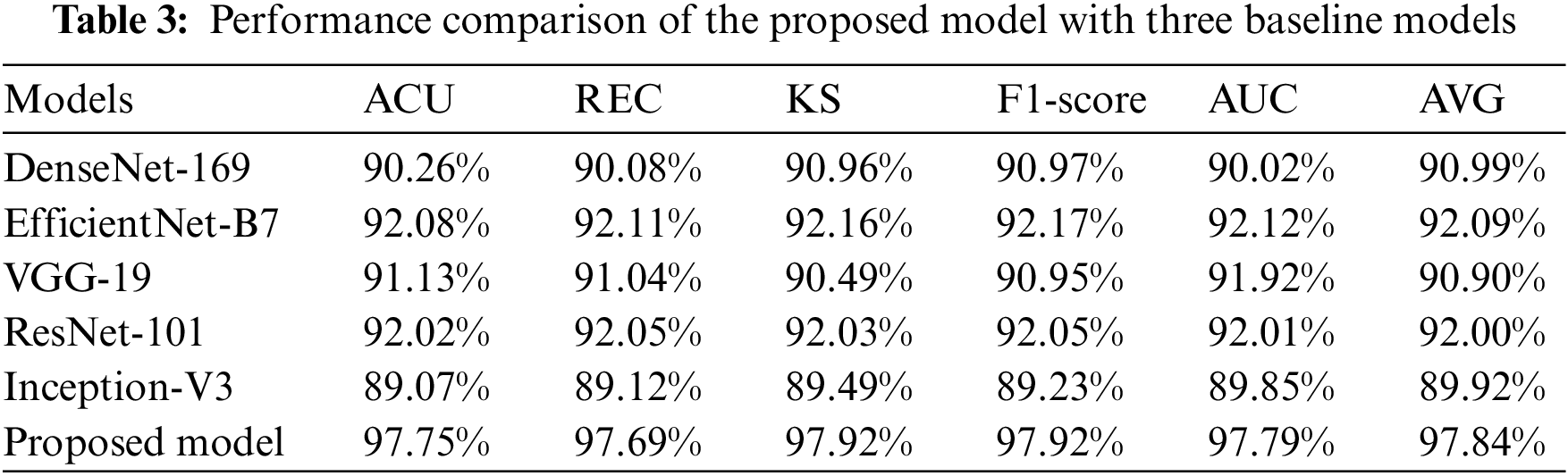
As evidenced by the results, the suggested model outperforms the three baseline models. A score of 97.75% is obtained for the ACU, 97.69% is obtained for the REC, 97.92% is obtained for the KS, and 97.92% is obtained for the F1-score. EfficientNet-B7 achieves a considerable performance improvement in contrast to the baseline models, and it also obtains a classification accuracy of 92.08%. We find that the results of the proposed models improve upon those of DenseNet-169, EfficientNet-B7, ResNet-101, Inception-V3, and VGG-19 by a mean of 6.8% (for the ACU), 4.4% (for the REC), 5.9% (for the F1-score), 6.2% (for the KS), and 8.68% (for the final AVG). This is evidence that the OHD has increased its ability to differentiate between different levels of abstraction in the data it collects. It has been demonstrated that models that employ FL and CILF eventually arrive at a performance plateau. Studies [21,27] that are analogous to the one that is being discussed here have demonstrated that the performance of a network cannot climb linearly with the number of connections that are made between the nodes that are contained within the network. The following are three conclusions that could explain this phenomenon. The fact that the gradient is invisible when viewed from certain perspectives is the first challenge. When one has access to a higher quantity of data, the process of improving a network becomes more complex for optimizing [15]. A decrease in the reuse of such features is the second factor that leads to the inefficient use of the vast number of features created for deep networks [16]. This factor is responsible for the inefficiency that results from the usage of those features. Since there are only a certain number of training samples that can be obtained, the network has not yet been completely trained to its full potential.

During the training procedure for the proposed model and three different baseline CNN classifiers, the obtained features were utilized throughout the entire process. The grid search approach was utilized so that the ideal values could be determined for the hyperparameters. When it comes to the process of training the models that are being utilized, the method of 5-fold cross-validation is the one that is used. To verify the accuracy of the model, several diverse performance criteria were applied to the challenge of differentiating between the various OHD types. The confusion matrices for the proposed model, DenseNet-169, EfficientNet-B7, ResNet-101, Inception-V3, and VGG-19 are shown in Fig. 3. The model that was given was successful in recognizing 255 out of 260 instances of OHD, even though it misclassified two cases as AMD, two cases as CATR, and one case as GLU. In the example of DenseNet-169, in which extracted attributes were utilized to train the model, the model accurately recognized 238 cases of AMD disease out of a total of 260 cases, however, it mistakenly labeled 22 cases as normal and as having other OHD disorders such as CATR and GLU. There were 243 cases of CATR sickness, and EfficientNet-B7 correctly predicted the class label for each one of them. On the other hand, 17 of the cases were wrongly classified as normal, AMD, or GLU. In total, 243 out of 260 GLU disease cases had a class label that was accurately predicted by VGG-19. On the other hand, it mistakenly classified five patients as normal, five as AMD, and seven as CATR.

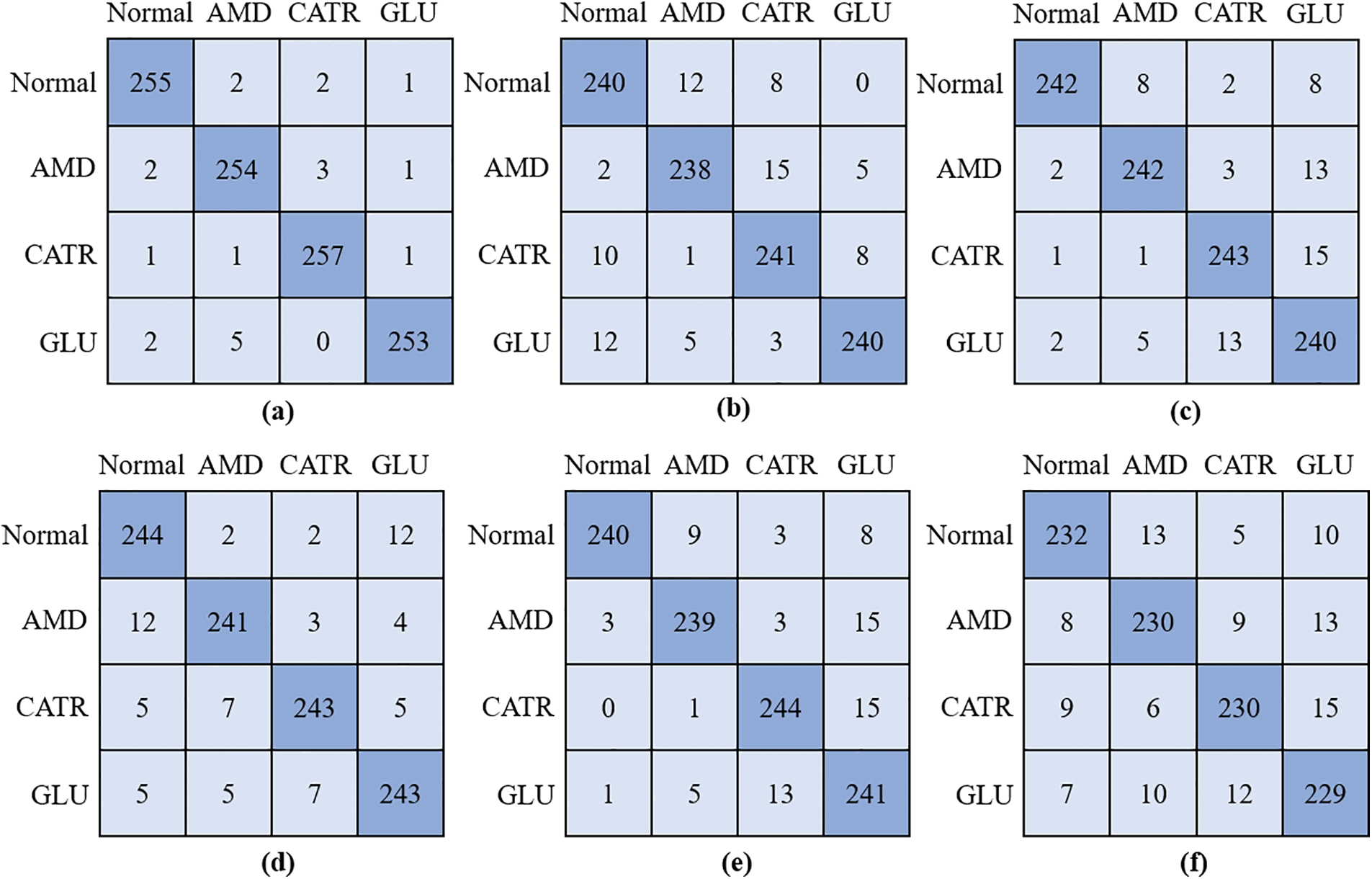
Figure 3: Confusion matrix; (a) proposed model, (b) DenseNet-169, (c) EfficientNet-B7, (d) VGG-19, (e) ResNet-101, and (f) Inception-V3

4.5 Proposed Model Computational Complexities

An in-depth study of the properties of the network can be found in Table 4, along with information on the level of complexity the network possesses and the number of floating-point operations done per second (FLOPS). Because of this, we are in a position to evaluate the results of the classification in a manner that is not only just but also objective.

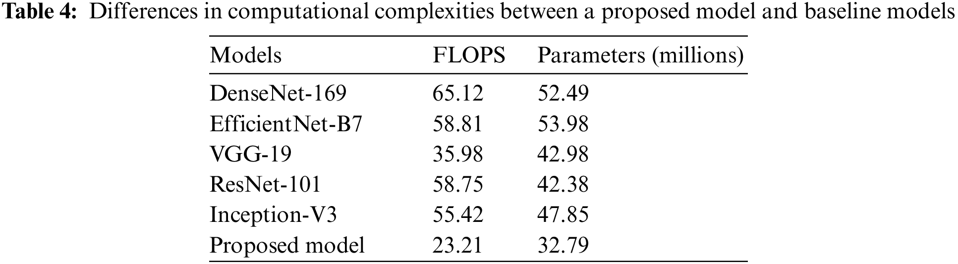
The proposed approach may still be significantly more innovative than the baseline, even when FLOPs or network considerations are used. While employing fewer FLOPs than the DenseNet-169, EfficientNet-B7, ResNet-101, Inception-V3, and VGG-19 baselines, networks that employ the proposed CNN with FL and CILF get better results. This shows that the increasing complexity of the underlying networks is not the only explanation for the method’s impressively precise classification results. We can improve OHD patient-by-patient diagnosis using RFCI. If improved classification performance is desired, it is crucial to make use of the data provided by RFCI. Specifically, the importance of the diagnosis at the patient level [29]. Implementing FL and CILF will very probably result in a significant rise in network parameters, even if the increase in FLOPs is modest.

4.6 Training Time

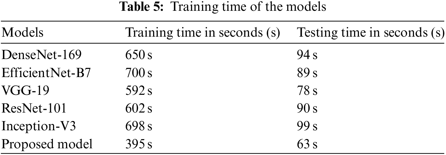
The amount of time required to train the proposed model as well as many existing baseline models is shown in Table 5. According to the findings, the training process for DenseNet-169 on the complete dataset takes 650 seconds (s). It takes 700 s to train the EfficientNet-B7 model, and 592 s to train the VGG-19 model. As compared to existing models, the proposed approach requires much less time to train. This is because the proposed model has fewer trainable parameters than earlier models.

4.7 Ablation Study

During our study, we developed a novel model by making use of both the FL and the CILF. As a consequence of this, more intricate iterations of the CNN model were constructed. To determine whether or not the suggested model applies to all three OHD, including the normal condition, we conducted a statistical analysis of the experimental data while simultaneously controlling a variable. Throughout the experiment, the ACU and KS values of each model were analyzed and compared with the assistance of metrics to establish the degree to which the upgraded module contributed to the overall importance of the model. The fundamental CNN model is explained in Experiment 1, potential implementation in FL is shown in Experiment 2, and the proposed model is compared to FL and CILF in Experiment 3. Table 6 provides tabular data illustrating the experiment’s findings.

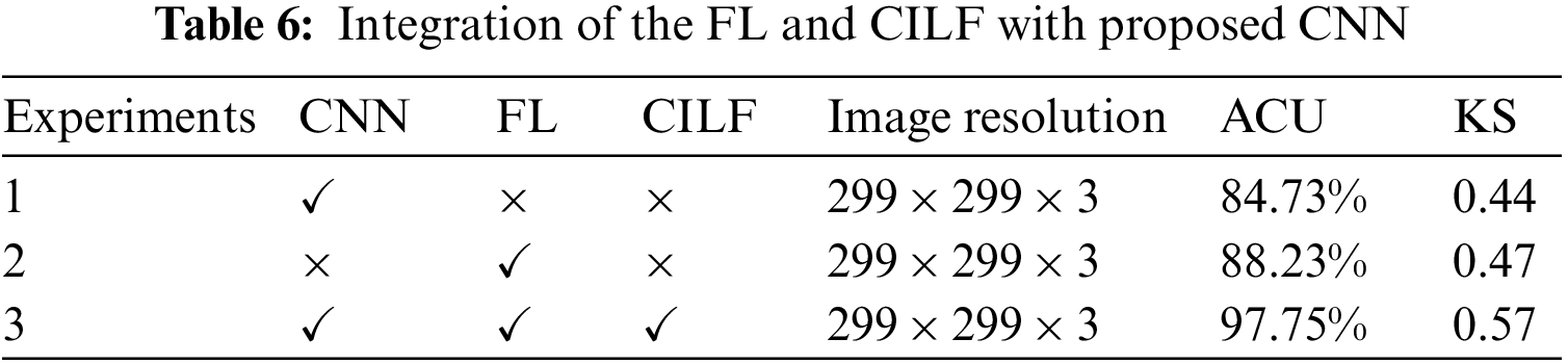
When the findings of Experiment 1 are compared to those of Experiment 2, it is clear that the modifications that we propose lead to an improvement of 3.5% in the model’s overall accuracy of OHD categorization. During Experiment 3, we combined the FL and CILF with CNN, which resulted in the development of the suggested model. In comparison to Experiment 2, the suggested model increased by 9.52 percentage points in OHD categorization.

4.8 Comparison with State-of-the-Arts

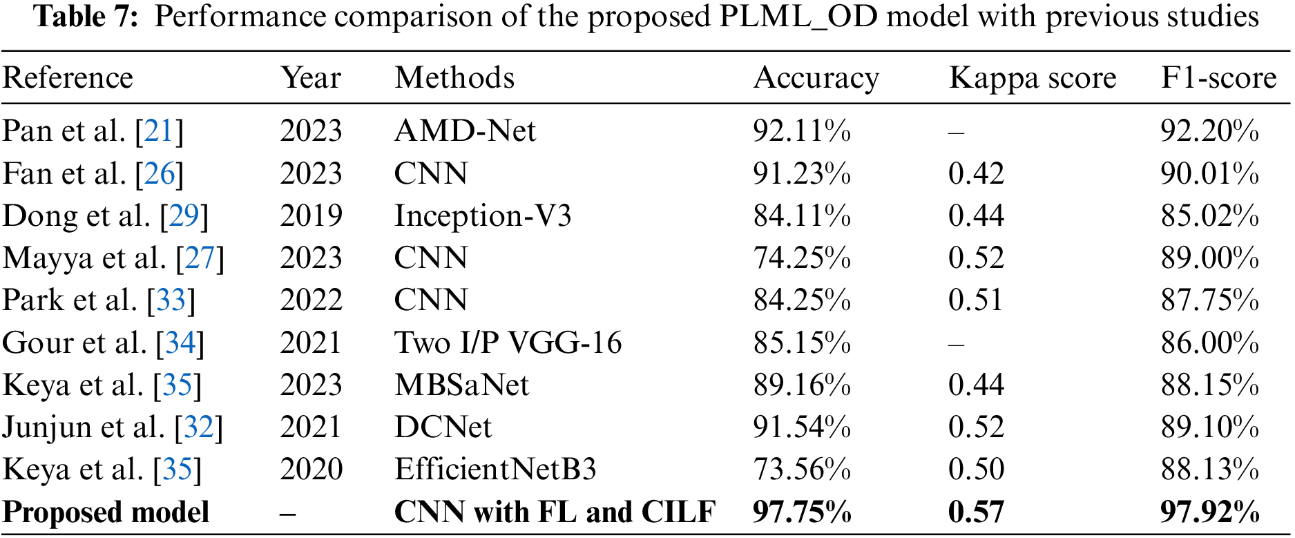
In this section, we compare the performance of the proposed model to that of contemporary state-of-the-art (SOTA) classifiers on several different criteria. These characteristics include accuracy, kappa score, and F1-score, among many others. The novel Inception-V3 model created by Junayed et al. [31] achieved an accuracy of 0.84 in OHD categorization. The majority of these researches [32,34] used color fundus pictures to classify GLU using a CNN model. The accuracy, kappa, and F1 scores for classifying GLU and CATR using the CNN model used in the study [33] were 91.0%, 0.42, and 0.90, respectively. Keya et al. [35] introduced a new model they called MBSaNet, which had a precision of 0.89. Table 7 presents a comprehensive examination of the suggested model of the prior literature.

4.9 GRAD-CAM of OHD Using Proposed Model

To offer a graphical representation of the data that were produced by the suggested model, we made use of the Grad-CAM heatmap technique. The major goal of the heatmap is to attract attention to the key component of the RFCI that the model concentrates on highlighting. Fig. 4 provides a visual example of the heatmap that may be generated by using the suggested approach.

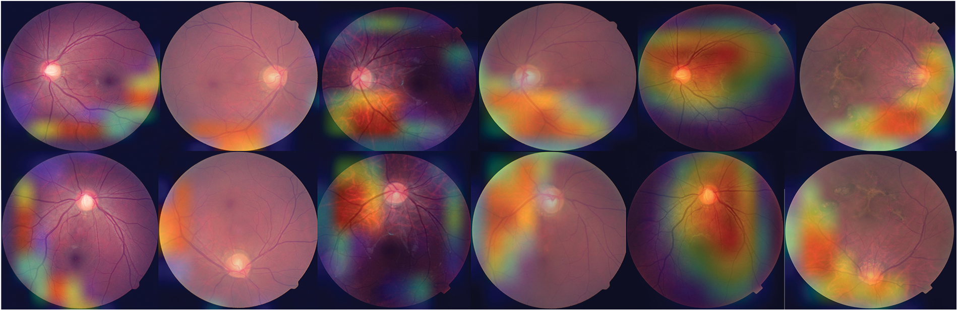
Figure 4: Heat map of three OHD diseases developed using the proposed model

4.10 Discussions

DL techniques have been applied to assist in the diagnosis of the three most common causes of blindness, which are AMD, CATR, and GLU. For this study, we designed a novel DL model with the concoction of FL and CILF to classify the OHD disease. The purpose of adding these two loss functions is to handle the class imbalance and the problem of outliers in the complicated OHD datasets. The proposed model is trained on two publically available benchmarks RFCI datasets [31,32] using fundus images. In addition, the results of the proposed model are contrasted with those of the baseline models and with the current state of the classifiers. The proposed model outperforms the five baseline models and achieved 97.75% accuracy with a 0.57 kappa score. Additionally, the proposed model can handle the imbalance class problem by using SMOTE-Tomek. The proposed model is well suited for classifying three common OHD diseases such as CATR, AMD, and GLU. However, the limitation of this study is that the proposed model is not suited for other OHD diseases such as amblyopia, strabismus, and refractive errors.

5  Conclusion

By the examination of RFCI, this study puts up the idea of a DL-based CAD model as a solution to a difficult problem in the categorization of OHD images. We provide a technique for the identification of OHD that is based on DL and is comprised of a CNN combined with the proposed FL and CILF functions. Meanwhile, Tomek-SMOTE was used to handle the imbalance class problem. The suggested model’s effectiveness in terms of classification was assessed using two datasets that were made accessible to the public, each of which included four distinct OHD. When it came to categorizing OHD, the suggested model was able to attain a classification accuracy of 97.75%. The results reveal that the proposed method achieves superior results in terms of classification accuracy, sensitivity, specificity, Kappa, and AUC in experiments when compared to other standard DL-based classifiers. This is mostly because of the inclusion of a mixed loss function in the algorithm. The findings of the studies provide evidence that the DL strategy that we suggested is both successful and resilient when used in the categorization of ocular disorders. A federated learning-based collaborative model will be developed in the future with the participation of several medical facilities, and it will be done so with full regard for the privacy of individual patients’ medical records.

Acknowledgement: Our deepest thanks to the Deanship of Scientific Research at King Faisal University, Alhofuf, KSA, for their support to conduct this research.

Funding Statement: This work was supported by the Deanship of Scientific Research, Vice Presidency for Graduate Studies and Scientific Research, King Faisal University, Saudi Arabia [Grant No. 3,363].

Author Contributions: Study conception and design: Ali Haider Khan, Sayyid Kamran Hussain; data collection: Ali Haider Khan, Sayyid Kamran Hussain, Sajid Iqbal; analysis and interpretation of results: Ali Haider Khan, Sayyid Kamran Hussain, Sajid Iqbal; draft manuscript preparation: Malek Alrashidi, Qazi Mudassar Ilyas and Kamran Shah; supervision: Ali Haider Khan, Sajid Iqbal. All authors reviewed the results and approved the final version of the manuscript.

Availability of Data and Materials: The authors declare that all data supporting the findings of this study are available within the article and publicly accessible.

Conflicts of Interest: The authors declare that they have no conflicts of interest to report regarding the present study.

References

1. P. Charry, O. Julián and F. A. González, “A systematic review of deep learning methods applied to ocular images,” Ciencia e Ingeniería Neogranadina, vol. 30, no. 1, pp. 9–26, 2022. [Google Scholar]

2. W. Xiao, H. Xi, H. W. Jing, R. L. Duo, Z. Yi et al., “Screening and identifying hepatobiliary diseases through deep learning using ocular images: A prospective, multicentre study,” The Lancet Digital Health, vol. 3, no. 2, pp. e88–e97, 2021. [Google Scholar] [PubMed]

3. W. Zhenhua, Y. Zhong, M. Yao, Y. Ma, W. Zhang et al., “Automated segmentation of macular edema for the diagnosis of ocular disease using deep learning method,” Scientific Reports, vol. 11, no. 1, pp. 1–12, 2021. [Google Scholar]

4. G. Parampal, F. Oloumi, U. Rubin and M. T. S. Tennant, “Deep learning in ophthalmology: A review,” Canadian Journal of Ophthalmology, vol. 53, no. 4, pp. 309–313, 2018. [Google Scholar]

5. G. Hao, Y. Guo, L. Gu, A. Wei, S. Xie et al., “Deep learning for identifying corneal diseases from ocular surface slit-lamp photographs,” Scientific Reports, vol. 10, no. 1, pp. 1–11, 2020. [Google Scholar]

6. Z. Kai, X. Liu, F. Liu, L. He, L. Zhang et al., “An interpretable and expandable deep learning diagnostic system for multiple ocular diseases: Qualitative study,” Journal of Medical Internet Research, vol. 20,no. 11, pp. e11144, 2018. [Google Scholar]

7. M. Hassaan, M. S. Farooq, A. Khelifi, A. Abid, J. N. Qureshi et al., “A comparison of transfer learning performance versus health experts in disease diagnosis from medical imaging,” IEEE Access, vol. 8, no. 1, pp. 139367–139386, 2020. [Google Scholar]

8. D. Wang and W. Liejun, “On OCT image classification via deep learning,” IEEE Photonics Journal,vol. 11, no. 5, pp. 1–14, 2019. [Google Scholar]

9. B. Liefers, G. V. Freerk, S. Vivian, V. G. Bram, H. Carel et al., “Automatic detection of the foveal center in optical coherence tomography,” Biomedical Optics Express, vol. 8, no. 11, pp. 5160–5178, 2017. [Google Scholar] [PubMed]

10. T. Nazir, I. Aun, J. Ali, M. Hafiz, H. Dildar et al., “Retinal image analysis for diabetes-based eye disease detection using deep learning,” Applied Sciences, vol. 10, no. 18, pp. 6185, 2020. [Google Scholar]

11. D. S. Q. Ting, R. P. Louis, P. Lily, P. C. John, Y. L. Aaron et al., “Artificial intelligence and deep learning in ophthalmology,” British Journal of Ophthalmology, vol. 103, no. 2, pp. 167–175, 2019. [Google Scholar] [PubMed]

12. O. Ouda, A. M. Eman, A. A. E. Abd and E. Mohammed, “Multiple ocular disease diagnosis using fundus images based on multi-label deep learning classification,” Electronics, vol. 11, no. 13, pp. 1966, 2022. [Google Scholar]

13. T. K. Yoo, Y. C. Joon, K. K. Hong, H. R. Ik and K. K. Jin, “Adopting low-shot deep learning for the detection of conjunctival melanoma using ocular surface images,” Computer Methods and Programs in Biomedicine, vol. 205, pp. 106086, 2021. [Google Scholar] [PubMed]

14. X. J. Meng, X. Xi, L. Yang, G. Zhang, Y. Yin et al., “Fast and effective optic disk localization based on convolutional neural network,” Neurocomputing, vol. 312, pp. 285–295, 2018. [Google Scholar]

15. S. M. Zekavat, K. R. Vineet, T. Mark, Y. Yixuan, K. Satoshi et al., “Deep learning of the retina enables phenome-and genome-wide analyses of the microvasculature,” Circulation, vol. 145, no. 2, pp. 134–150, 2022. [Google Scholar] [PubMed]

16. B. Hassan, Q. Shiyin, H. Taimur, A. Ramsha and W. Naoufel, “Joint segmentation and quantification of chorioretinal biomarkers in optical coherence tomography scans: A deep learning approach,” IEEE Transactions on Instrumentation and Measurement, vol. 70, pp. 1–17, 2021. [Google Scholar]

17. Y. Yahan, R. Li, D. Lin, X. Zhang, W. Li et al., “Automatic identification of myopia based on ocular appearance images using deep learning,” Annals of Translational Medicine, vol. 8, no. 11, pp. 7–22, 2020. [Google Scholar]

18. K. Y. Wu, K. Merve, T. Cristina, J. Belinda, H. N. Bich et al., “An overview of the dry eye disease in sjögren’s syndrome using our current molecular understanding,” International Journal of Molecular Sciences, vol. 24, no. 2, pp. 1580, 2023. [Google Scholar] [PubMed]

19. F. Livia, S. K. Wagner, D. J. Fu, X. Liu, E. Korot et al., “Automated deep learning design for medical image classification by health-care professionals with no coding experience: A feasibility study,” The Lancet Digital Health, vol. 1, no. 5, pp. 232–242, 2019. [Google Scholar]

20. J. Kanno, S. Takuhei, I. Hirokazu, I. Hisashi, Y. Yuji et al., “Deep learning with a dataset created using Kanno Saitama macro, a self-made automatic foveal avascular zone extraction program,” Journal of Clinical Medicine, vol. 12, no. 1, pp. 183, 2023. [Google Scholar]

21. L. Pan, L. Liang, Z. Gao and X. Wang, “AMD-Net: Automatic subretinal fluid and hemorrhage segmentation for wet age-related macular degeneration in ocular fundus images,” Biomedical Signal Processing and Control, vol. 80, pp. 104262, 2023. [Google Scholar]

22. A. H. Khan, H. Malik, W. Khalil, S. K. Hussain, T. Anees et al., “Spatial correlation module for classification of multi-label ocular diseases using color fundus images,” Computers, Materials & Continua, vol. 76, no. 1, pp. 133–150, 2023. [Google Scholar]

23. S. Ahlam, E. M. Senan and H. S. A. Shatnawi, “Automatic classification of colour fundus images for prediction eye disease types based on hybrid features,” Diagnostics, vol. 13, no. 10, pp. 1706, 2023. [Google Scholar]

24. C. C. Yang, D. Y. Hsu and C. H. Chou, “Predicting the onset of diabetes with machine learning methods,” Journal of Personalized Medicine, vol. 13, no. 3, pp. 406, 2023. [Google Scholar]

25. J. Y. Choi, K. Y. Tae, G. S. Jeong, K. Jiyong, T. U. Terry et al., “Multi-categorical deep learning neural network to classify retinal images: A pilot study employing small database,” PLoS One, vol. 12, no. 11,pp. e0187336, 2017. [Google Scholar] [PubMed]

26. R. Fan, A. Kamran, B. Christopher, C. Mark, B. Nicole et al., “Detecting glaucoma from fundus photographs using deep learning without convolutions: Transformer for improved generalization,” Ophthalmology Science, vol. 3, no. 1, pp. 100233, 2023. [Google Scholar] [PubMed]

27. V. Mayya, K. Uma, K. S. Divyalakshmi and U. A. Rajendra, “An empirical study of preprocessing techniques with convolutional neural networks for accurate detection of chronic ocular diseases using fundus images,” Applied Intelligence, vol. 53, no. 2, pp. 1548–1566, 2023. [Google Scholar] [PubMed]

28. N. M. Dipu, A. S. Sifatul and K. Salam, “Ocular disease detection using advanced neural network based classification algorithms,” Asian Journal for Convergence in Technology, vol. 7, pp. 91–99, 2021. [Google Scholar]

29. W. Dong, N. Pu, S. Li, Y. Wang and Y. Tao, “Application of iontophoresis in ophthalmic practice: An innovative strategy to deliver drugs into the eye,” Drug Delivery, vol. 30, no. 1, pp. 2165736, 2023. [Google Scholar]

30. W. Jing, L. Yang, Z. Huo, W. He and J. Luo, “Multi-label classification of fundus images with EfficientNet,” IEEE Access, vol. 8, pp. 212499–212508, 2020. [Google Scholar]

31. M. S. Junayed, M. B. Islam, S. Arezoo and R. Saimunur, “CataractNet: An automated cataract detection system using deep learning for fundus images,” IEEE Access, vol. 9, pp. 128799–128808, 2021. [Google Scholar]

32. H. Junjun, C. Li, J. Ye, Y. Qiao and L. Gu, “Multi-label ocular disease classification with a dense correlation deep neural network,” Biomedical Signal Processing and Control, vol. 63, pp. 102167, 2021. [Google Scholar]

33. K. B. Park and Y. L. Jae, “SwinE-Net: Hybrid deep learning approach to novel polyp segmentation using convolutional neural network and swin transformer,” Journal of Computational Design and Engineering, vol. 9, no. 2, pp. 616–632, 2022. [Google Scholar]

34. N. Gour and K. Pritee, “Multi-class multi-label ophthalmological disease detection using transfer learning based convolutional neural network,” Biomedical Signal Processing and Control, vol. 66, pp. 102329, 2021. [Google Scholar]

35. W. Keya, C. Xu, G. Li, Y. Zhang, Y. Zheng et al., “Combining convolutional neural networks and self-attention for fundus diseases identification,” Scientific Reports, vol. 13, no. 1, pp. 1–15, 2023. [Google Scholar]