
 Submit a Paper
 Propose a Special lssue
 Open Access
ARTICLE

3D Kronecker Convolutional Feature Pyramid for Brain Tumor Semantic Segmentation in MR Imaging
1
Medical Imaging and Diagnostics Lab, NCAI, Department of Computer Science, COMSATS University Islamabad, Islamabad,
44000, Pakistan
2
Department of Electrical and Computer Engineering, COMSATS University Islamabad, Wah Campus, Wah, Pakistan
3
Department of Computer Science, HITEC University, Taxila, Pakistan
4
Department of Management Information Systems, College of Business Administration, Prince Sattam Bin Abdulaziz University,
Al-Kharj, 16273, Saudi Arabia
5
Department of Computer Science, Hanyang University, Seoul, 04763, Korea
* Corresponding Author: Jae-Hyuk Cha. Email:
Computers, Materials & Continua 2023, 76(3), 2861-2877. https://doi.org/10.32604/cmc.2023.039181
Received 13 January 2023; Accepted 10 April 2023; Issue published 08 October 2023
 View Full Text
 Download PDF
Abstract
Brain tumor significantly impacts the quality of life and changes everything for a patient and their loved ones. Diagnosing a brain tumor usually begins with magnetic resonance imaging (MRI). The manual brain tumor diagnosis from the MRO images always requires an expert radiologist. However, this process is time-consuming and costly. Therefore, a computerized technique is required for brain tumor detection in MRI images. Using the MRI, a novel mechanism of the three-dimensional (3D) Kronecker convolution feature pyramid (KCFP) is used to segment brain tumors, resolving the pixel loss and weak processing of multi-scale lesions. A single dilation rate was replaced with the 3D Kronecker convolution, while local feature learning was performed using the 3D Feature Selection (3DFSC). A 3D KCFP was added at the end of 3DFSC to resolve weak processing of multi-scale lesions, yielding efficient segmentation of brain tumors of different sizes. A 3D connected component analysis with a global threshold was used as a post-processing technique. The standard Multimodal Brain Tumor Segmentation 2020 dataset was used for model validation. Our 3D KCFP model performed exceptionally well compared to other benchmark schemes with a dice similarity coefficient of 0.90, 0.80, and 0.84 for the whole tumor, enhancing tumor, and tumor core, respectively. Overall, the proposed model was efficient in brain tumor segmentation, which may facilitate medical practitioners for an appropriate diagnosis for future treatment planning.Keywords
A tumor is a human’s uncontrollable growth of cancer cells [1]. A tumor that grows inside the brain and spreads to nearby locations constitutes the primary tumor. By contrast, a secondary brain tumor has more than one point of origin and then reaches the brain via the process known as brain metastasis [2]. Meanwhile, a glioma is a brain tumor originating from surrounding infiltrating nerve tissues and glial cells [3]. Like other cancers, brain tumors comprise two types: benign and malignant. They are divisible into four grades, i.e., I, II, III, and IV (World Health Organization, year 2000). Grades I and II brain tumors are low-grade benign gliomas, while grades III and IV are high-grade gliomas. Benign brain tumors include meningioma and glioma, while malignant ones are astrocytoma and glioblastoma. Grade IV tumors are the most hazardous tumor; histopathology is a primary method that can be used to classify grade IV tumors from other ones [4].
Based on the attributes of the intra-tumoral regions, brain tumors can be separated into four groups, i.e., edema, non-enhancing nucleus, necrotic and active nucleus [5]. The groups mentioned above derived three classes which further make the segmentation map. The first class is the whole tumor that comprises all four tumor groups. The second class is the core tumor which encompasses all tumor groups except for the edema, and the third class is the enhancing tumor which consists of just the enhancing core [6].
With the technological advancement of medical imaging, modalities are crucial for curing brain tumors. Imaging modalities such as positron emission tomography, ultrasonography, and Magnetic Resonance Imaging (MRI) help to understand many aspects of a brain tumor [4]. In MRI, soft tissues are contrasted to provide vital information about different parameters of brain tumors with nearly no harmful effects of high radiation on humans [7]. MRI scans for diagnosing tumor regions are produced in three anatomical views: coronal, sagittal, and axial [8], segmenting gliomas and other tumor structures for more efficient treatment planning. However, the intensity of MRI images is not homogeneous [9], and scanner are costly [10]. Also, manual segmentation is time-consuming. Consequently, physicians often use rough measures and are prone to errors [11]. Automatic segmentation also encounters challenges with different sizes, shapes, and dimensions of abnormal brain tumors [12].
Meanwhile, Convolutional Neural Network (CNN) is widely used to automatically segment brain tumors, extracting more relevant and accurate features by enhancing the receptive field. However, CNN is computationally intensive, requiring a large kernel size [13]. Different CNN architectures were proposed to resolve the complexity of high computational costs [14]. Other techniques were also used to reduce the filter parameters to improve network performance. For example, Atrous convolution is used to enlarge the receptive field while maintaining a similar resolution for a feature. It captures more contextual information at the same kernel size. Specifically, Atrous filters use zeros to expand vacant positions, preserving the feature size from one layer to another, capturing the global information, and keeping the number of parameters constant [15]. However, due to the increment of the dilation rate, Atrous convolution losses between-pixel information, missing some vital data and yielding inaccurate segmentation [16]. Besides, Deep Convolution Neural Network (DCNN) uses repeated striding convolutional kernels and multiple pooling layers to extract more tissue features [17]. However, it reduces the feature resolutions. In general, most of the existing DCNN techniques have limited capacity for multi-scale processing, hindering the model from improving the performance of brain tumor segmentation. Some deep learning techniques used 3D convolutional networks [18], parallelized long short-term memory (LSTM) [19], and fully connected networks (FCN) [20]. Machine learning-based probabilistic models were merged in many studies to produce a deep-learning model [21], performing automated brain tumor segmentation. Other segmentation methods used the capabilities of 3D-CNN [22] and 2D-CNN [23]. However, 3D-CNN used all 3D information of MRI data, yielding computational complexity due to an increment in the number of parameters. Therefore, 2D-CNN was used for efficient and cost-effective brain tumor segmentation.
Another study [24] proposed a Kronecker approach to resolve the Atrous convolution problem while keeping the number of parameters consistent. Kronecker convolution generates a lightweight model with many trained batches without extensive hardware while increasing the receptive field and implementing the computation of lost features. Also, the discrimination of cancerous and healthy cells becomes possible with contexts around the lesion. The generated feature maps from the three-dimensional (3D) Feature Selection (FSC) block are fed into the multi-input branch pyramid to fuse contexts with lesion features. This ultimately improves model identification for accurate and efficient segmentation without information loss. The key contributions of this study are as follows:
• We have used 3D Kronecker to resolve the loss of pixels in Atrous convolution caused by increased dilation rates.
• The 3D Kronecker Convolution Feature Pyramid (KCFP) model captured multi-scale features of brain tumors.
• Pyramid features are used through the skip connections from the 3D FSC network to overcome the vanishing gradient problem while preserving local features.
• The connected component analysis is combined with a global threshold to reduce false positives for effective structural segmentation.
The rest of this paper is organized as Section 2, literature review. Section 3 gives a detailed overview of our proposed KCFP model. Section 4 presents the Results, and their Discussion Section 5 contains the conclusion.
In 2012, Medical Image Computing and Computer-Assisted Intervention (MACCAI) challenge was introduced. The medical imaging computing and computer-assisted intervention society provided the BraTs dataset to facilitate brain tumor segmentation [25]. Two automated techniques were introduced to segment brain tumors in the past decade. The first was the machine-learning techniques that used various classifications to learn different and diverse features, solving the issue of multi-classes [26]. In addition, these techniques yielded hierarchical segmentations with effective fine scales [27].
Another study [28] used a 2.5D CNN architecture but began with 2D kernels that overlooked inter-size interactions, and hence, crucial contextual information was not captured [29]. Meanwhile, many FCNs prognosticated the predicted segmentation masks effectively [30], but they could not model the context of the label domain [31]. Consequently, a new variant of FCN, that is, U-Net, was developed [32]. Fully connected layers were absent in U-Net. Thus, it would miss the context when identifying the boundary images. The missing contexts were retrieved by merging the images in a mirrored manner. Compared to FCN, U-Net was better because it could capture the skip connections among different pathways.
These skip connections allowed the original image data to repair the details. Also, a modified U-Net was proposed [33], implementing a dice-loss function to resolve overfitting in tumor segmentation. Besides, zero-padding was used to keep the output dimension constant in down and up-sampling paths [34]. Meanwhile, a U-Net with multiple input channels was used for identifying lesions [35]. In the same way, many other approaches are used to improve the segmentation process [36]. Another study proposed a fully connected CNN [37], using low-and high-level feature maps in the final classification.
Similarly, another study [38] developed a V-Net, i.e., a modified 3D U-Net with a dice-loss function, to capture crucial information from the 3D data. Also, a 3D U-Net was developed, using the ground truth of the whole tumor to detect the tumor core. Besides, two U-Nets were used in post-processing to improve the prediction, yielding a better classification of brain tumors [39].
The primary drawback of FCN was that the up-sampling results were unclear, thus decreasing the analytical performance of the medical images. The cascaded architecture was then used to overcome this problem, converting multi-segmentation into binary segmentation [40]. In this respect, two cascades of V-Nets were used to ensure that the training methods concentrated the essential voxels [41]. A multi-class cascaded classifier was also reported [42]. Besides, feature fusion was accomplished using various feature-extraction methods. In general, cascaded networks accounted for the spatial linkages between sub-regions. However, training numerous sub-networks was more complex than just a single end-to-end network. Attention mechanisms were also used to improve brain tumor segmentation [43].
Another study [44] introduced a novel attention gate that targeted structures of various sizes and shapes. Models trained with attention gate suppressed superfluous elements of an input image while emphasizing key features. Also, a 2D U-net-based confined parameter network was developed [45]. It contained an attention learning algorithm to prevent the model from becoming redundant by adaptively weighing each input channel. Besides, a multi-scale network was used to provide enough information to interpret segmentation features [46].
These architectures (machine learning and deep learning) were computationally intensive, requiring a costly hardware setup. Consequently, the segmentation process became highly expensive. Numerous studies were conducted to mitigate the complexity of 3D-CNN.
In particular, the Atrous convolution-based methods were widely used to address this issue. In this respect, a multi-fiber network with Atrous convolution effectively integrated group convolution [47]. It reduced the computational cost of the 3D convolution by merging features at various scales. Besides, weighted Atrous convolutions were used to collect multiple-scale information, reducing inference time and model complexity. Likewise, a multi-scale Atrous convolution was used [48] to sample the high-level refined characteristics of objects. However, Atrous convolution suffers from the loss of information due to missing pixels. Hence, Kronecker convolution was used to mitigate information loss by increasing the receptive field while keeping the same parameters [21]. The related work on medical image segmentation is presented in Table 1.
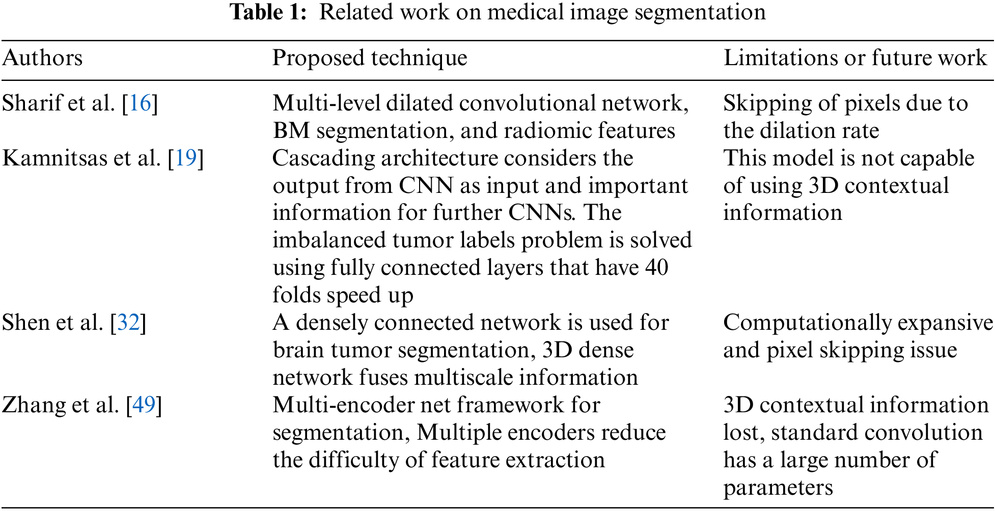
The next section elaborates on the brain tumors segmentation using 3D Kronecker convolution feature pyramid with details of dataset preprocessing, proposed model, post-processing, and performance evaluation metrics.
3 Brain Tumors Segmentation Using 3D Kronecker Convolution Feature Pyramid
This section presents the dataset and pre-processing of the proposed model, performance evaluation, post-processing, and training and model validation.
This study used the standard Multimodal Brain Tumor Segmentation (BraTs) data for brain tumor segmentation. In the BraTs dataset, the primary focus is given to the segmentation of intrinsically heterogeneous (gliomas) by utilizing a dataset of MRI scans from distinct sources. The BraTs 2020 training consisted of 369 volumes, of which 125 were given for validating the dataset. These BraTs datasets comprised MRI scans with four modalities, namely, T1, T2, Flair, and T1-Contrast Enhanced [50]. The dimension of MRI volume dimension is 240 × 240 × 155. The ground truth of the training dataset for each patient was also given. The ground truth contained four classes of segmentation: necrotic, edema, non-tumor, and non-enhancing core. These MRI scans were re-sampled to isotropic voxel resolution at 1 mm^3 as skull stripped. Segmentations were validated on the leaderboard to check the effectiveness of our proposed model. The intensity of the MRI depended on the image acquisition. In this study, variations in intensity and contrast in MRI volume were reduced via normalization, and Z-score [51] was used to normalize the MRI modalities via Eq. (1).
Here, Z describes Z-score, μ represents the mean pixel intensity, and α denotes the standard deviation of the pixel intensity, and X is the pixel value. Normalization wrapped and aligned the image data in the anatomic template for model convergence by attaining the optimal global solution.
Segmentation of the proposed model is comprised of four steps. Firstly, the nibble library was used to load the BraTs multi-modality data, followed by Z-score normalization since deep learning models were sensitive to data diversity. We trained our model simultaneously with all three brain views, i.e., axial, coronal, and sagittal. The data was flipped to coronal, sagittal, and axial planes randomly at the probability of 0.5 to benefit from brain multi-view while augmenting the data to generalize our model. Consequently, when visualizing a slice in a single view (e.g., axial), neighboring pixels in the region of interest could be compared with two other views (sagittal and coronal) [45]. Also, the Gaussian blurring was added to the data to remove noise from MRI images.
Secondly, the model is trained on all three brain views once with brain view augmentation on run time. This pre-processed data, i.e., multi-view data, was then used to train the model. Thirdly, the model was data-validated. Lastly, the validations were post-processed. In this respect, a 3D connected component analysis with a global threshold was used to reduce false positives from model predictions.
This study used a 3D KCFP model to segment brain tumors automatically. The model consisted of three modules: 3D feature selection using a 3DFSC network, multi-scale feature learning using featured pyramids, and post-processing based on 3D connected component analysis with a global threshold. The main flow is shown in Fig. 1.
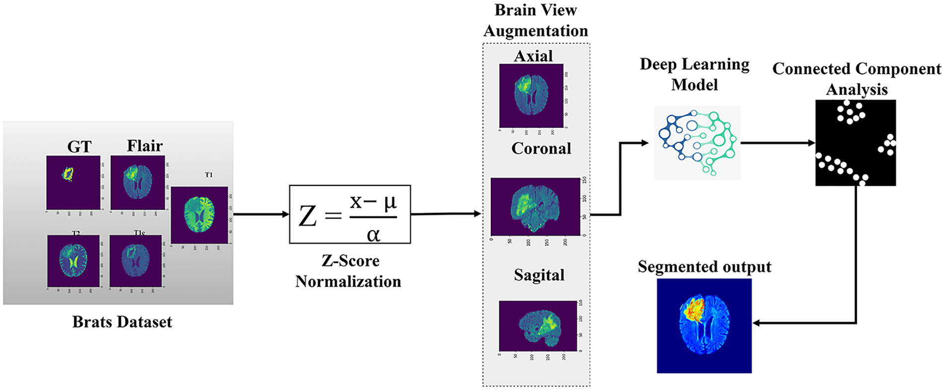
Figure 1: Overview of the methodology
In this study, all pixels contained small and essential information that must be captured for better segmentation. The inter-dilation factor, represented by
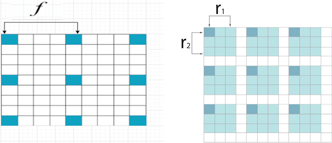
Figure 2: (a) Kronecker convolution with
This study used the 3DFSC network associated with a feature pyramid to generate hierarchical features of multi-scale intrinsic for segmenting tumors. The 3DFSC network learned the dense and non-destructive features of detailed lesions. The pyramid fused multi-scale features of lesions to handle tumors of various sizes. When the network got deeper, local features were preserved using skip connections to overcome the vanishing gradient, ensuring proper gradient flow within the network.
The contextual information supplied by these local features was sufficient to determine the boundaries of various lesion tissues. The contexts around the lesion became valuable auxiliary information to discriminate different tissues, including the cancerous and healthy cells. Each feature map in the network was combined using concatenation by aiming at learning the valuable features of the boundary to improve identifying the model for the anatomy of the lesion. Therefore, our network efficiently propagated complex and vital information without compromising essential data features. Our model segmented different cancerous lesions while preventing information loss with no increment in parameter numbers. Also, a single model was used to capture the contextual information from a multi-view for brain tumor segmentation. An adequate kernel size was used to address the varying tumor sizes among patients and different sizes of the tumor sub-region.
Also, this study has used feature maps to develop a 3D structure that helped multi-scale feature learning, as shown in Fig. 3. This block was added at the end of the 3DFSC network while KCFP fused the local and global features using a multi-input pyramid structure. Besides, the mapped features of the 3DFSC network were then propagated to each branch of the 3D Kronecker convolution with different intra–dilation and inter-dilation rates. Different dilatation rates were used at each pyramid level to generate three varying receptive fields for capturing multi-scale lesions. The small receptive field of this pyramid was responsible for segmenting the enhancing tumor, the medium for the non-enhancing tumor, and the large for the whole tumor. The last layer in our proposed model is the classification layer and it uses Multi-class Logistic Regression for segregating the classes. This regression based classification follow probability distribution between the range [0, 1].
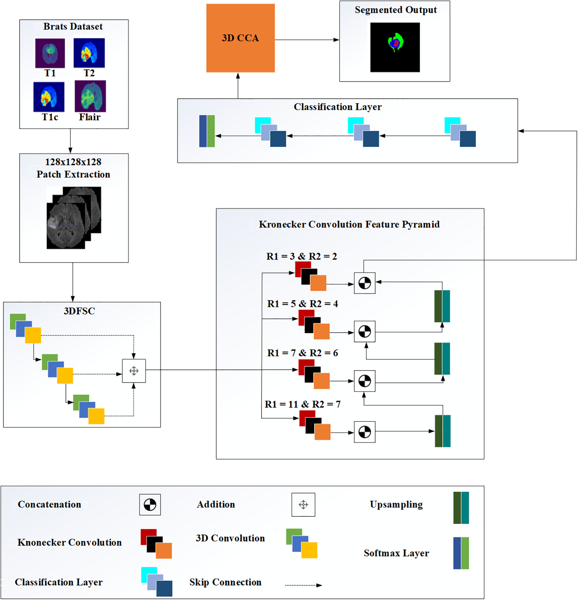
Figure 3: The architecture of the proposed methodology
Up-sampling layers were inserted to concatenate the feature maps at three different pyramid levels. Up-sample kept the dimension of each branch consistent with the previous one. This study also used an up-sample 3D block in the proposed pyramid learning mechanism to scale up the size of different feature maps without any learnable parameters. We also used Group Normalization (GN) for all layers in the network, further improving the performance of our model.
The performance of our segmentation model was evaluated using three metrics, i.e., dice similarity coefficient (DSC), sensitivity, and specificity. DSC metric was used for three labels, i.e., tumor core (TC), whole tumor (WT), and enhancing core (EC). WT and TC contained foreseen regions of EC, non-EC, and necrosis. However, WT had an additional prediction region, i.e., edema. The DSC metric was calculated using Eq. (2) [52].
where T is the manual label, P is the predicted region, |P| is the total area of P, |T| is the total area of T, and |P ∩ T| denotes the overlapped region between P and T.
Meanwhile, sensitivity is the proportion of correctly identified positives [5]. It was estimated using Eq. (3) [52].
where TP is the true positive and FN denotes the false negative. Specificity, the measure of the accurately identified proportion of actual negatives [7], was estimated using Eq. (4) [52].
where TN is the true negative and FP denotes the false positive. Also, the smaller the value, the closer the prediction of the actual value is calculated using Eq. (5).
where X is the volume of the mask, Y is the volume predicted by the model, and
Post-processing was performed to mitigate the impacts of false positives. Images were processed using the algorithm 3D Connected Component Analysis (CCA). This algorithm grouped the pixels into components based on the connectivity of the pixels to reduce false positives by removing outliers. Removing small, isolated clusters from the prediction results was essential because brain tumors were taken from the single connected domain.
Besides, the connected domain was analyzed to remove other small clusters. Some patients had benign tumors with gliomas consisting of non-enhancing and edemas tumors. In such a case, uncertainty arose when clusters of benign tumors were misclassified as enhancing tumors, causing inefficient segmentation. Therefore, volumetric constraints were imposed to remove enhancing tumors with values lower than the threshold. The 3D connected components were used to remove non-tumoral regions using a threshold. We experimented extensively with different pixels, i.e., 80, 100, 120, 150, 200, etc. Given that a global threshold of 500 pixels yielded the best prediction, all connected components smaller than this value were removed.
3.5 Training and Model Validation
We implemented our model with the PyTorch framework. For model training, the cross-validation evaluation of the training set is used. For validating the trained model, BraTs 2020 validation dataset was used. The patch size for training and validation was 128 × 128 × 128, containing most of the brain parts. This patch size was ideal for maximal information. Besides, we used the Adam optimizer with a learning rate of 0.001 and updated using the cyclic learning rate strategy after each iteration. For the brain tumor segmentation, we have utilized 3 million trainable parameters. Furthermore, we have trained our model with 400 epochs. Also, L2 regularization was used to prevent overfitting, while the Generalized Dice Loss function was used to resolve the class imbalance. Generalized Dice Loss is the cost function for our segmentation process, which is estimated using Eq. (6).
Meanwhile, Nvidia Titan X Pascal with NVIDIA Cuda core 3584 GPU was used to train the model for the experiments. Also, we measured the computational time of the network on NVidia Titan X Pascal with NVIDIA Cuda core 3584 GPU and Intel(R) Core(TM) M-5Y10c computer with a 1.80 GHz processor and 8 GB RAM.
The semantic segmentation process before and after the post-processing is shown in Fig. 4. Overall, segmented tumor boundaries became smooth and accurate after post-processing.
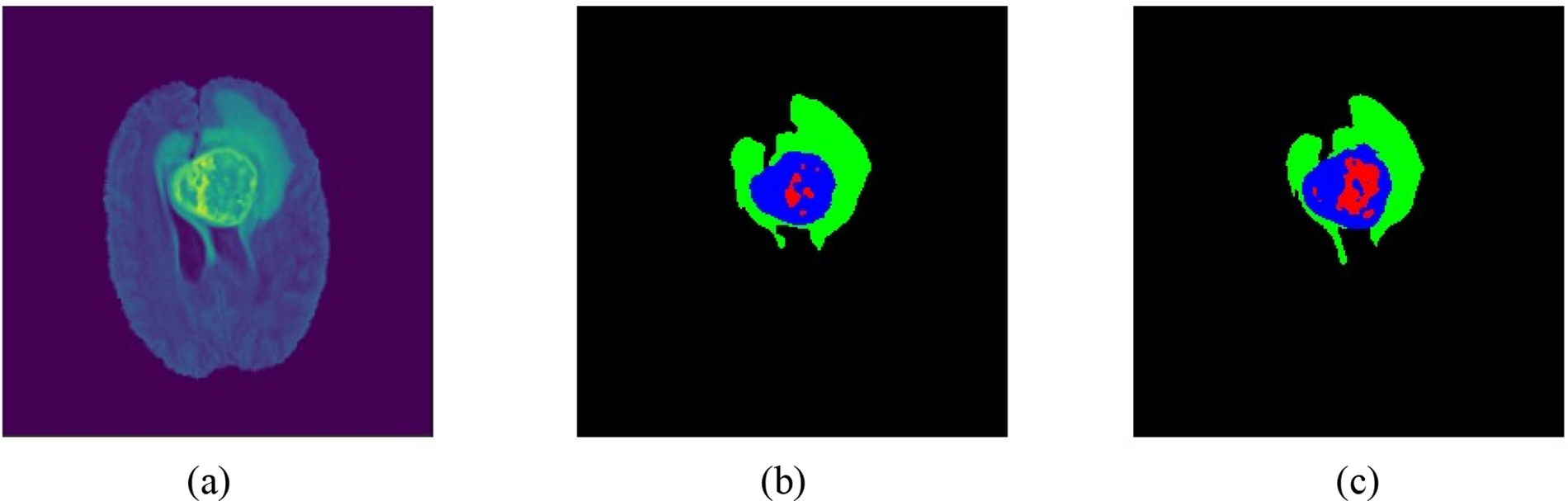
Figure 4: Patient samples from BraTs 2020 data: (a) brain volumetric MRI, (b) results before post-processing, and (c) results after post-processing
Table 2 shows the results of the evaluation with and without post-processing. Overall, post-processing enhanced efficiency.
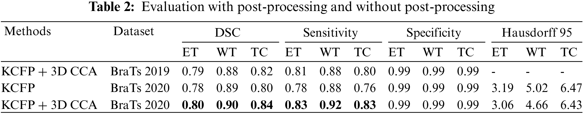
Table 3 compares the results of our KCFP model with the result of other benchmark schemes. The multilayer dilated convolutional neural network (MLDCNN) model [53] achieved a DSC of 0.76 on ET, 0.87 on WT, and 0.77 on TC. Its Hausdorff was promising compared to other methods. The Lesion encoder model used the spherical coordinate transformation as a pre-processing strategy to increase the accuracy of segmentation in combination with normal MRI volumes. It achieved a DSC of 0.71 on ET, 0.86 on WT, and 0.80 on TC [54]. Similarly, the ME-Net model used a multi-encoder for feature extraction with a new loss function known as Categorical Dice. It achieved a DSC of 0.73 on ET, 0.85 on WT, and 0.72 on TC. The AFPNet used a dilated convolution at multiple levels, fusing multi-scale features with context with a conditional random field as post-processing [55]. This model achieved a DSC of 0.71 on ET, 0.83 on WT, and 0.74 on TC. The AEMA-Net model achieved a DSC of 0.71 on ET, 0.83 on WT, and 0.74 on TC [56]. It used a 3D asymmetric expectation-maximization attention network to capture long-range dependencies for segmentation. The Transbts model exploited the transformer into 3D CNN using an encoder-decoder structure. It achieved a DSC of 0.76 on ET, 0.86 on WT, and 0.77 on TC [57]. The proposed model outperformed others in DSC, sensitivity, and Hausdorff 95. Our model achieved an average DSC of 0.80, 0.90, and 0.84 on the BraTs 2020 dataset for ET, WT, and TC, respectively.
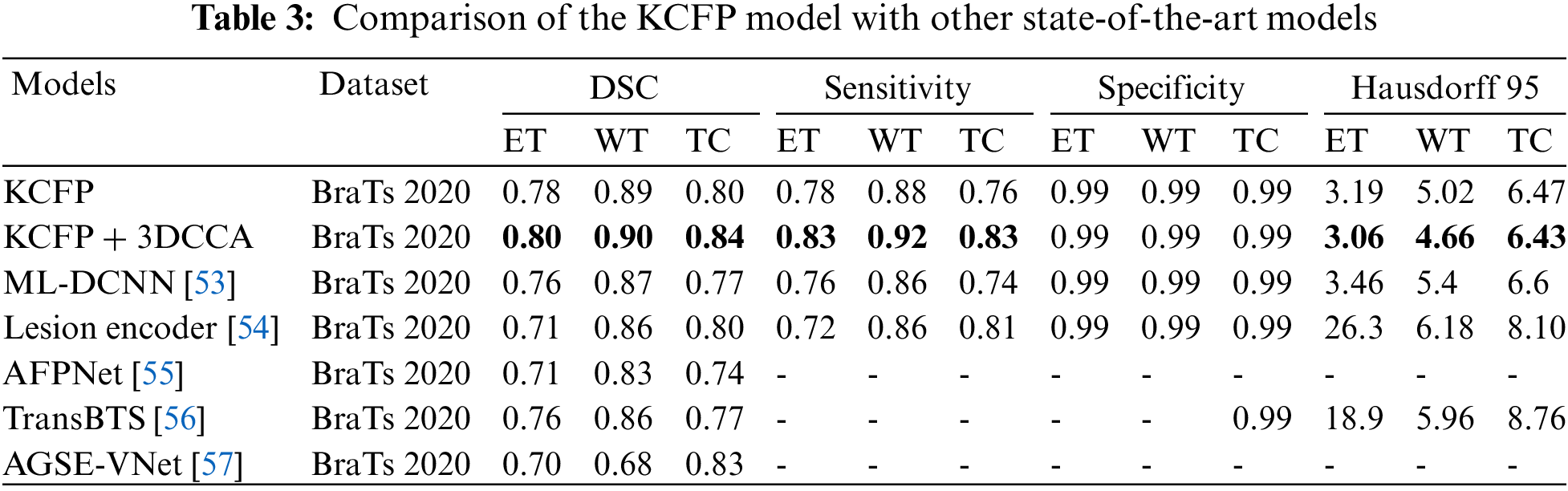
Fig. 5 shows the box plots of sensitivity, Hausdorff, and dice scores for three tumor regions. The dice score for the three tumor regions ET, TC, and WT are 0.80, 0.84, and 0.90, respectively (Fig. 5a). Based on the dice score, our model effectively improved the segmentation.
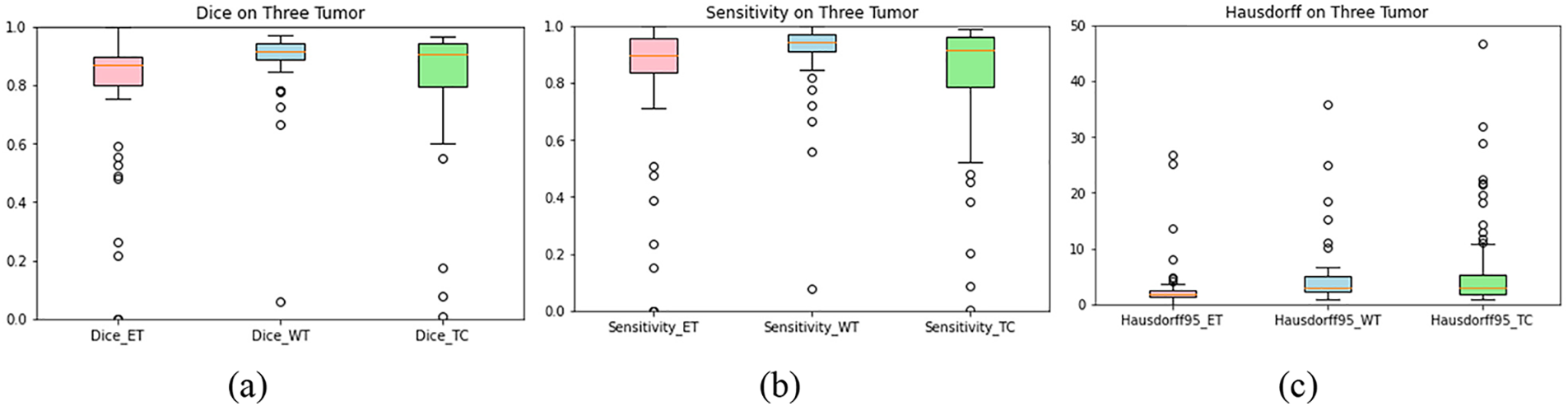
Figure 5: Plot-boxes: (a) dice score, (b) sensitivity, and (c) Hausdorff. The horizontal line in each box represents its median value. The hollow circle shows the outliers
Meanwhile, sensitivity reflects the impact of features on predicting models [58]. Fig. 5b shows that the sensitivity of our model is 0.83, 0.92, and 0.83 for ET, WC, and TC. Our KCFP model used size, location, and texture as features to identify the defective tissues, enhancing the final prediction that distinguished all healthy tissues from the damaged ones. Fig. 5c shows that the Hausdorff of our model is 3.06, 4.66, and 6.43 for ET, WC, and TC, respectively.
Fig. 6 shows the performance of the segmentation model with FLAIR-input MRI in three views: coronal, sagittal, and axial. The tumor predicted by our proposed model was very close to the ground truth, indicating that our model effectively segmented the brain tumors. The performance of segmentation of a patient taken from BraTs 2020 training set. The first column shows the brain MRI views, the second displays the ground truth labels, and the third depicts the predicted segmentation of patients using KCFP. The aquamarine-colored area represents a non-enhancing tumor, the red zone denotes enhancing tumor, and the dandelion-colored area indicates edema.
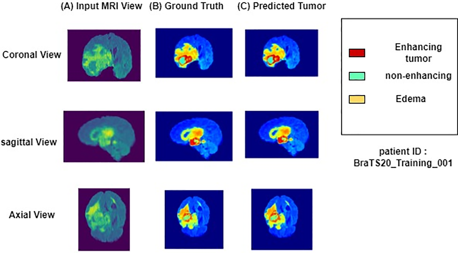
Figure 6: Results of a patient taken from BraTs 2020 training set
The automatic segmentation of brain tumors minimizes the burden of doctors while enhancing treatment planning for saving cancer patients [59]. However, the automatic segmentation of brain tumors faces many challenges due to the lesions’ different sizes, locations, and positions [60]. In this study, the problem of pixel loss in Atrous convolution caused by increased dilation rate was resolved using a 3D Kronecker convolution. The features lost in Atrous convolution were captured by Kronecker convolution. The 3D Kronecker convolution increased the receptive field while keeping the number of parameters constant and minimizing the pixel loss (Fig. 1). These pixels contained crucial information capturing, which was essential for better segmentation. The difference in intensity value and contrast in MRI volume was reduced by normalization [61]. The proposed model used the Kronecker-convolution feature pyramid to learn the characteristics of the lesion and preserve local features, thus improving the model’s capacity to distinguish TC from other lesions. The features learned by DCNN had multiple scales and nonlinear abstraction as a natural feature. This feature allowed the model to combine distinct hierarchies of abstract information, increasing the focus of the target areas [62]. The proposed model was trained with axial, coronal, and sagittal views. The multi-scale features of brain tumors were captured using 3D KCFP with various inter and intra-dilation factors. Lesion and context information was incorporated using this module to improve the segmentation.
The hierarchical features of multi-scale intrinsic generated by the 3DFSC network were used for effective and reliable segmentation. The 3DFSC learned the dense and non-destructive features of detailed lesions. Tumors of various sizes were handled using a feature pyramid. The vanishing gradient was resolved, and local features were preserved using skip connections from the 3DFSC network. This way, crucial and complex information was collected without losing essential data features. The proposed model was trained by providing all three possible brain views, i.e., axial, coronal, and sagittal. Besides, the feature maps at three different pyramid levels were concatenated using up-sampling layers. With the help of up-sampling, the dimension of each branch was kept consistent with each branch, further improving our model performance. The 3D CCA post-processing technique reduced false positives by combining the connected component analysis with a global threshold to remove outliers. Upon post-processing, tumor boundaries became smoother, effectively distinguishing the lesions from other tissues. Skip connections ensured the backpropagation of gradient flow to any layers without losing crucial information. Meanwhile, when evaluated using BraTs datasets, the proposed KCFP model of this study took 5 s on average to do segmentation for one patient. This average time was deemed reasonable. For future work, different inter-dilation and intra-dilation rates would be used to evaluate further and enhance our model performance.
In this study, a 3D KCFP was used for brain tumor segmentation to overcome the problem of pixel loss and weak processing of multi-scale lesions. The pixel loss was due to an increment in the dilation rate of Atrous convolution. We designed an integrated 3DFSC network with a multi-scale feature pyramid to learn local and global features interracially, overcoming the problem of weak processing. The 3DFSC learned the WT feature and its substructure effectively. By contrast, the feature pyramid dealt with multi-scale lesions. In this way, the proposed model distinguished the boundaries of various tumor tissues. Finally, false positives were reduced using the 3D CCA post-processing technique with a global threshold, attaining more structural segmentations. Our proposed model outperformed other benchmark schemes. Overall, our proposed KCFP model might benefit clinical medical image segmentation. However, the class imbalance problem is not completely mitigated in our proposed model. In the future, we will drive a cost function to solve the class imbalance problem completely and focus on different dilation rates to evaluate model performance.
Acknowledgement: This study was conducted at the Medical Imaging and Diagnostics Lab at COMSATS University Islamabad.
Funding Statement: This work was supported by “Human Resources Program in Energy Technology” of the Korea Institute of Energy Technology Evaluation and Planning (KETEP), granted financial resources from the Ministry of Trade, Industry & Energy, Republic of Korea (No. 20204010600090). In addition, it was funded from the National Center of Artificial Intelligence (NCAI), Higher Education Commission, Pakistan, Grant/Award Number: Grant 2(1064).
Author Contributions: All listed authors have substantially contributed to the manuscript and have approved the final submitted version. The authors confirm their contribution to the paper as follows:
• Kainat Nazir contributed to the literature review, design and development of AI-based architecture, the experimentation process, data collection, and manuscript writing.
• Tahir Mustafa Madni conceived the idea for the study and designed the overall research framework. He led the team throughout the entire experimentation process.
• Uzair Iqbal Janjua supervised data collection and performed in-depth data analysis to draw meaningful conclusions. He critically reviewed the experiment's outcomes in the context of existing literature, addressing potential implications and limitations of the AI models.
• Umer Javed contributed to the literature review to identify the gaps in knowledge and establish the context for our study.
• Muhammad Attique Khan guided the team throughout the study and provided overall leadership and expertise in this domain.
• Usman Tariq also actively participated in the interpretation and discussion of the results.
• Jae-Hyuk Cha performed in-depth data analysis, participated in discussion of the results, and critically reviewed the final version of the manuscript.
Availability of Data and Materials: A publicly available dataset was used for analyzing our model. This dataset can be found at http://ipp.cbica.upenn.edu.
Conflicts of Interest: The authors declare that they have no conflicts of interest to report regarding the present study.
References
1. A. Jose, S. Ravi and M. Sambath, “Brain tumor segmentation using k-means clustering and fuzzy c-means algorithms and its area calculation,” International Journal of Innovative Research in Computer and Communication Engineering, vol. 2, no. 3, pp. 3496–3501, 2014. [Google Scholar]
2. C. Ostgathe, “Differential palliative care issues in patients with primary and secondary brain tumours,” Supportive Care in Cancer, vol. 18, no. 2, pp. 1157–1163, 2010. [Google Scholar] [PubMed]
3. T. Saba, Z. Mehmood, U. Tariq and N. Ayesha, “Microscopic brain tumor detection and classification using 3D CNN and feature selection architecture,” Microscopy Research and Technique, vol. 84, no. 4, pp. 133–149, 2021. [Google Scholar] [PubMed]
4. A. Khan, A. Alqahtani, S. Alsubai and M. Alharbi, “Multimodal brain tumor detection and classification using deep saliency map and improved dragonfly optimization algorithm,” International Journal of Imaging Systems and Technology, vol. 10, no. 3, pp. 1–21, 2022. [Google Scholar]
5. N. Gordillo, E. Montseny and P. Sobrevilla, “State of the art survey on MRI brain tumor segmentation,” Magnetic Resonance Imaging, vol. 31, no. 8, pp. 1426–1438, 2013. [Google Scholar] [PubMed]
6. J. Liu, M. Li, J. Wang, F. Wu and Y. Pan, “A survey of MRI-based brain tumor segmentation methods,” Tsinghua Science and Technology, vol. 19, no. 6, pp. 578–595, 2014. [Google Scholar]
7. Z. P. Liang and P. C. Lauterbur, “Principles of magnetic resonance imaging: A signal processing perspective,” Institute of Electrical and Electronics Engineers Press, vol. 6, no. 2, pp. 1–21, 2000. [Google Scholar]
8. A. Drevelegas and N. Papanikolaou, “Imaging modalities in brain tumors,” Imaging of Brain Tumors with Histological Correlations, vol. 12, no. 2, pp. 13–33, 2011. [Google Scholar]
9. N. J. Tustison, “N4ITK: Improved N3 bias correction,” IEEE Transactions on Medical Imaging, vol. 29, no. 6, pp. 1310–1320, 2010. [Google Scholar] [PubMed]
10. L. G. Nyúl, J. K. Udupa and X. Zhang, “New variants of a method of MRI scale standardization,” IEEE Transactions on Medical Imaging, vol. 19, no. 2, pp. 143–150, 2000. [Google Scholar]
11. T. K. Behera and S. Bakshi, “Brain MR image classification using superpixel-based deep transfer learning,” IEEE Journal of Biomedical and Health Informatics, vol. 21, no. 6, pp. 1–10, 2022. [Google Scholar]
12. Z. Zhu, S. H. Wang and Y. D. Zhang, “RBEBT: A ResNet-based BA-ELM for brain tumor classification,” Computers, Materials & Continua, vol. 74, no. 2, pp. 101–111, 2023. [Google Scholar]
13. M. Masood, R. Maham, A. Javed and U. Tariq, “Brain MRI analysis using deep neural network for medical of internet things applications,” Computers and Electrical Engineering, vol. 103, no. 6, pp. 108386, 2022. [Google Scholar]
14. U. Zahid, I. Ashraf and K. M. Yahya, “BrainNet: Optimal deep learning feature fusion for brain tumor classification,” Computational Intelligence and Neuroscience, vol. 2022, no. 6, pp. 1–23, 2022. [Google Scholar]
15. F. Yu and V. Koltun, “Multi-scale context aggregation by dilated convolutions,” Sensors, vol. 6, no. 2, pp. 1–15, 2015. [Google Scholar]
16. M. I. Sharif, J. P. Li and U. Tariq, “M3BTCNet: Multi model brain tumor classification using metaheuristic deep neural network features optimization,” Neural Computing and Applications, vol. 6, no. 5, pp. 1–16, 2022. [Google Scholar]
17. Ö. Çiçek, A. Abdulkadir, S. S. Lienkamp and O. Ronneberger, “3D U-Net: Learning dense volumetric segmentation from sparse annotation,” in Medical Image Computing and Computer-Assisted Intervention–MICCAI 2016, Athence, Greece, pp. 424–432, 2016. [Google Scholar]
18. M. Irshad, M. Sharif and M. Yasmin, “Discrete light sheet microscopic segmentation of left ventricle using morphological tuning and active contours,” Microscopy Research and Technique, vol. 85, no. 2, pp. 308–323, 2022. [Google Scholar] [PubMed]
19. K. Kamnitsas, “Efficient multi-scale 3D CNN with fully connected CRF for accurate brain lesion segmentation,” Medical Image Analysis, vol. 36, no. 5, pp. 61–78, 2017. [Google Scholar] [PubMed]
20. D. Nie, L. Wang, E. Adeli, C. Lao and D. Shen, “3D fully convolutional networks for multimodal isointense infant brain image segmentation,” IEEE Transactions on Cybernetics, vol. 49, no. 3, pp. 1123–1136, 2018. [Google Scholar] [PubMed]
21. M. Havaei, P. M. Jodoin and H. Larochelle, “Efficient interactive brain tumor segmentation as within-brain kNN classification,” in 2014 22nd Int. Conf. on Pattern Recognition, NY, USA, pp. 556–561, 2014. [Google Scholar]
22. D. Yi, M. Zhou, Z. Chen and O. Gevaert, “3D convolutional neural networks for glioblastoma segmentation,” Applied Sciences, vol. 6, no. 5, pp. 1–14, 2016. [Google Scholar]
23. S. Iqbal, M. U. Ghani, T. Saba and A. Rehman, “Brain tumor segmentation in multi-spectral MRI using convolutional neural networks (CNN),” Microscopy Research and Technique, vol. 81, no. 4, pp. 419–427, 2018. [Google Scholar] [PubMed]
24. T. Wu, S. Tang, R. Zhang, J. Cao and J. Li, “Tree-structured kronecker convolutional network for semantic segmentation,” in 2019 IEEE Int. Conf. on Multimedia and Expo (ICME), NY, USA, pp. 940–945, 2019. [Google Scholar]
25. A. Hamamci and G. Unal, “Multimodal brain tumor segmentation using the tumor-cut method on the BraTS dataset,” in Proc. of MICCAI-BraTS, NY, USA, pp. 19–23, 2012. [Google Scholar]
26. E. Geremia, B. H. Menze and N. Ayache, “Spatially adaptive random forests,” in 2013 IEEE 10th Int. Symp. on Biomedical Imaging, NY, USA, pp. 1344–1347, 2013. [Google Scholar]
27. R. Meier, S. Bauer, J. Slotboom and M. Reyes, “Patient-specific semi-supervised learning for postoperative brain tumor segmentation,” in Medical Image Computing and Computer-Assisted Intervention–MICCAI 2014, Boston, USA, pp. 714–721, 2014. [Google Scholar]
28. K. Kushibar, “Automated sub-cortical brain structure segmentation combining spatial and deep convolutional features,” Medical Image Analysis, vol. 48, no. 6, pp. 177–186, 2018. [Google Scholar] [PubMed]
29. J. Bernal, “Deep convolutional neural networks for brain image analysis on magnetic resonance imaging: A review,” Artificial Intelligence in Medicine, vol. 95, no. 7, pp. 64–81, 2019. [Google Scholar] [PubMed]
30. J. Long, E. Shelhamer and T. Darrell, “Fully convolutional networks for semantic segmentation,” in Proc. of the IEEE Conf. on Computer Vision and Pattern Recognition, NY, USA, pp. 3431–3440, 2020. [Google Scholar]
31. A. Jesson and T. Arbel, “Brain tumor segmentation using a 3D FCN with multi-scale loss,” in Brainlesion: Glioma, Multiple Sclerosis, Stroke and Traumatic Brain Injuries, Quebec, Canada, pp. 392–402, 2018. [Google Scholar]
32. H. Shen, R. Wang, J. Zhang and S. J. McKenna, “Boundary-aware fully convolutional network for brain tumor segmentation,” in Medical Image Computing and Computer-Assisted Intervention−MICCAI 2017: 20th Int. Conf., Quebec City, QC, Canada, pp. 433–441, 2017. [Google Scholar]
33. F. Isensee, P. Kickingereder, W. Wick, M. Bendszus and K. H. Maier-Hein, “Brain tumor segmentation and radiomics survival prediction: Contribution to the brats 2017 challenge,” in Brainlesion: Glioma, Multiple Sclerosis, Stroke and Traumatic Brain Injuries, Quebec City, QC, Canada, pp. 287–297, 2018. [Google Scholar]
34. H. Dong, G. Yang, F. Liu, Y. Mo and Y. Guo, “Automatic brain tumor detection and segmentation using U-net based fully convolutional “Networks,” in Medical Image Understanding and Analysis: 21st Annual Conf., MIUA 2017, Edinburgh, UK, pp. 506–517, 2017. [Google Scholar]
35. J. Dolz, I. Ben Ayed and C. Desrosiers, “Dense multi-path U-net for ischemic stroke lesion segmentation in multiple image modalities,” in Brainlesion: Glioma,Multiple Sclerosis, Stroke and Traumatic Brain Injuries, Granada, Spain, pp. 271–282, 2018. [Google Scholar]
36. G. Kim, “Brain tumor segmentation using deep U-Net,” in Int. MICCAI BraTS Challenge, Quebec City, QC, Canada, pp. 154–160, 2017. [Google Scholar]
37. P. D. Chang, “Fully convolutional deep residual neural networks for brain tumor segmentation,” in Brainlesion: Glioma, Multiple Sclerosis, Stroke and Traumatic Brain Injuries, Athens, Greece, pp. 108–118, 2016. [Google Scholar]
38. F. Milletari, N. Navab and S. A. Ahmadi, “V-Net: Fully convolutional neural networks for volumetric medical image segmentation,” in 2016 Fourth Int. Conf. on 3D Vision (3DV), NY, USA, pp. 565–571, 2016. [Google Scholar]
39. A. Beers, “Sequential 3D U-Nets for biologically-informed brain tumor segmentation,” Sensors, vol. 4,no. 6, pp. 1–21, 2017. [Google Scholar]
40. G. Wang, W. Li, S. Ourselin and T. Vercauteren, “Automatic brain tumor segmentation using cascaded anisotropic convolutional neural networks,” in Brainlesion: Glioma, Multiple Sclerosis, Stroke and Traumatic Brain Injuries: Third Int. Workshop, BrainLes 2017, Held in Conjunction with MICCAI 2017, Quebec City, QC, Canada, pp. 178–190, 2017. [Google Scholar]
41. A. Casamitjana, M. Catà, I. Sánchez, M. Combalia and V. Vilaplana, “Cascaded V-Net using ROI masks for brain tumor segmentation,” in Brainlesion: Glioma, Multiple Sclerosis, Stroke and Traumatic Brain Injuries, Quebec City, QC, Canada, pp. 381–391, 2018. [Google Scholar]
42. X. Chen, J. H. Liew, W. Xiong and S. H. Ong, “Focus, segment and erase: An efficient network for multi-label brain tumor segmentation,” in Proc. of the European Conf. on Computer Vision (ECCV), NY, USA, pp. 654–669, 2018. [Google Scholar]
43. J. Liu, “A cascaded deep convolutional neural network for joint segmentation and genotype prediction of brainstem gliomas,” IEEE Transactions on Biomedical Engineering, vol. 65, no. 9, pp. 1943–1952, 2018. [Google Scholar] [PubMed]
44. O. Oktay, “Attention U-Net: Learning where to look for the pancreas,” Sensors, vol. 6, no. 5, pp. 1–23, 2018. [Google Scholar]
45. M. Noori, A. Bahri and K. Mohammadi, “Attention-guided version of 2D UNet for automatic brain tumor segmentation,” in 2019 9th Int. Conf. on Computer and Knowledge Engineering (ICCKE), NY, USA, pp. 269–275, 2019. [Google Scholar]
46. A. Sinha and J. Dolz, “Multi-scale self-guided attention for medical image segmentation,” IEEE Journal of Biomedical and Health Informatics, vol. 25, no. 1, pp. 121–130, 2020. [Google Scholar]
47. C. Chen, X. Liu, M. Ding, J. Zheng and J. Li, “3D dilated multi-fiber network for real-time brain tumor segmentation in MRI,” in Medical Image Computing and Computer Assisted Intervention–MICCAI 2019: 22nd Int. Conf., Shenzhen, China, pp. 184–192, 2019. [Google Scholar]
48. A. Roy Choudhury, R. Vanguri and P. Kumar, “Segmentation of brain tumors using DeepLabv3+,” in Brainlesion: Glioma, Multiple Sclerosis, Stroke and Traumatic Brain Injuries, Granada, Spain, pp. 154–167, 2019. [Google Scholar]
49. W. Zhang, “ME-Net: Multi-encoder net framework for brain tumor segmentation,” International Journal of Imaging Systems and Technology, vol. 31, no. 4, pp. 1834–1848, 2021. [Google Scholar]
50. G. Litjens, “A survey on deep learning in medical image analysis,” Medical Image Analysis, vol. 42, no. 3, pp. 60–88, 2017. [Google Scholar] [PubMed]
51. R. Ranjbarzadeh, A. Bagherian Kasgari and M. Bendechache, “Brain tumor segmentation based on deep learning and an attention mechanism using MRI multi-modalities brain images,” Scientific Reports, vol. 11, no. 1, pp. 1–17, 2021. [Google Scholar]
52. M. Ghaffari, A. Sowmya and R. Oliver, “Automated brain tumor segmentation using multimodal brain scans: A survey based on models submitted to the BraTS 2012–2018 challenges,” IEEE Reviews in Biomedical Engineering, vol. 13, no. 1, pp. 156–168, 2019. [Google Scholar] [PubMed]
53. K. Fiaz, “Brain tumor segmentation and multiview multiscale-based radiomic model for patient’s overall survival prediction,” International Journal of Imaging Systems and Technology, vol. 32, no. 3, pp. 982–999, 2022. [Google Scholar]
54. C. Russo, S. Liu and A. di Ieva, “Spherical coordinates transformation pre-processing in deep convolution neural networks for brain tumor segmentation in MRI,” Medical & Biological Engineering & Computing, vol. 60, no. 3, pp. 121–134, 2022. [Google Scholar]
55. Z. Zhou, Z. He and Y. Jia, “AFPNet: A 3D fully convolutional neural network with atrous-convolution feature pyramid for brain tumor segmentation via MRI images,” Neurocomputing, vol. 402, no. 5, pp. 235–244, 2020. [Google Scholar]
56. J. Zhang, Z. Jiang and B. Liu, “3D asymmetric expectation-maximization attention network for brain tumor segmentation,” NMR in Biomedicine, vol. 35, no. 5, pp. e4657, 2022. [Google Scholar] [PubMed]
57. W. Wang, C. Chen, M. Ding and J. Li, “Transbts: Multimodal brain tumor segmentation using transformer,” in Medical Image Computing and Computer Assisted Intervention–MICCAI 2021: 24th Int. Conf., Strasbourg, France, pp. 109–119, 2021. [Google Scholar]
58. S. Z. Kurdi, M. H. Ali, M. M. Jaber and R. Damaševičius, “Brain tumor classification using meta-heuristic optimized convolutional neural networks,” Journal of Personalized Medicine, vol. 13, no. 2, pp. 181, 2023. [Google Scholar] [PubMed]
59. V. Rajinikanth, S. Kadry and Y. Nam, “Convolutional-neural-network assisted segmentation and SVM classification of brain tumor in clinical MRI slices,” Information Technology and Control, vol. 50, no. 2, pp. 342–356, 2021. [Google Scholar]
60. S. Kadry, R. Damaševičius, D. Taniar and I. A. Lawal, “U-Net supported segmentation of ischemic-stroke-lesion in from brain MRI slices,” in 2021 Seventh Int. Conf. on Biosignals, Images, and Instrumentation (ICBSII), NY, USA, pp. 1–5, 2021. [Google Scholar]
61. S. Maqsood, R. Damaševičius and R. Maskeliūnas, “Multi-modal brain tumor detection using deep neural network and multiclass SVM,” Medicina, vol. 58, no. 8, pp. 1090, 2022. [Google Scholar] [PubMed]
62. S. Maqsood, R. Damasevicius and F. M. Shah, “An efficient approach for the detection of brain tumor using fuzzy logic and U-Net CNN classification,” in Computational Science and Its Applications–ICCSA 2021: 21st Int. Conf., Cagliari, Italy, pp. 105–118, 2021. [Google Scholar]
Cite This Article
 Copyright © 2023 The Author(s). Published by Tech Science Press.
This work is licensed under a Creative Commons Attribution 4.0 International License , which permits unrestricted use, distribution, and reproduction in any medium, provided the original work is properly cited.
 Downloads
 Citation Tools