A Multilevel Hierarchical Parallel Algorithm for Large-Scale Finite Element Modal Analysis

1  Introduction

Continuous development and research in engineering and scientific technology have brought the appearance of complex equipment and large or ultra-large systems [1,2]. The strict requirements of these systems in terms of safety and stability bring severe challenges to the numerical simulation of their dynamic system performance, which will result in large-scale DOFs in their finite element systems and make them difficult to solve [3–5]. Specifically, modal analysis is the most time-consuming link among all calculation processes of these complex dynamic systems and is also the basis for other calculations. High-precision modal analysis requires the help of large-scale finite element models, but these problems usually cannot get satisfactory solutions on traditional serial computers [6,7]. As a consequence, the research and development of corresponding large-scale modal analysis parallel algorithms can provide a feasible method for solving such problems on the basis of parallel supercomputers.

The mathematical essence of modal analysis can be eventuated to the large sparse matrix generalized eigenvalue problem. The solutions to these kinds of problems are often based on subspace projection techniques, which mainly include the Davidson subspace method and the Krylov subspace method. The Davidson subspace method is primarily applied in solving the eigenvalue of diagonally dominant symmetric matrices, but the applicability of this method is not as good as the Krylov subspace method [8,9]. The Krylov subspace method can be traced back to the 1950s with the proposed algorithms, including the Lanczos algorithm [10], the Arnoldi algorithm [11], the Krylov-Schur algorithm [12], etc. Later, worldwide researchers conducted a series of explorations on parallel algorithms of modal analysis based on the Lanczos algorithm, the Arnoldi algorithm, the Krylov-Schur algorithm, etc. The research mainly focused on two main types of parallel computing methods. One begins from the most time-consuming linear equations to seek the high-efficiency parallel computing method, and the other is from the finite element problem’s parallelism to form the modal synthesis method [13,14]. The direct and iterative approaches are the two fundamental algorithms for the parallel model solution of modal analysis. In terms of parallel computing of modal synthesis, researchers have combined direct and iterative methods. They started from the parallelism of the finite element problem itself, dividing the complex modal analysis problems into smaller sub-modal tasks for parallel processing. The direct method is used to solve the equations in sub-modal problems. The system-level modal GCEs after condensation are obtained through two modal coordinate transformations to reduce its overall scale. Then the iterative scheme is applied to solve the linear equations involved in the system-level modal GCEs after condensation. Therefore, the advantages of the direct method and iterative method can be well utilized to improve parallel efficiency, and thus it has been widely employed in the field of structural modal parallel computing. Rong et al. [15] designed a hybrid parallel solution for large-scale eigenvalues based on the modal synthesis algorithm (MSA) and transfer matrix method. Later, this method was applied to a vacuum vessel’s large-scale parallel modal analysis. Heng et al. [16] delivered a cantilever beam’s large-scale parallel modal solution on a shared memory parallel computer based on MSA. Aoyama et al. [17] improved the coupling method in the interfaces of each subsystem in MSA, and they successfully conducted the large-scale parallel modal analysis on a rectangular plate. Parik et al. [18] used the MSA to complete the design of the parallel modal analysis computing system based on OpenMP and utilized it in calculating the parallel modal analysis of a shaft system. Cui et al. [19] developed a simultaneous iterative procedure for the fixed-interface MSA, which has such merits as high computational efficiency, especially for reanalysis and parallel programming. However, when solving large-scale problems with the parallel modal synthesis approach (PMSA), with the increment in the number of subdomains, the scale and conditions of the system-level modal GCEs obtained after condensation also increase sharply, making it difficult to work out. Additionally, all processes need to participate in global communication when solving system-level modal GCEs with the iterative method. The overhead increment in inter-process communication and synchronization will greatly reduce the parallel efficiency.

In terms of hardware, the most widely used parallel computer in scientific and engineering computing is the distributed memory parallel computer, which architectures mainly include pure Central Processing Unit (CPU) homogeneous supercomputers [20] and heterogeneous supercomputers [21]. Particularly, heterogeneous supercomputers have become the mainstream architecture in distributed memory parallel computers due to their excellent computing power and cost-to-performance effectiveness. For heterogeneous distributed storage parallel computers, the most important parts are the different storage mechanisms in the cluster environment, the communication and cooperation between processors, and the load balance of the hardware architecture at all levels. These factors can also affect parallel efficiency significantly. Therefore, the keys to improving the parallel efficiency of heterogeneous distributed memory parallel computers are to balance the load between computing tasks and the hardware topology architecture of heterogeneous clusters, to ensure the storage of large-scale data, and to deal with the communication and cooperation between processors properly.

This paper focuses on providing a multilevel hierarchical parallel modal synthesis algorithm (MHPMSA) that is aware of the characteristics of heterogeneous multicore distributed storage computers and fully exploits their computing power to achieve optimal performance. The proposed algorithm, based on two-level partitioning and four transformation strategies, not only realizes the sparsely distributed storage of a large amount of data and speeds up the access rate of data memory but also reduces the scale of general GCEs after condensation effectively and saves the equation solution time. Moreover, this algorithm achieves a three-layer parallelization by utilizing the mapping between computational tasks and the hardware architecture of heterogeneous distributed storage parallel computers. And it can improve the load balance between different layers and accelerate communication efficiency by separating the communication between inter-nodes and intra-nodes, as well as the communication between HCGs and inside HCGs. There are various types of finite element methods, and this article targets the work of using heterogeneous distributed storage parallel computers to solve large-scale modal problems. It can be ported as a reference for other types of large-scale structural problems.

The rest of this paper is organized as follows: Section 2 introduces the related works of CPMSA to solve the large-scale modal analysis. Then, Section 3 describes the MHPMSA proposed with two-level partitioning, four-transformation strategies, and the implementation of MHPMSA with the best respect for the architecture of the ‘Shenwei’ heterogeneous multicore processor. In Section 4, two numerical experiments are presented. Finally, conclusions are drawn in Section 5.

2  Related Works

MSA can be divided into three categories according to the different processing methods of the DOFs of the substructure system interface: the free interface MSA [22], the fixed interface MSA [23], and the hybrid interface MSA [24], as shown in Fig. 1. In the MSA solution procedure, the low-order modal information of the substructure is used to represent the high-order modal information. When applying the free interface and the hybrid interface MSA, the existence of rigid body modes will cause the formation of singular stiffness matrices and cannot conduct matrix inversion. The fixed-interface MSA was first proposed by Tian et al. [25]. Its substructure modes include rigid body modes, constraint modes, and low-order modes of the fixed-interface substructure. Later, Craig and Monjaraz Tec et al. [26] improved the fixed interface MSA by controlling the additional constraints of the interface of the substructure system. Since the rigid body mode no longer needs to be considered in this method, the calculation process is simpler and has been widely used.

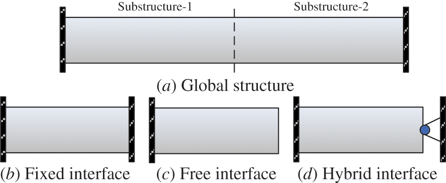
Figure 1: Three categories of MSA

The mathematical description of modal analysis is [27]:

Kφ=λMφ(1)

In this equation, K is the stiffness matrix of the overall modal system; M is the mass matrix of the overall modal system; λ is the generalized eigenvalue of the overall modal system; φ is the corresponding mode shape vector. K and M are all large sparse, symmetric positive (semi) definite matrices and can be obtained through the finite element discretization and integration of the engineering system structures. The essence of modal analysis is to solve multiple low-order eigenpairs of Eq. (1).

The finite element mesh is divided once in the conventional parallel modal synthesis algorithm (CPMSA), as shown in Fig. 2. There are two meshing algorithms: 1D algorithm and 2D algorithm. Compared with the 1D algorithm, the 2D algorithm is more suitable for models with extremely large DOFs or with complicated configurations [16,28]. According to the numbering principle, the generated m sub-regions first settle the internal DOFs for the I set and then settle the boundary DOFs B set. The mass matrix Msub and the stiffness matrix Ksub of each sub-domain system can be expressed as:

[Ksub]=[KIIKIBKBIKBB]; [Msub]=[MIIMIBMBIMBB](2)

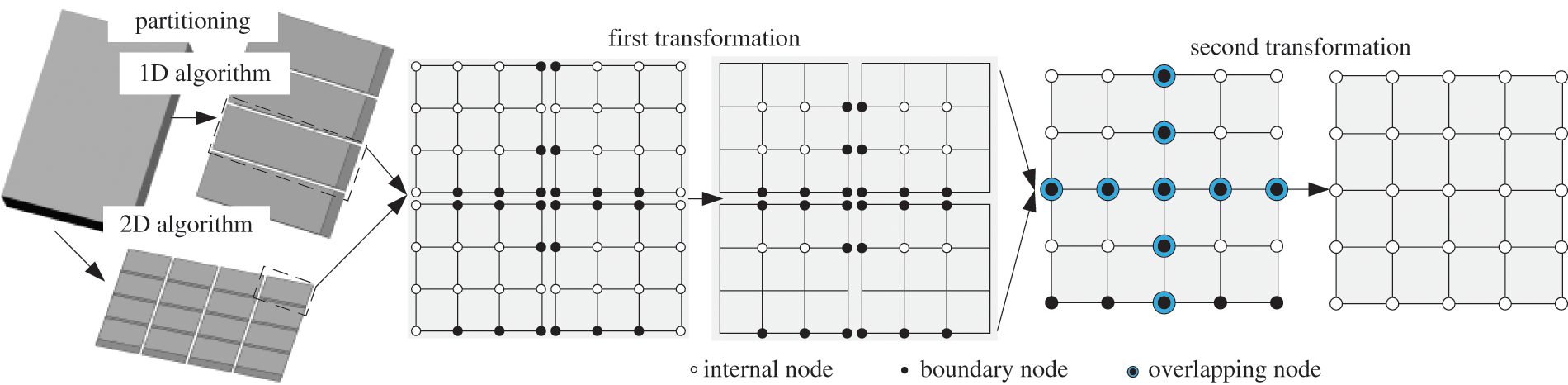
Figure 2: Partitioning and transformation of CPMSA

When performing the first coordinate transformation, the relationship between the physical coordinates of each sub-domain system and the modal coordinates can be expressed as:

[UIUB]=[Φ][pkpB]≈[ΦIkΨIB0BKIBB][pkpB](3)

In the formula, UI and UBrepresent the displacements of the internal nodes and boundary nodes, respectively. [IBB] is the identity matrix, [0BK] is a zero matrix, {pk} is the k modal coordinates corresponding to the internal nodes, and {pB} is the l modal coordinates corresponding to the boundary nodes. [Φ] is the modal transformation matrix of each substructure, and [ΦIk] is the principle modal matrix formed by internal nodes. (KII, MII) can construct GCEs and take the eigenvector group formation corresponding to the first k low-order eigenvalues, as Eq. (4) shows. [ΦIk] is the constrained mode and can be calculated as Eq. (5).

KIIφI=λIMIIφ(4)

ΨIB=−[KII]−1[KIB](5)

The condensed equivalent stiffness matrix [K~] and equivalent mass matrix [M~] of each sub-domain are:

[K~]=[Φ]T[K][Φ],[M~]=[Φ]T[M][Φ](6)

The second coordinate transformation is performed as shown below by utilizing the displacement coordination conditions among the sub-domain systems:

[p~]=[S][q~](7)

In the equation, [p~] is the modal coordinates corresponding to the boundary nodes and internal nodes of the set in each sub-domain system as shown in Eq. (8). In Eq. (7), [S] is the independent modal coordinate transformation matrix. [q~] is the independent modal coordinate obtained after removing the modal coordinate of boundary notes in the repeat set.

[p~]=[[pk0,pB0−j1,…,pB0−jj],…,[pkm,pBm−k1,…,pBm−kk]]T(8)

[q~]=[p~]−{{pBjk}|{pBjk}∈[q~] and exist {pBkj}∈[q~]}(9)

Transform the equivalent stiffness matrix and the equivalent mass matrix after simultaneous all sub-domains, and we can get the reduced GCEs for the whole system:

K∗φ∗=λ∗M∗φ∗(10)

The reduced stiffness matrix [K∗] and the reduced mass matrix [M∗] are:

[K∗]=[S]T[K′~][S],[M∗]=[S]T[M~][S](11)

Employing the parallel Krylov subspace iteration method to solve Eq. (10) can get the low-order modal frequencies and mode shapes required by the overall system, and substituting it into Eq. (3) can obtain the mode shapes of each sub-structure.

3  Proposed MHPMSA Based on Shenwei Multicore Processor Architecture

MHPMSA, based on two-level partitioning and four-transformation strategies and sparsely distributed data storage, not only improves the load balancing of different levels through parallel task mapping but also realizes communication separation and effectively improves communication efficiency. Furthermore, it reduces the scale of the system-level modal generalized characteristic and saves the iterative convergence time.

3.1 Proposed MHPMSA

To reduce time in condensing sub-domains, assembling and solving the system-level modal GCEs in sub-domains level 1 with the increasing number of sub-tasks, MHPMSA war proposed on the basis of two-level partitioning and four-transformation strategies.

In the two-level partitioning, the initial mesh of finite element is first partitioned into p level 1 subdomains with the 2D algorithm on the basis of ParMetis [29]. Then, every level 1 subdomain is divided into m level 2 subdomains on the basis of the characteristics of heterogeneous multicore architecture, which adapts to the heterogeneous multicore distributed storage supercomputer, ‘Shenwei-Taihuzhiguang’. Where p should be the total number of starting node machines in parallel computing, and m represents the number of HCGs in a single node machine, which is 4. For example, as shown in Fig. 3, if p is equal to 2, then the meshing of the finite element will be divided into two level 1 sub-domains at first, and then every level 1 subdomain is partitioned into four level 2 subdomains again.

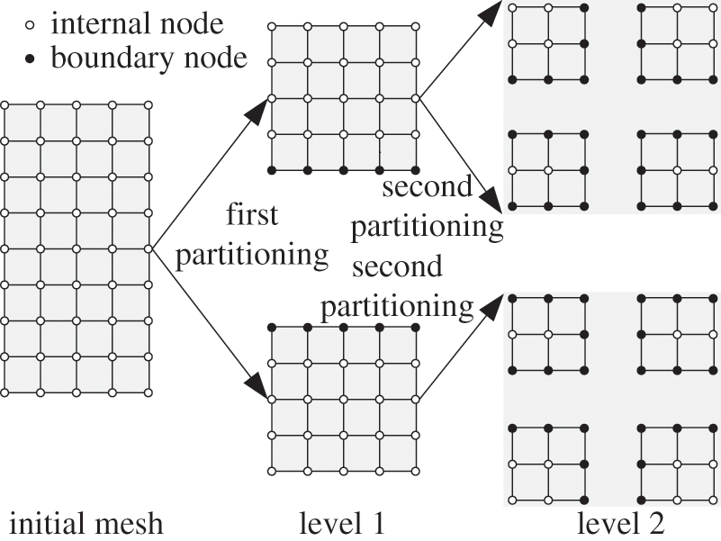
Figure 3: Two-level partitioning

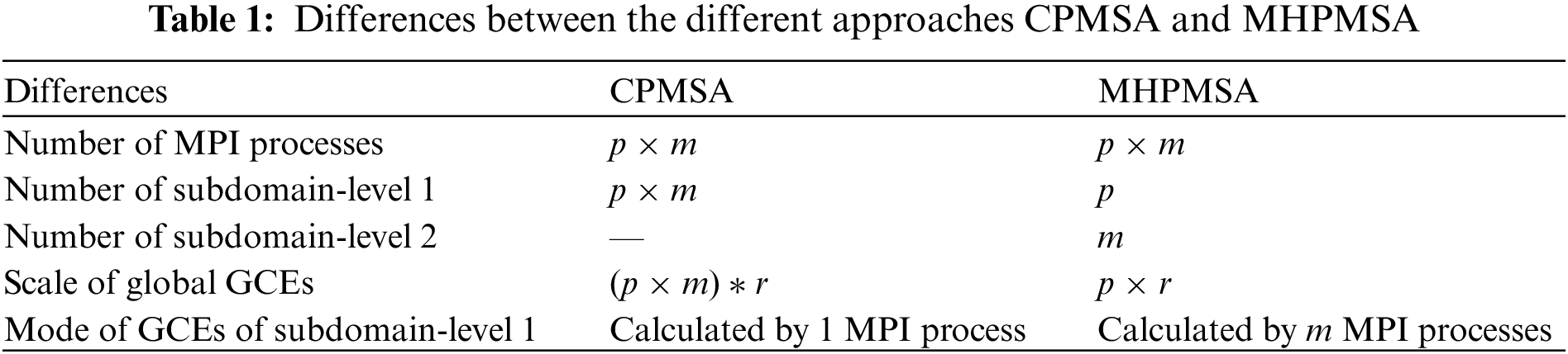
The four-transformation recognizes the transformation process by successfully applying Eqs. (3) and (7) on levels 1 and 2 subdomains, as shown in Fig. 4. Firstly, it will form the mass and stiffness matrixes for every level 2 subdomain. Then, throughout the first coordinate transformation, it will constitute the GCEs that only contain internal freedom. Later, the equivalent stiffness and mass matrices are calculated by condensation in each subdomain. Then, by grouping all equivalent stiffness and mass matrices of level 2 subdomains within the same level 1 subdomain and applying the second coordinate transformation can gain the GCEs of level 1 subdomains that only contain independent coordinates. After series condensations, grouping, and coordinates transformations according to Eqs. (7)∼(11), we can get the GCEs of the whole system only involving independent coordinates. Then, global GCEs can be solved by the parallel Krylov subspace iteration method to determine the low-order modal frequencies and mode shapes required by the overall system. Finally, modal frequencies and mode shapes of each sub-structure can be calculated by parallel back substituting according to Eq. (3). The differences between the different approaches CPMSA and MHPMSA are shown in Table 1.

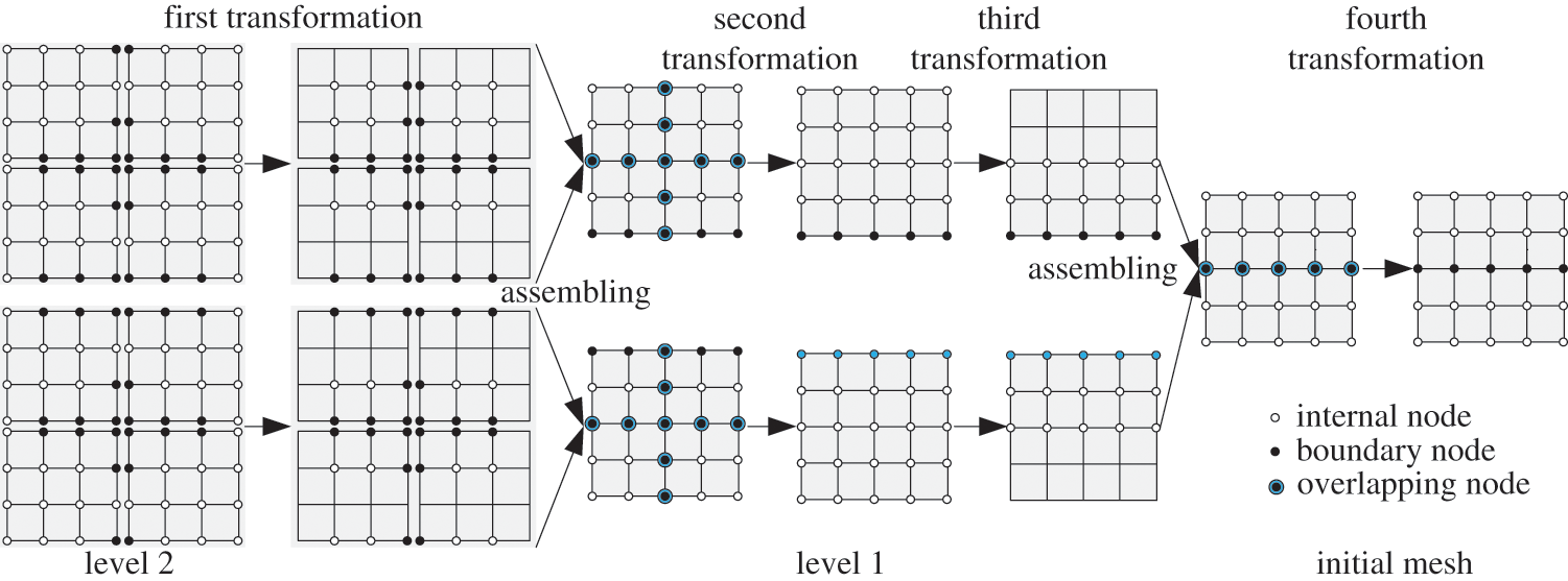
Figure 4: Four transformations

3.2 Architecture and Execution Mode of Shenwei Multicore Processor

Heterogeneous supercomputers are usually equipped with multicore CPUs, Graphics Processing Unit (GPUs), Many Integrated Cores (MIC) processors, or heterogeneous groups to calculate the computational tasks together. For example, the APU project by AMD company [30], the Echolen project led by NVIDIA company [31,32], the Runnemede project conducted by Intel company, and Wuxi-Hending company’s project named ‘Shenwei-Taihuzhiguang’ [1] in this article, etc.

Because there are a wide variety of heterogeneous multicore supercomputers, this paper mainly focuses on the parallel solution of large-scale modal problems using the ‘Shenwei-Taihuzhiguang’ supercomputer to analyze and solve the problem in a targeted manner. ‘Shenwei-Taihuzhiguang supercomputer is built based on ‘Shenwei’ multicore processor architecture, as shown in Fig. 5. There are four HCGs in every Shenwei heterogeneous multicore processor, and all four of these HCG shares 32 GB memory. Every HCG owns one main core (computational control core) and 64 computing cores (computing core array). To ensure the implementation of MHPMSA with the best respect for the architecture of the ‘Shenwei’ heterogeneous multicore processor, each node should make full use of all four HCGs in parallel computing. And every HCG should make full use of the main core and 64 computing cores. Besides, all of ‘Shenwei’ multicore processors are not in any particular order of importance. The principle of network among ‘Shenwei’ multicore processors adopts peer-to-peer network communication protocol. Hence, the number of ‘Shenwei’ multicore processors can be arbitrarily selected without consideration of the parallel efficiency and the storage of large-scale data.

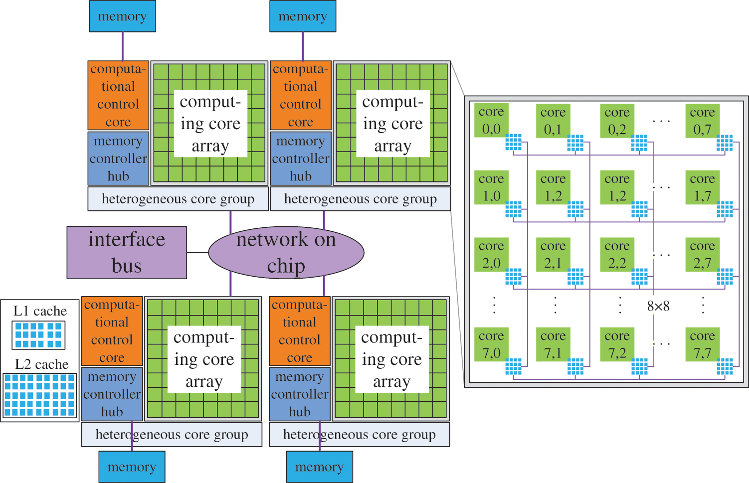
Figure 5: Shenwei multicore processor architecture

The communication between the HCGs adopts the bidirectional 14 G bits/s bandwidth. And the communication between the computational control and the computing core adopts the DMA method to get bulk access to the main memory. The local storage space of the computing core is 64 KB, and the command storage space is 16 KB. The features of its communication are: the communication efficiency of the intra-node is much higher than that of the inter-node. Similarly, the communication rate within the same HCG is much greater than that between the HCGs.

3.3 Parallel Task Mapping

Considering the features of communication on Shenwei multicore processor architecture, the keys to improving the parallel efficiency of large-scale finite element modal analysis of heterogeneous distributed memory parallel computers are: (1) to balance the load between computing tasks and the hardware topology architecture of heterogeneous clusters; (2) to ensure the storage of large-scale data and (3) to deal with the communication and cooperation between processors properly. Through mapping, the computing tasks to different hardware layers of heterogeneous multicore supercomputers can achieve load balancing among different layers and accomplish efficacious partitioning in communication [33].

Based on the CPMSA and considering the hardware architecture of the heterogenous multicore supercomputer ‘Shenwei-Taihuzhiguang’, we formed the task mapping of MHPMSA for structural large-scale modal analysis, as shown in Fig. 6.

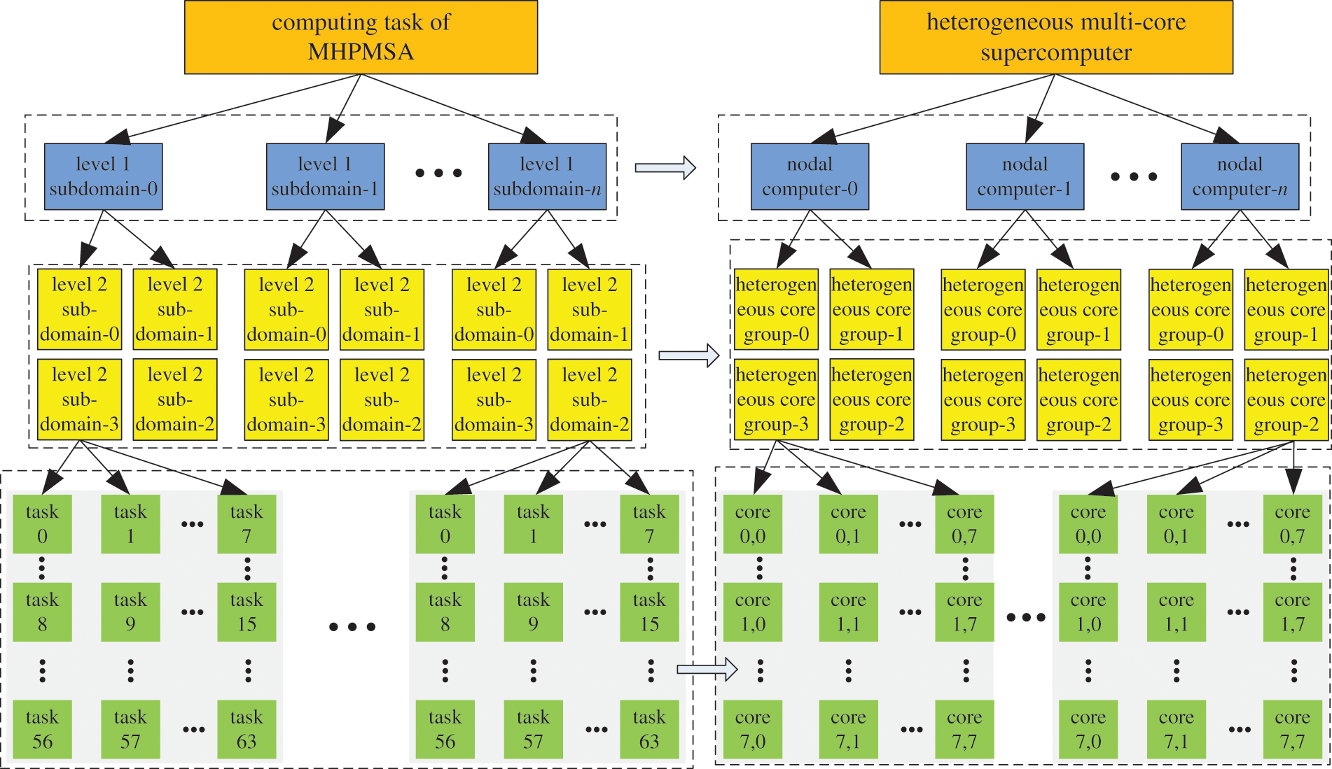
Figure 6: Task mapping of MHPMSA for structural large-scale modal analysis

When performing task mapping, the level 1 mesh subdomains are mapped according to the order of nodes, and the level 2 mesh subdomains are mapped according to the heterogeneous groups within nodes. The floating-point operations in each HCG are mapped in agreement with the computing cores.

‘Shenwei’ heterogeneous multicore processor is configured with 8G private memory and can be accessed independently. Therefore, to speed up the memory access rate during the calculation, the data and information of each subdomain are stored in its corresponding HCG within the node machine through multiple file streams. Besides, compared to the CPMSA, the MHPMSA further reduces the scale of the overall GCEs of the system and accelerates its iterative convergence speed with two-level partitioning and four transformation strategies.

3.4 The Three-Layer Parallelization Computational Mechanism

Based on the communication characteristic of heterogeneous multicore distributed storage parallel computers, the key to improving communication efficiency lies in realizing the communication separation between inter-nodes and intra-nodes, also the communication between different HCGs and inside HCGs when controlling the communication cooperation. As well as reduce the communication and synchronization overheads generated in the whole solution procedure of the system. That is, according to the communication architecture of the heterogeneous multicore distributed parallel storage computer, to restrict the large amount of local communication within the intra-nodes. And minimize the global communication in inter-nodes at the same time. The MHPMSA just satisfies these conditions. As shown in Fig. 7, it realizes the three-layer parallelization computation based on the two-level partitioning and four-transformation approach mentioned before.

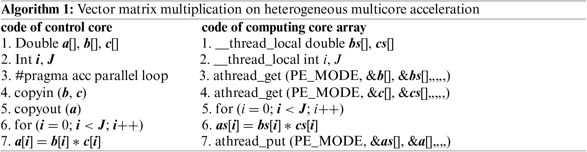
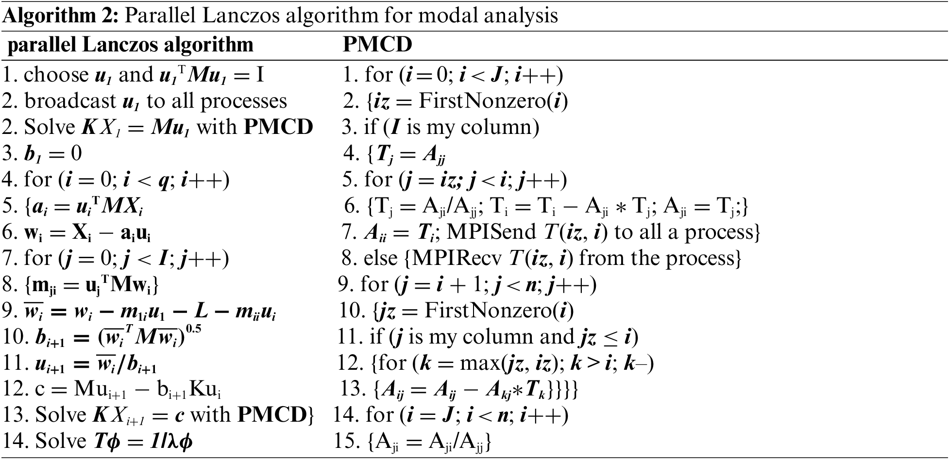
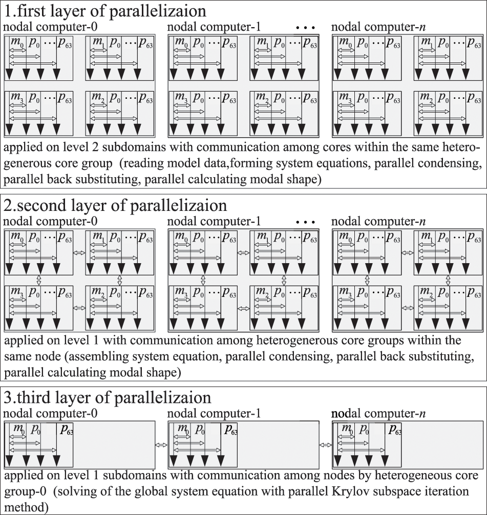
Figure 7: Scheme of three-layer parallelization for large-scale finite element modal analysis

First-layer parallelization: In the first-layer parallelization, the m processes of each node are responsible for the processing procedure corresponding to the level 2 subdomain system. All processes operate synchronously, and there is no data interaction between different processes. In the process, data interaction exists between the computing control core and the computing core array. The maximum amount of data that can be used in one data interaction between the computing control core and a single computing core is 64 KB. The data processing processes include: the computing control core of each HCG reading the model data of the subdomain; each computing control core carrying out the calculations corresponding to the computing core array to form the equivalent stiffness matrix Ksuband an equivalent mass matrix Msubof their subdomain; applying the parallel Lanczos method to solve the equivalent stiffness matrix [K~] and equivalent mass matrix [M~], which are calculated through level 2 GCEs (KII, MII) after condensation, and solving the mode shapes of level 2 subdomain though back substituting. Since these computing processes are operated based on unit information, each process can be performed independently according to the system information of the level 2 subdomain. Therefore, there is no need for data to interact between processes, and the data interactions only exist between the computing control core and the computing core array.

To save memory space and to reduce the amount of calculation, the local overall stiffness matrix and mass matrix of each level 2 subdomain are stored with the compressed sparse column technique. The matrix-vector operations involved in Eqs. (2)∼(9), mainly including addition, subtraction, multiplication, and division, are performed with the Athread library. Take the vector multiplication a = b × c as an example (a, b, and c are the storage arrays in any matrix-vector operation procedure); its operation is shown in Algorithm 1. The 64 computing cores on each HCG read the corresponding data from its memory space synchronously and cyclically. The required memory in this data segment should be less than 64 kb. After calculation, the data will return to specific locations. Communication only exists between the computing control and the computing core in the process.

Second-layer parallelization: Each node machine simultaneously performs the set of the corresponding level 1 subdomain, the parallel condensation, and back substituting. Communication exists between different HCGs within the same node and in each HCG between the control core and the compute core. The data in the calculation process adopts the compressed sparse column technique for distributed storage. During calculation, the No. 0 HCG in each node machine is responsible for summarizing the results and the internal back substituting and solutions of the set, data distribution, and parallel consideration. At the same time, all HCGs in the same node machine will participate in the parallel computational procedure corresponding to the level 1 subdomain within every node machine. The parallel Lanczos method is applied to solve the GCEs (KII, MII) of the level 1 subdomain. And the linear equations involved in the procedure are preprocessed through the parallel modified Cholesky decomposition (PMCD), as shown in Algorithm 2.

Third-layer parallelization: The parallel Krylov subspace iteration method is used here to solve the reduced GCEs of the whole system. Every node machine only has one core group, named No. 0 HCG, to join in the solution and communication, as shown in Fig. 8. During the solution, the overall reduced stiffness matrix and reduced mass matrix of the system are still stored distributively in the memory space corresponding to the No. 0 HCG. The intermediate calculation results also employ the compressed sparse column technique for distributed storage. Consequently, a large amount of local communication is limited between the computing control core and the computing core array of each HCG. And only a few dot product operations and computations for overall iterative errors need global communication. Therefore, it can effectively reduce the amount of communication and improve parallel computing efficiency.

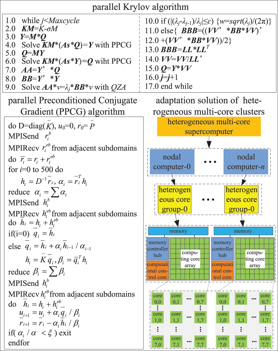
Figure 8: Parallel Krylov algorithm and task mapping

In summary, MHPMSA can confine a considerable amount of local communication within every node machine while ensuring that every node machine has one HCG, which is the No. 0 HCG, to participate in global communication. This strategy realizes the communication separation of intra-node and inter-node, reducing the communication and cooperation overheads in the computational procedure. As a consequence, the MHPMSA can significantly improve communication efficiency.

4  Numerical Study and Discussion

4.1 Numerical Experiments

The ‘Shenwei-Taihuzhiguang’ supercomputer is used to verify the correctness and effectiveness of the proposed algorithm. Each node starts using four HCGs during the test. And every HCG starts using one main core and 64 computing cores with 8 GB memory. The proposed algorithm and the CPMSA are used in the modal analysis of a disc brake rotor in an ultra-deep drilling rig. The FEM mesh model is shown in Fig. 9. The elastic modulus assigned to the model is 210 GPa, and the density is 7800 kg/m3, and the Poisson’s ratio of 0.3. Applying different DOFs scales and setting fixed constraints on the 8 bolt-hole positions on the inner surface. The structural first 20 natural frequency results are calculated and compared with the results computed by the Lanczos algorithm [10,34]. The test scales are shown in Table 2, and the maximum relative errors of the first 20 natural frequencies of each test scale are calculated by Eq. (12), and the results are shown in Fig. 10.

εm=||λ−λlanczos||2||λlanczos||2(relative errors)(12)

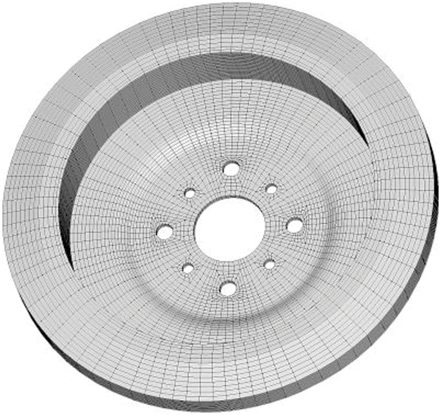
Figure 9: FEM of brake system on an ultra-deep drilling rig

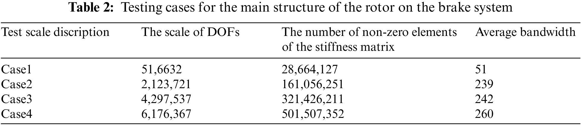
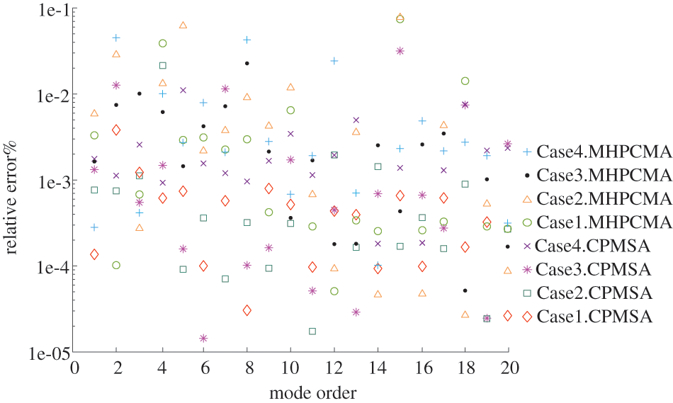
Figure 10: The modal relative errors for different DOFs

To reveal the necessity of large-scale modal calculation of complex systems, we conduct comparative analyses of the modal frequency results of Case1∼Case4. Table 3 shows the comparison of modal frequencies under four different scales. And the source of the original experimental data of Table 3 is the modal frequency for different scales of the rotor on the brake system, which is calculated by the Lanczos algorithm.

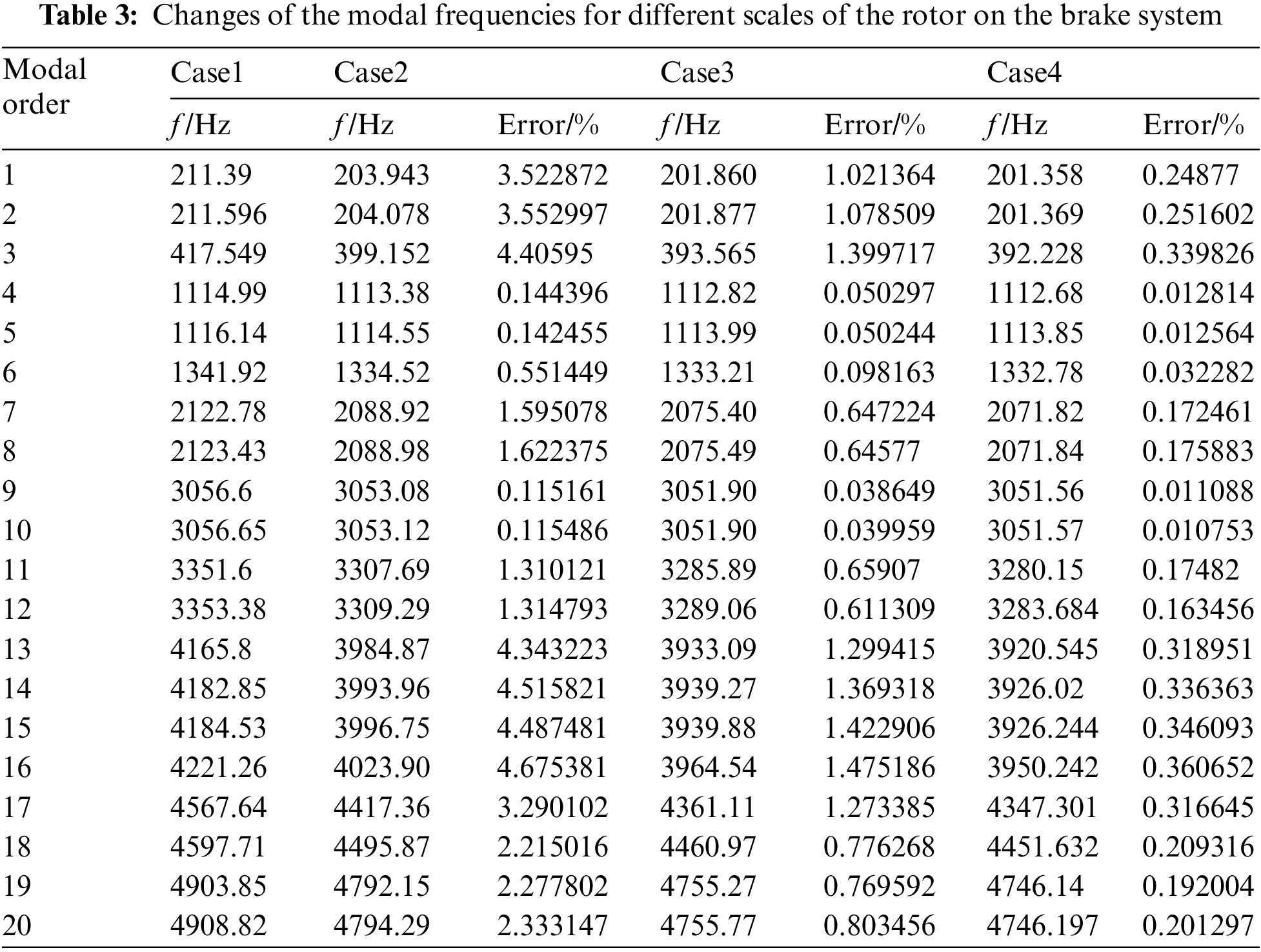
From Table 3, it can be seen that with the increase in the calculation scale, the modal frequency of each order will gradually decrease. This pheromone is caused by the ‘hardening effect’ of stiffness matrices in complex systematic finite element analysis, and it will cause a higher modal frequency in a relatively small DOFs calculation scale. Compared with the modal frequencies of Case1∼Case3, the maximum rate of change is 4.68%, while for the modal frequencies of Case3 to Case4, the rates of change are much lower, indicating that for the finite element analysis of complex systems, it is necessary to increase the corresponding calculation scale to improve its accuracy.

For a special problem, if the available nodes for parallel computing range from i to j (0 < i < j <…< p), and the corresponding time costs are (t0, ti, tj,…, tp), respectively. Then, the speed up of parallel computing with j cores is calculated by Eq. (13). And the corresponding parallel efficiency is calculated by Eq. (14).

Sj=titj(j=i,…,p)(13)

Ei=hSii×100%(j=i,…,p)(14)

The MHPMSA proposed in this article and the CPMSA are tested by starting the corresponding number of node machines. With the consideration of features of the ‘shenwei’ multicore processors and the storage of large-scale data, the total number of startup node machines in sequence during the test is 16, 32, 64, and 128. Since the total number of level 1 subdomains in two-level partitioning should be equal to the total number of start node machines, the number of corresponding level 1 domains should be 16, 32, 64, and 128 as well. Every node of ‘Shenwei-Taihuzhiguang’ supercomputer contains 4 HCGs, and thus in the second partition, every level 1 domain will be divided into 4 independent level 2 domains. The parallel calculation results of Case2 to Case4 are shown in Tables 4∼6. The source of the original experimental data of Tables 4∼6 is the solution time for different scales, which is calculated by CPMSA and MHPMSA with different numbers of node machines. Then, the speedup and parallel efficiency can be calculated by Eqs. (13) and (14).

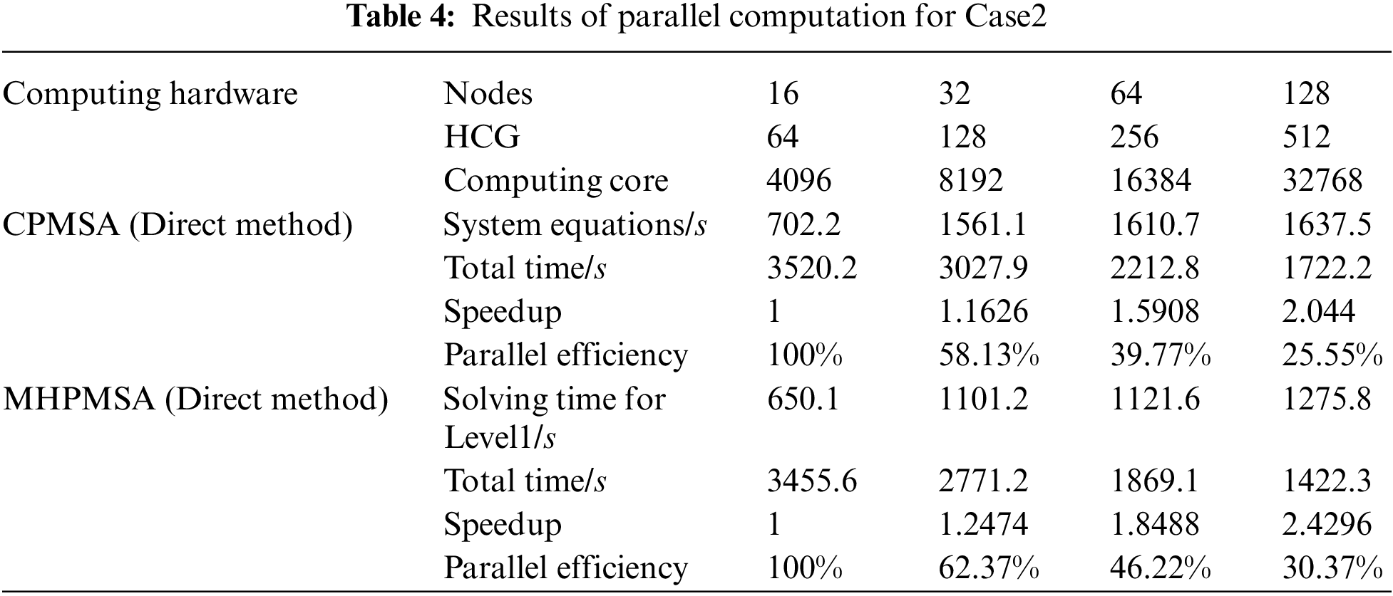
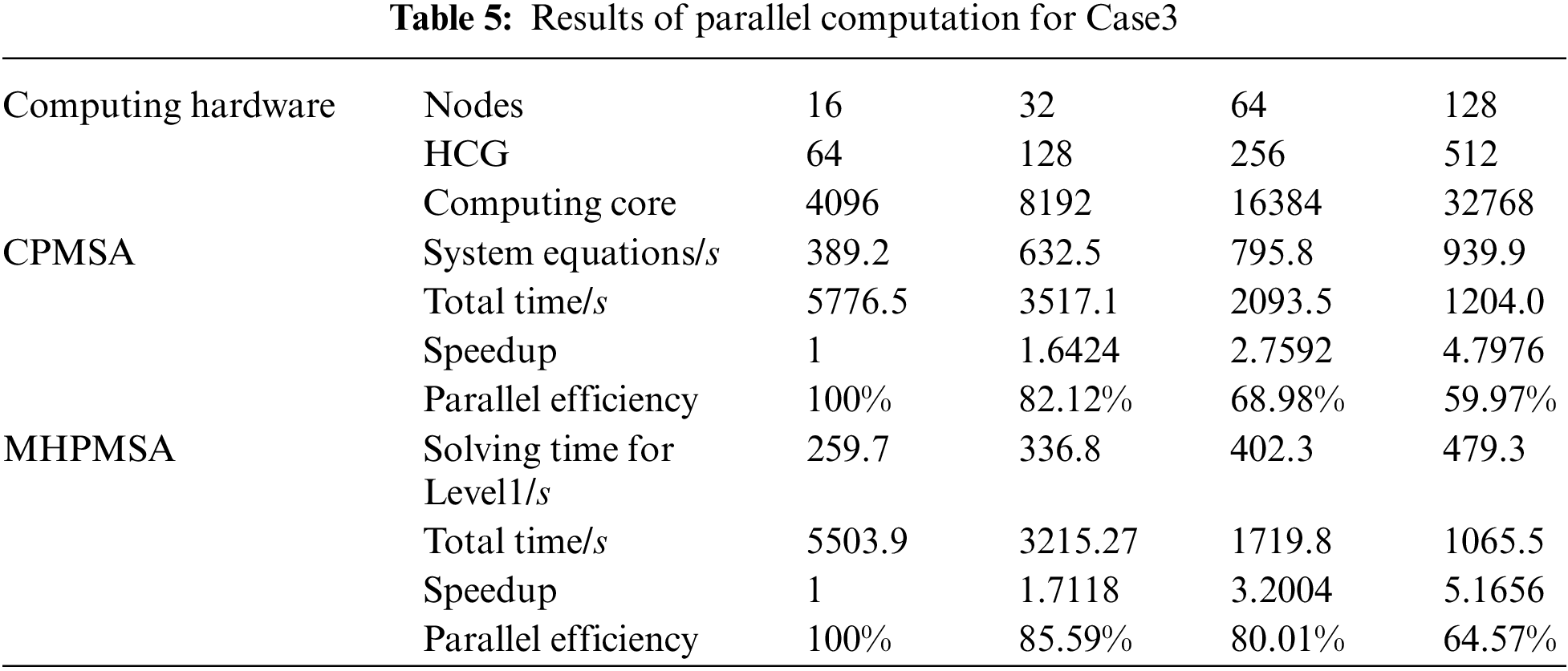
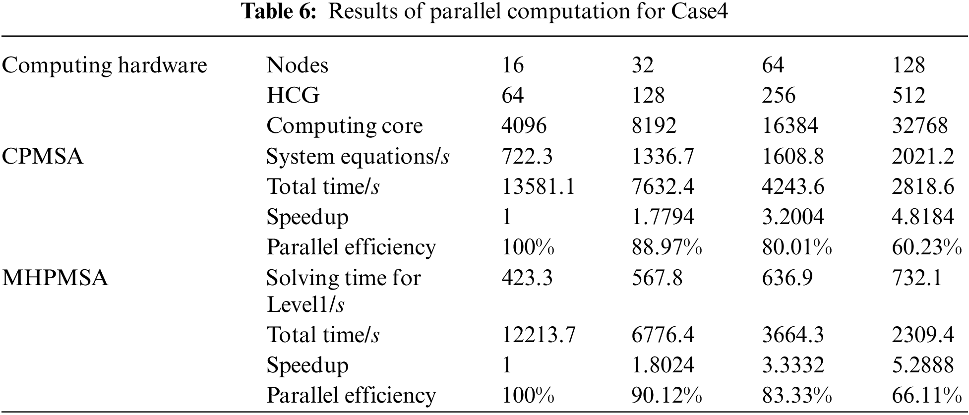
In Tables 4∼6, the total parallel computing time starts from calculating the subdomains and ends when the mode shape has been calculated for every subdomain. The solution time for level 1 subdomains includes: the time to form the equivalent stiffness matrix and the equivalent mass matrix of the level 1 subdomain, the time for condensation and reduction of the level 1 subdomain, the time for parallel solutions of the equations, and the time to back substitute level 1 subdomain modal coordinates. In Table 4, the global system equations are solved by parallel solvers SuperLU_D [35]. In Tables 5 and 6, the global system equations are solved by parallel PCG. Based on the results in Tables 4∼6, it can be observed that when using MHPMSA proposed in this article, we can obtain a higher acceleration ratio and parallel efficiency than using the CPMSA. This is because when using the CPMSA, with an increasing number of subdomains, the scale of GCEs and conditions also expands rapidly, resulting in a significant increase in solution time and thereby seriously affecting the overall parallel efficiency of the system. From a mathematical point of view, the MHPMSA method solution of the level 1 subdomain essentially solves the system’s GCEs with the same scale as the CPMSA and greatly shortens the solution time. For example, in Table 6, the solution time for the level 1 subdomain is 732.1 s with 512 computing cores, which saves 1289.1 s compared to the CPMSA. The main reason behind that is the MHPMSA, based on the two-level partitioning and four-transformation strategies, improves communication efficiency by separating the communication between inter-node and intra-node, together with the communication between HCGs and inside HCGs. Besides, it further reduces the system equation scale after condensation and accelerates its computation and iteration convergence rate. As a result, it can effectively save the solution time for the level 1 subdomain and obtain a satisfactory speedup ratio and parallel efficiency. Also, it can be observed that when using parallel PCG in the solving of global system equations, we can obtain a higher acceleration ratio and parallel efficiency, compared with SuperLU_D. This is because SuperLU_D will further increase the density of the original equations. As a consequence, the sets and triangular decomposition require a large amount of memory. Besides, it also needs a lot of communication and calculation.

The performance of the parallel algorithm for different test scales is shown in Fig. 11, according to Tables 5 and 6. It can be observed that the performance of the parallel algorithm of CPMSA and MHPMSA can be improved with the increase of the test scales. This is because the proportion of communication decreases with the increase of the test scales compared to the proportion of calculation. When the test scale is relatively large, MHPMSA can obtain a higher acceleration ratio and parallel efficiency than using the CPMSA. Hence, the proposed method showed good scalability with respect to the test scale.

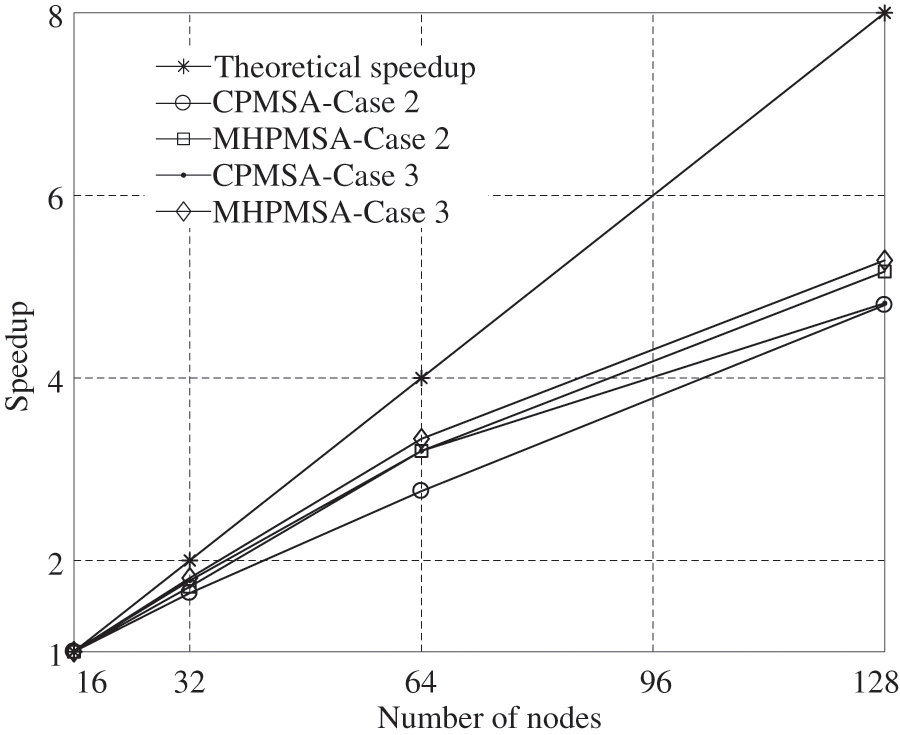
Figure 11: Performance of parallel algorithm for different test scale

4.2 A Typical Application of Cross-River Tunnel System

In real engineering applications, sometimes, complex engineering structures can contain multiple types of elements. In order to test the parallel efficiency of complex engineering systems under the scale of tens of millions of DOFs in multi-element hybrid modeling, a cross-river tunnel, as shown in Fig. 12, is taken as an example for analysis. This model has 2,896,781 solid elements, 186,121 beam elements, 21,685 mass elements, 1,012,581,369 non-zero elements of stiffness matrix, 412 average bandwidth and 13,167,203 DOFs. And we aim to solve its first 20 natural modal frequencies.

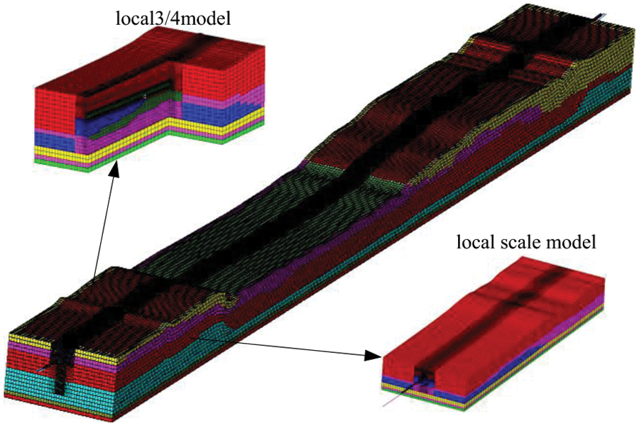
Figure 12: FEM of the cross-river tunnel structure system

In parallel computation, the total number of startup nodes is 32, 64, 128, and 256 in sequence with considering features of the ‘shenwei’ multicore processors and the storage of large-scale data. Each node starts using four HCGs during the test. And every HCG starts using one main core and 64 computing cores with 8 GB memory. The calculation results of the CPMSA and the MHPMSA proposed in this paper are shown in Table 7. The source of the original experimental data of Table 6 is the solution time, calculated by CPMSA and MHPMSA with different numbers of node machines. Then, the speedup and parallel efficiency can be calculated by Eqs. (13) and (14).

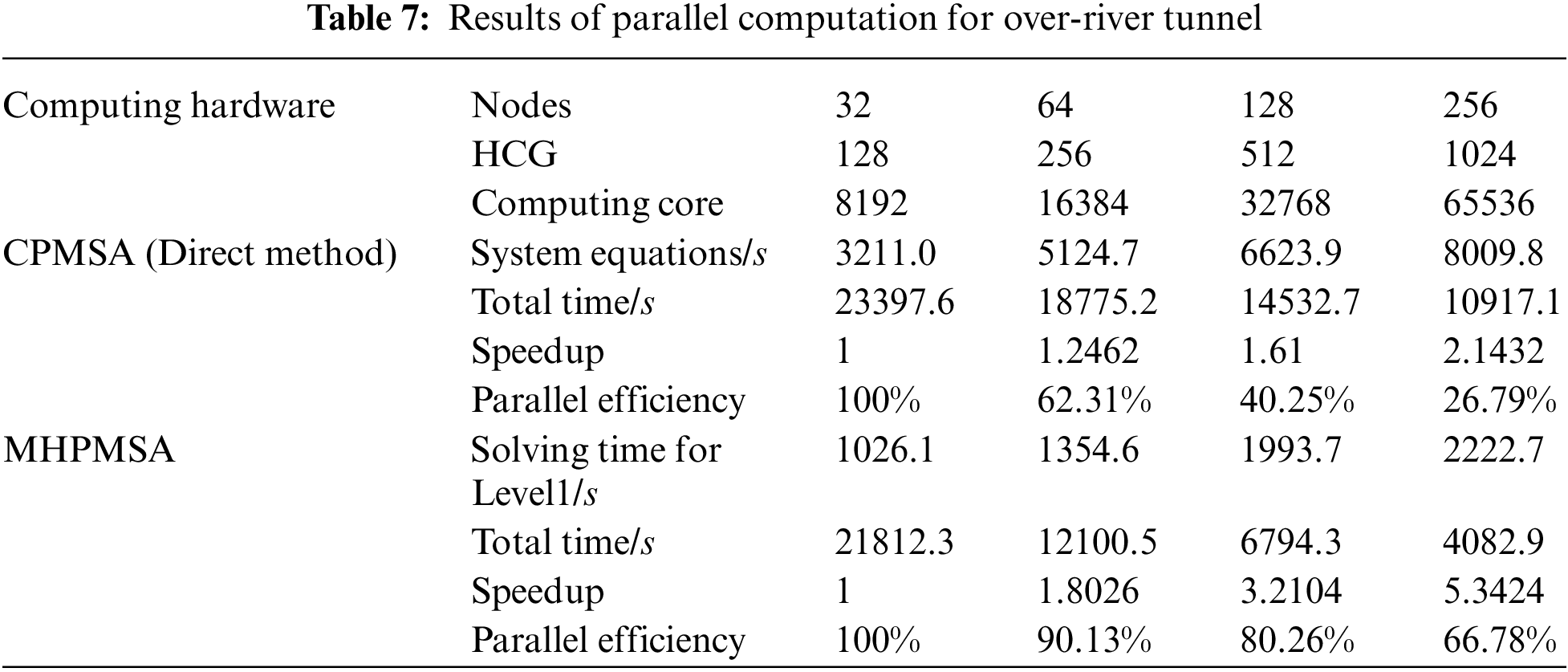
It can be seen from Table 7 that when using CPMSA to solve the overall system equations by the direct method, the solution time of the overall system equation increases sharply with the increase of subdomains, thus seriously reducing the parallel efficiency of the system. Although the overall system-level modal generalized characteristics adopt a compressed sparse column technique for storage, when conducting triangular decomposition, the PMCD is only applied in the lower triangle decomposition. The overall interface equation is still highly dense, and the triangular decomposition will further increase the density of the original equations. As a consequence, the sets and triangular decomposition require a large amount of memory. Besides, it also needs a lot of communication and calculation. With the increase of subdomain, the scale of the GCEs of the system after the overall reduction also gets larger. Companies with more expense in storage, communication and computing, and take a longer time for the overall solution of the system. On the contrary, when utilizing the MHPMSA, because of the use of the iterate method, there is no need to form the GCEs of the system after reduction. Moreover, the local communication involved in the equation parallel solution only exists between neighbour subdomains. As mentioned before, only a few dot product operations and computations for overall iterative errors need global communications. Thus, the proposed algorithm can achieve a better speedup ratio and parallel efficiency in a shorter computing time.

The calculation results of MHPMSA with different parallel solver on the solving of global GCEs are shown in Table 8.

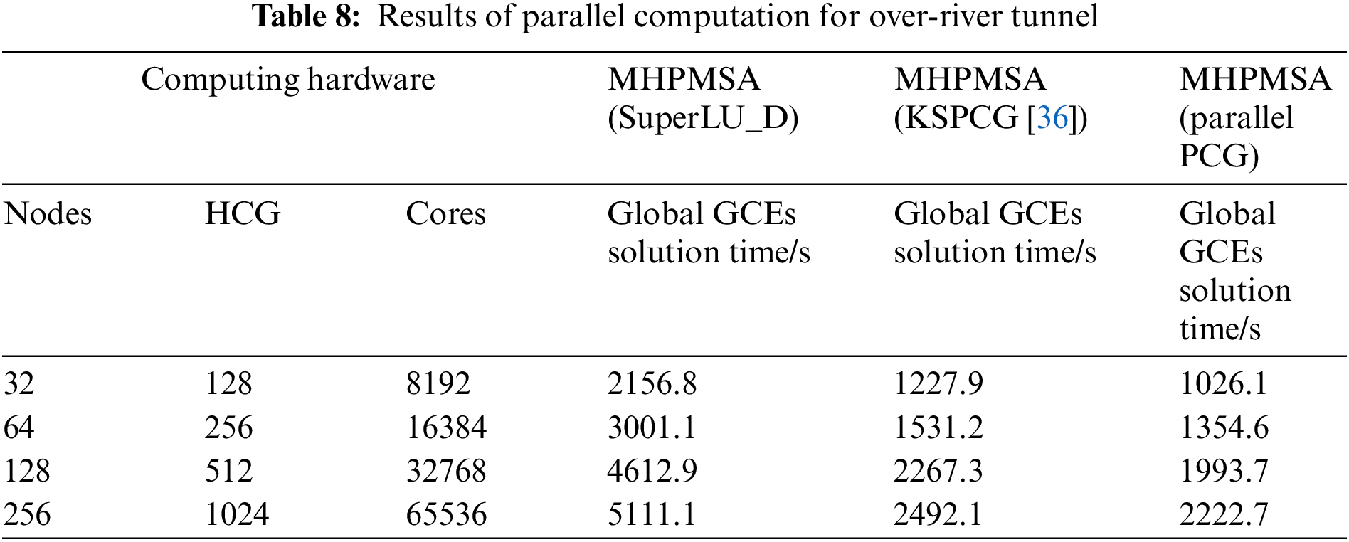
In Table 8, the global GCEs are solved by different parallel solvers SuperLU_D, KSPCG in PteSc and parallel PCG. It can be seen from the Table 8, the solution time of GCEs with KSPCG and parallel PCG can achieve the calculation in a shorter computing time, compared with SuperLU_D. This is because the local communication involved in the equation parallel solution only exists between neighbor subdomains during the calculation of global GCEs with KSPCG and paralle PCG. Only a few dot product operations and computations for overall iterative errors need global communications. Additionally, the solving time of KSPCG is more than parallel PCG. It is because only 1 MPI process within the node need to participate in global communication when solving global GCEs with parallel PCG. However, the KSPCG uses all MPI processes within the same node. Hence, the increment in inter-process communication and synchronization will greatly increase the solution time of global GCEs.

5  Conclusion

With the increase of the size and complexity of numerical simulation problems, heterogeneous supercomputers are becoming more and more popular in the high-performance computing field. However, it is still an open question how current applications can exploit the capabilities of parallel calculation with the best respect for the features of the architecture and execution mode of such heterogeneous systems. The main contribution of this paper is to provide a MHPMSA that is aware of the characteristics of ‘shenwei’ heterogeneous multicore processors and fully exploits their computing power to achieve optimal performance.

MHPMSA is on the basis of two-level partitioning and four transformation strategies. To match the features of ‘shenwei’ heterogeneous multicore processors, computing tasks of large-scale modal analysis are divided into 3 layers: inter-nodes, intra-nodes, HCGs, and inside HCGs. Through mapping computing tasks to different hardware layers of ‘shenwei’ heterogeneous multicore supercomputers can achieve load balancing among different layers and accomplish efficacious partitioning in communication. Then, MHPMSA not only realizes the sparsely distributed storage of a large amount of data and speeds up the access rate of data memory, but also reduces the scale of general GCEs after condensation effectively and saves the equation solution time. Finally, the typical numerical example shows that when compared with the CPMSA, the proposed method in this article can gain a higher speedup ratio and parallel efficiency. When under multiple work conditions, compared with the direct method of reduced GCEs of the whole system, this method can obtain a higher speedup ratio and parallel efficiency as well.

Although the authors’ current research only focuses on the large-scale modal analysis, MHPMSA is a general tool for solving many kinds of structural analysis problems, including linear dynamic analysis and nonlinear dynamic analysis, and so on. Hence, the research outcome of this paper can be provided as a reference for improving large-scale parallel computation efficiency and can be ported to other structural finite element analysis software for various analyses on Shenwei heterogeneous multicore processors or other heterogeneous multicore processors. It can also be used as a practical example and reference for large-scale equipment systems and complex engineering systems with finite modeling in parallel computation.

Acknowledgement: Not applicable.

Funding Statement: This work is supported by the National Natural Science Foundation of China (Grant No. 11772192).

Author Contributions: Gaoyuan Yu: Methodology, Software, Validation, Formal Analysis, Investigation, Writing-Original Draft. Yunfeng Lou: Methodology, Resources. Hang Dong: Writing-Review & Editing. Junjie Li: Methodology, Software. Xianlong Jin: Conceptualization, Supervision, Writing-Review & Editing.

Availability of Data and Materials: The raw data required to reproduce these findings cannot be shared at this time as the data also forms part of ongoing studies.

Conflicts of Interest: The authors declare that they have no conflicts of interest to report regarding the present study.

References

1. S. Xu, W. Wang, J. Zhang, J. R. Jiang, Z. Jin et al., “High performance computing algorithm and software for heterogeneous computing,” Journal of Software, vol. 32, no. 8, pp. 2365–2376, 2021. [Google Scholar]

2. R. Gao and X. Li, “Design and mechanical properties analysis of radially graded porous scaffolds,” Journal of Mechanical Engineering, vol. 57, no. 3, pp. 220–226, 2021. [Google Scholar]

3. G. K. Kennedy, G. J. Kennedy and J. R. Martins, “A parallel finite-element frameworks for large-scale gradient-based design optimization of high-performance structures,” Finite Elements in Analysis and Design, vol. 87, pp. 56–73, 2014. [Google Scholar]

4. P. H. Ni and S. S. Law, “Hybrid computational strategy for structural damage detection with short-term monitoring data,” Mechanical Systems and Signal Processing, vol. 70, pp. 650–663, 2016. [Google Scholar]

5. Y. Wang, Y. Gu and J. Liu, “A domain-decomposition generalized finite difference method for stress analysis in three-dimensional composite materials,” Applied Mathematics Letters, vol. 104, 106226, 2020. [Google Scholar]

6. M. Łoś, R. Schaefer and M. Paszyński, “Parallel space–time hp adaptive discretization scheme for parabolic problems,” Journal of Computational and Applied Mathematics, vol. 344, pp. 819–855, 2018. [Google Scholar]

7. X. Miao, X. Jin and J. Ding, “Improving the parallel efficiency of large-scale structural dynamic analysis using a hierarchical approach,” International Journal of High Performance Computing Applications, vol. 30, no. 2, pp. 156–168, 2016. [Google Scholar]

8. S. Zuo, Z. Lin, D. García-Doñoro, Y. Zhang and X. Zhao, “A parallel direct domain decomposition solver based on schur complement for electromagnetic finite element analysis,” IEEE Antennas and Wireless Propagation Letters, vol. 20, no. 4, pp. 458–462, 2021. [Google Scholar]

9. P. Tak, P. Tang and E. Polizzi, “Feast as a subspace iteration eigensolver accelerated by approximate spectral projection,” SIAM Journal on Matrix Analysis and Applications, vol. 35, no. 2, pp. 354–390, 2014. [Google Scholar]

10. S. Sundar and B. K. Bhagavan, “Generalized eigenvalue problems: Lanczos algorithm with a recursive partitioning method,” Computers & Mathematics with Applications, vol. 39, no. 7, pp. 211–224, 2000. [Google Scholar]

11. C. Duan and Z. Jia, “A global harmonic arnoldi method for large non-hermitian eigenproblems with an application to multiple eigenvalue problems,” Journal of Computational and Applied Mathematics, vol. 234, no. 3, pp. 845–860, 2010. [Google Scholar]

12. G. W. Stewart, “A Krylov-Schur algorithm for large eigenproblems,” SIAM Journal of Matrix Analysis and Applications, vol. 23, no. 3, pp. 601–614, 2002. [Google Scholar]

13. R. G. Grimes, J. G. Lewis and H. D. Simon, “A shifted block lanczos algorithm for solving sparse symmetric generalized eigenproblems,” SIAM Journal on Matrix Analysis and Applications, vol. 15, no. 1, pp. 228–272, 1996. [Google Scholar]

14. J. Yang, Z. Fu, Y. Zou, X. He, X. Wei et al., “A response reconstruction method based on empirical mode decomposition and modal synthesis method,” Mechanical Systems and Signal Processing, vol. 184, 109716, 2023. [Google Scholar]

15. B. Rong, K. Lu, X. Ni and J. Ge, “Hybrid finite element transfer matrix method and its parallel solution for fast calculation of large-scale structural eigenproblem,” Applied Mathematical Modeling, vol. 11, pp. 169–181, 2020. [Google Scholar]

16. B. C. P. Heng and R. I. Macke, “Parallel modal analysis with concurrent distributed objects,” Computers & Structures, vol. 88, no. 23–24, pp. 1444–1458, 2010. [Google Scholar]

17. Y. Aoyama and G. Yagawa, “Compoment mode synthesis for large-scale structural eigenanalysis,” Computers & Structures, vol. 79, no. 6, pp. 605–615, 2001. [Google Scholar]

18. P. Parik, J. G. Kim, M. Isoz and C. U. Ahn, “A parallel approach of the enhanced craig-bampton method,” Mathematics, vol. 9, no. 24, 3278, 2021. [Google Scholar]

19. J. Cui, J. Xing, X. Wang, Y. Wang, S. Zhu et al., “A simultaneous iterative scheme for the craig-bampton reduction based substructuring,” in Proc. Dynamics of Coupled Structures: Proc. of the 35 th IMAC, A Conf. and Exposition on Structural Dynamics, Garden Grove, CA, USA, vol. 4, pp. 103–114, 2017. [Google Scholar]

20. L. Gasparini, J. R. Rodrigues, D. A. Augusto, L. M. Carvalho, C. Conopoima et al., “Hybrid parallel iterative sparse linear solver framework for reservoir geomechanical and flow simulation,” Journal of Computational Science, vol. 51, 101330, 2021. [Google Scholar]

21. P. Ghysels and R. Synk, “High performance sparse multifrontal solvers on modern GPUs,” Parallel Computing, vol. 110, 102987, 2022. [Google Scholar]

22. J. Cui and G. Zheng, “An iterative state-space component modal synthesis approach for damped systems,” Mechanical Systems and Signal Processing, vol. 142, 106558, 2020. [Google Scholar]

23. C. U. Ahn, S. M. Kim, D. l. Park and J. G. Kim, “Refining characteristic constraint modes of component mode synthesis with residual modal flexibility,” Mechanical Systems and Signal Processing, vol. 178, 109265, 2022. [Google Scholar]

24. K. J. Bathe and J. Dong, “Component mode synthesis with subspace iterations for controlled accuracy of frequency and mode shape solutions,” Computers & Structures, vol. 139, pp. 28–32, 2014. [Google Scholar]

25. Q. Tian, Z. Yu, P. Lan, Y. Cui and N. Lu, “Model order reduction of thermo-mechanical coupling flexible multibody dynamics via free-interface component mode synthesis method,” Mechanism and Machine Theory, vol. 172, 104786, 2022. [Google Scholar]

26. C. D. Monjaraz Tec, J. Gross and M. Krack, “A massless boundary component mode synthesis method for elastodynamic contact problems,” Computers & Structures, vol. 260, 106698, 2022. [Google Scholar]

27. M. Warecka, G. Fotyga, P. Kowalczyk, R. Lech, M. Mrozowski et al., “Modal FEM analysis of ferrite resonant structures,” IEEE Microwave and Wireless Components Letters, vol. 32, no. 7, pp. 1–4, 2022. [Google Scholar]

28. Y. Aoyama and G. Yagawa, “Large-scale eigenvalue analysis of structures using component mode synthesis,” JSME International Journal. Series A, vol. 44, no. 4, pp. 631–640, 2001. [Google Scholar]

29. G. Karypis, K. Schloegel and V. Kumar, “ParMETIS-parallel graph partitioning and fill-reducting matrix ordering, version 4,” Department of Computer Science, University of Minnesota, 2014. [Online]. Available: http://glaros.dtc.umn.edu/gkhome/metis/parmetis/overview [Google Scholar]

30. M. Daga, A. M. Aji and W. Feng, “On the efficacy of a fused CPU+ GPU processor (or APU) for parallel computing,” in Proc. IEEE. Symp. on Application Accelerators in High-Performance Computing, Knoxville, TN, USA, pp. 141–149, 2011. [Google Scholar]

31. S. W. Keckler, W. J. Dally and B. Khailany, “GPUs and the future of parallel computing,” IEEE Micro, vol. 31, no. 5, pp. 7–17, 2011. [Google Scholar]

32. N. P. Carter, A. Agrawal and S. Borkar, “Runnemede: An architecture for ubiquitous high-performance computing,” in Proc. IEEE 19th Int. Symp. on High Performance Computer Architecture (HPCA), Shenzhen, China, pp. 198–209, 2013. [Google Scholar]

33. M. Hosseini Shirvani and R. Noorian Talouki, “Bi-objective scheduling algorithm for scientific workflows on cloud computing platform with makespan and monetary cost minimization approach,” Complex & Intelligent Systems, vol. 8, no. 2, pp. 1085–1114, 2022. [Google Scholar]

34. S. He, E. Jonsson and J. R. Martins, “Derivatives for eigenvalues and eigenvectors via analytic reverse algorithmic differentiation,” AIAA Journal, vol. 60, no. 4, pp. 2654–2667, 2022. [Google Scholar]

35. X. S. Li and J. W. Demmel, “SuperLU_DIST: A scalable distributed-memory sparse direct solver for unsymmetric linear systems,” ACM Transactions on Mathematical Software (TOMS), vol. 29, no. 2, pp. 110–140, 2003. [Google Scholar]

36. S. Balay, K. Buschelman, V. Eijkhout, W. D. Gropp, D. Kaushik et al., “PETSc users manual, ANL-95/11–Revision 3.17,” Argonne National Laboratory, 2022. [Google Scholar]