
 Submit a Paper
 Propose a Special lssue
 Open Access
ARTICLE

Stochastic Models to Mitigate Sparse Sensor Attacks in Continuous-Time Non-Linear Cyber-Physical Systems
1 Information Technologies Department, Universidad Politécnica de Madrid, Madrid, 28031, Spain
2 Geospatial Information Department, Universidad Politécnica de Madrid, Madrid, 28031, Spain
* Corresponding Author: Borja Bordel Sánchez. Email:
(This article belongs to the Special Issue: Advances in Information Security Application)
Computers, Materials & Continua 2023, 76(3), 3189-3218. https://doi.org/10.32604/cmc.2023.039466
Received 31 January 2023; Accepted 14 June 2023; Issue published 08 October 2023
 View Full Text
 Download PDF
Abstract
Cyber-Physical Systems are very vulnerable to sparse sensor attacks. But current protection mechanisms employ linear and deterministic models which cannot detect attacks precisely. Therefore, in this paper, we propose a new non-linear generalized model to describe Cyber-Physical Systems. This model includes unknown multivariable discrete and continuous-time functions and different multiplicative noises to represent the evolution of physical processes and random effects in the physical and computational worlds. Besides, the digitalization stage in hardware devices is represented too. Attackers and most critical sparse sensor attacks are described through a stochastic process. The reconstruction and protection mechanisms are based on a weighted stochastic model. Error probability in data samples is estimated through different indicators commonly employed in non-linear dynamics (such as the Fourier transform, first-return maps, or the probability density function). A decision algorithm calculates the final reconstructed value considering the previous error probability. An experimental validation based on simulation tools and real deployments is also carried out. Both, the new technology performance and scalability are studied. Results prove that the proposed solution protects Cyber-Physical Systems against up to 92% of attacks and perturbations, with a computational delay below 2.5 s. The proposed model shows a linear complexity, as recursive or iterative structures are not employed, just algebraic and probabilistic functions. In conclusion, the new model and reconstruction mechanism can protect successfully Cyber-Physical Systems against sparse sensor attacks, even in dense or pervasive deployments and scenarios.Keywords
Cyber-Physical Systems (CPS) are seamless integrations of physical and computational processes [1]. Many different architectures and approaches to support these unions have been reported, from schemes based on the control theory [2] to feedback loops in computational systems [3]. But all proposed CPS implementations include a sensing platform to monitor the evolution of the physical world [1]. That platform is dense, including thousands of networked sensor nodes capable of capturing information through several different physical parameters [4]. Those data must be injected into computational processes, to ensure that the cybernetic and physical worlds evolve together in a feedback control loop [5].
Therefore, precise information about physical processes is essential to ensure that the loop is convergent and follows the expected evolution [6]. However, it is hardly possible to obtain precise information in real applications [4]. Many random effects have an impact on the behavior of CPS, such as noise, transmission errors, measurement, digitalization, and discretization processes [4]. In that way, information finally injected into computational processes is not the raw or authentic information acquired from the physical world, but a non-deterministic transformation of it. And this transformed information prevents the CPS from integrating the computational and physical processes with the expected synchronicity and showing the required behavior [7].
Furthermore, as Cyber-Physical Systems are used in more scenarios and applications, including critical infrastructures, they are more exposed to new risks. Eventual and unexpected cyberattacks are the main ones. Although innovative attack strategies have been reported to exploit specific vulnerabilities of CPS [8], nowadays the greatest risks for CPS are still associated with classic cyberattacks such as the Sparse Sensor Attack (SSA). In the SSA [9], attackers introduce false information and/or cause delays in the sensing platform monitoring the physical world at a low level, so the CPS behavior is altered or denied. It is the most common attack in control solutions, and new uncertainty about the physical information injected into the computational processes is to be handled.
In this context, reconstruction mechanisms to recover the original and real information extracted from the physical world are essential [10]. The state of any CPS may be described as a multidimensional vector, where each position represents a physical parameter. By establishing the analytical law that describes the trajectory of all those state variables in the phase space, the transformed information received may be corrected through a theoretically predicted CPS state [11]. However, in the general case, all physical parameters are not independent, but they are interrelated through complex physical laws [12]. The appearance of complex non-linear laws, together with the need for stochastic terms to describe random effects such as sparse sensor cyberattacks, turns quite difficult to find a general high-precision model. Thus, traditional reconstruction schemes are based on some basic assumptions, so the mathematical expressions describing the evolution of CPS are easier to manipulate and implement [13].
Our work is motivated by limitations and vulnerabilities caused by these simple assumptions, which make CPS weaker against cyberattacks than other state-of-the-art technological systems. Namely:
• First, Cyber-Physical Systems are assumed to evolve according to a linear law.
• Second, all terms are considered deterministic, including noise and attacking signals.
• Third, all physical variables are assumed to be fully independent of each other.
• And fourth, physical processes are assumed to be discrete, so digitalization and transmission processes do not have to be explicitly considered. Although those linear deterministic models present important advantages (for example, they can be manipulated to find analytical expressions for the detection and identification of SSA), their applicability is very limited [14].
• Only closed CPS based on a reduced number of physical variables with a smooth and invariant behavior (such as the temperature in a climatized space) are governed and can be secured and protected by such a simple model.
Therefore, more complex and general models are required to protect and mitigate SSA in multidimensional CPS with a continuous-time non-linear behavior. In this paper, we address this challenge.
Three innovative contributions are introduced in this paper:
• A complex non-linear model to describe the CPS behavior in a general situation.
• New signals and models for SSA and digitalization processes.
• The third and final contribution is an innovative reconstruction scheme.
The proposed model describes the behavior of CPS using unknown generic functions, which are developed as Taylor series. This model also includes stochastic terms to represent physical, transmission, and measurement noises. Besides, SS attacks are described as a new signal whose value follows a probabilistic behavior according to a given discrete random variable. Physical processes are represented by continuous-time signals that are discretized using an event-based scheme. The resulting multidimensional model injects discrete data into computational processes, but is too complex to generate analytic expressions to mitigate SSA in CPS. Finally, the proposed reconstruction scheme is supported by a weighted stochastic model where the error probability is estimated through different indicators commonly employed to describe non-linear dynamics (such as the Fourier transform, first-return maps, or the probability density function). A decision algorithm calculates the final reconstructed value considering the previous error probability.
The rest of the paper is organized as follows. Section 2 analyzes the state-of-the-art on cyberattacks and countermeasures in CPS. Section 3 describes the proposed solution, including the mathematical model to describe the behavior of the CPS and the reconstruction and protection scheme to mitigate SSA. Finally, Section 4 describes the experimental validation and the results obtained. Section 5 concludes the paper.
Cyber-Physical Systems are one of the most promising technological revolutions nowadays. They are expected to govern all production, domestic, and critical digital systems. Due to this relevance, many authors have investigated how to protect CPS against various well-known and innovative attacks. In general, we can distinguish two different protection approaches: those based on control theory and those supported by Information Technologies (IT).
IT protection mechanisms for CPS are usually data processing and filtering modules to remove and correct malicious or corrupted data packets. Stochastic techniques and models [4], advanced filtering algorithms such as the Kalman filter [15], hardware-enabled algorithms such as parameter estimation [16], and pattern recognition techniques to identify unusual information [17] are the most common technologies. As well as game-theory and other common technologies for CPS protection, such as honeypots [18] or Software-Defined Networks [19]. However, a limited number of works supporting this vision may be found, as information theory techniques are high-level and agnostic concerning the underlying hardware platform [20]. And the most critical cyber risks in CPS nowadays are associated with sensor and actuator nodes [8]. Different authors have identified new attack vectors and strategies [8], so feedback loops in CPS can be used to magnify cyberattacks starting in a single hardware node and spreading throughout the entire system. Furthermore, these IT protection technologies are computationally heavy and require long processing times, so they are not effective against fast cyberattacks. Other low-level lightweight techniques are required.
Physical infrastructure protection is, then, a priority in CPS. And most works on CPS security employ control theory to design new hardware protection schemes. Globally, all these technologies follow the same strategy [21]: they estimate or predict a secure future state for the physical platform and/or control loop, which is used to mitigate different types of attacks. Although this paradigm could fully protect CPS [22], it is very difficult to implement in practice and the reported implementation presents different weaknesses. Techniques may be local (or decentralized), distributed, or centralized.
Decentralized state estimation techniques are handled by independent sensing nodes. They are sparse as individual sensors have very limited information and actuation capabilities, so the achieved protection level is poor. Continuous bidimensional linear models are employed to detect perturbations and attacks (typically Denial of Service attacks) and modify the behavior of nodes by, for example, increasing their computational resources [23]. The objective is to guarantee the local stability of the control loops by mitigating all perturbances [21]. In contrast, other decentralized CPS protection schemes use variance-based strategies (also known as ‘secure control’ [14]). This approach is more general and can be applied against a generic cyberattack. Using discrete bidimensional models, tuned filters and tuned control loops can be varied to reduce system errors, even while a cyberattack is running [24]. However, even if local control loops can operate normally, with variance-based techniques the global system is handling corrupted data, and that impacts the later global behavior. Some authors have shown that global system protection requires cooperation and information sharing among all agents [21]. Distributed techniques fill this gap.
Distributed secure state estimation is useful against systemic attacks such as Byzantine attacks [25]. System states are deducted through an optimization process where linear models represent the sensors’ outputs and graphs [26], Markov chains [27], binary decision trees [28], and other mathematical paradigms (such as the Lipschitz continuity) [29] are used to represent the interconnections and transmissions among nodes. Custom quasi-linear models for specific applications, such as series-parallel systems, have been also reported [30,31]. However, these protection mechanisms are passive and cannot deploy countermeasures to mitigate the impact of cyberattacks. Then, they must be complemented with specific controllers [32,33] to apply active protection policies on the CPS. Anyway, the final performance of distributed protection techniques is highly dependent on the number of trusted nodes, not affected by the attack [21,34]. Furthermore, linear and quasi-linear models cannot represent the output of most complex sensing platforms [35]. Thus, reported schemes can only be applied to a reduced number of application scenarios, excluding critical risks such as massive or viral attacks and common nonlinear algorithms.
On the other hand, recently distributed artificial intelligent solutions, such as federated learning [36], Support Vector Machines [37], feature selection [38] or eXplainable Artificial Intelligence (XAI) [39], have also been applied to CPS securitization and intrusion detection. But performance must be enhanced through additional techniques such as reinforcement learning [40]. Intelligent solutions must be designed for very specific attacks, as they are usually focused on Denial-of-Service attacks. Although the final results are promising, the balance between cost and performance is still worse than the one observed in other distributed techniques, and they are preferred to be used for privacy preservation [41].
The main disadvantage of distributed protection mechanisms is the increase in system congestion, due to the large number of transmissions required to run the distributed algorithms. On the contrary, centralized approaches may handle global stability and attacks (as distributed techniques) but with a lower system overload. Most reported works follow this paradigm.
Centralized control is usual in CPS, as it is the traditional approach in legacy Supervisory Control And Data Acquisition (SCADA) systems. Different kinds of multi-dimensional models are employed to represent the state of every single node on the platform. These models can be analytically manipulated to define protection algorithms based on Orthogonal-Triangular (QR) decomposition [42] or Linear–Quadratic (LQ) control [43], mitigating the impact of attacks. Models can be deterministic [44] or include some stochastic terms to represent noises [45]. Besides, continuous [44] and discrete [46] models may be found. However, most of these models are linear and only consider the self-maintained evolution of the node output and the measurement errors (in line with traditional control theory models). While other relevant effects, such as the digitalization process or the transmission protocols, are not considered, although they can be relevant. On the other hand, nonlinear models are very rare [47] and they are only developed for specific use cases. This centralized approach is successful against false information attacks (also known as sparse sensor attacks or deception attacks [14]), as it handles a full picture of the CPS. However, current models are very limited, and analytical protection algorithms have a reduced impact in real applications.
Table 1 summarizes the main current approaches and their associated open challenges.

In this paper, we address this challenge, with a continuous-time generic multidimensional non-linear model, and a protection policy based on probabilistic decision-making schemes.
The proposed solution includes two different phases. First, a multidimensional stochastic model is employed to estimate or predict the future state of the CPS. Later, the obtained secure state estimation is compared to the real state produced by the physical platform. Both values are compared using a probabilistic model, where several indicators are considered. The system state may be replaced or corrected using the predicted secure state if the decision-making algorithm indicates the information is false (corrupted or caused by an SSA). This section describes in detail the entire scheme. Section 3.1 introduces the stochastic model, while Section 3.2 presents the decision-making and protection algorithms.
3.1 Secure State Estimation. Model Description
A CPS is supported by a dense sensing platform including N different sensor nodes
Hereinafter we are naming
The information to be finally injected into the computational processes (or system state) is a set of M discrete state variables
The physical world (i) is considered a closed autonomous system, with no external intervention, so the future evolution of the physical variables is only determined by the past values of those same variables (5). The function relating the past and future values of the physical variables
Any multidimensional function may be developed as Taylor’s series using the partial derivation (7). For simplicity, we are using a McLaurin development around the origin. In this expression terms
The second process represented by the system function
Unknown function
Although white noises
Finally, it is necessary to estimate the value for mean
The transduction phase is open, so it can be affected by SSA and malicious signals. In order to represent this risk, we are considering a set of additive malicious signals
Finally, as every sensor node
The third subprocess to be represented in our model is the measurement scheme (iii). This, basically, is a digitalization scheme, developed internally by sensor nodes (see Fig. 1). Discrete signal

Figure 1: Ideal sampling scheme
In this digitalization process only the quantification noise
where
The fourth process to be represented is the data transmission (iv). In general, hardware platforms in CPS are low-energy, and they sleep most of the time. Being event-based, they only activate the transmission subsystem when an event is detected in the physical world. We are defining function
Data transmission is, once again, an open process, so it is vulnerable to attacks. Denial-of-Service (DoS) attacks in this case. But SSA too (as the transduction phase). Bernoulli distribution
All parameters and their meaning are equivalent to distributions
In our model, a DoS attack is represented by an arbitrary delay of
Our model considers
Finally, information injected into computational processes
Function
Then, the final analytical model to describe the behavior of CPS includes five different Eq. (40). All parameters and coefficients are known (or may be estimated) but
3.2 Reconstruction and Protection Mechanisms
The proposed model (see Section 3.1) considers seven sources of perturbations. On the one hand, errors may be caused by four different phenomena: erratic behaviors in the physical variables, electrical noises, quantification noise, and transmission perturbations. And, on the other hand, three different potential attacks affect CPS in the general case: SSA at the transduction phase, and SSA and Denial-of-Service attacks at the transmission phase. Fig. 2 represents the proposed reconstruction and protection mechanisms.
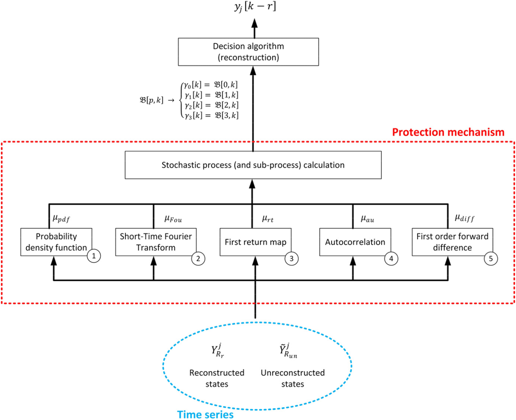
Figure 2: Protection and reconstruction mechanism
As a novelty, the proposed reconstruction and protection mechanism evaluates all these potential perturbations to build a global stochastic process (contrary to traditional deterministic models). This stochastic process
In the proposed protection mechanism, five indicators are employed to evaluate the probability distribution of the stochastic process
In order to make feasible the calculation of all these indicators from time series
Regarding the probability density function ①, the probability
But even if the unreconstructed CPS state has a relevant probability, it can still be manipulated and not be coherent with the system evolution. This situation may be detected through two different indicators: the Short-Time Fourier Transform (STFT) and the first-return map. Considering the Short-Time Fourier Transform (STFT) ②, the Fourier spectrum tends to be stable in a CPS, so any abrupt change may indicate an attack. The STFT (47) is equivalent to the traditional Fourier transform, but only considering a limited number of samples (instead of the usual infinite sum) through a window function
Then, using the Euclidean definition for distance, we can analyze how different
Another indicator we can use to identify situations where the unreconstructed CPS state is manipulated is the first-return map ③. The first return map is a function
But in some situations, very noisy states are difficult to distinguish from attacks. To clarify and separate these two situations we use the autocorrelation ④. Noise is a random effect, so autocorrelation tend to the null value very quickly. While planned attacks follow a certain structure, and autocorrelation oscillates but not disappears because of these patterns. But autocorrelation cannot be directly applied to series

Figure 3: Stop-band filtering for autocorrelation calculation
From the STFT
This autocorrelation
However, some attacks may use perturbations within the information signals’ bandwidth, and autocorrelation may not generate a conclusive result. To analyze this situation, we are using our last indicator, the first order forward difference ⑤. The first order forward difference
Using these five indicators, we can now estimate the probability distribution of the stochastic process
Being
On the other hand, SSA-attacked state (
Being
In an equivalent manner we may calculate the probability distribution for all stochastic subprocesses
Based on this stochastic process
Fig. 4 shows the proposed decision algorithm. This is an original contribution firstly presented in this work. In the first step it is evaluated if any global probability

Figure 4: Reconstruction and protection algorithm
If no global probability
If no probability
Sizes for parameters
To validate the proposed mechanisms for the protection of Cyber-Physical Systems against Sparse Sensor and Denial of Service attacks, an experimental validation was conducted. Section 4.1 describes the experimental methodology, while Section 4.2 presents the obtained results.
4.1 Experimental Methodology and Environment
The experiments were based on an emulated industrial scenario with real hardware devices (microcontrollers). The experimental works were divided into two different phases. First, we focused on analyzing the precision and attack detection capacity of the proposed technology. The second phase focused on studying the performance and scalability of the proposed model and the reconstruction and protection mechanism.
For all the experiments, the proposed CPS was supported by a collection of ESP-32 microcontrollers. Its number is variable depending on the experiment. ESP-32 microcontrollers are low-cost System-on-Chip provided with Wireless Fidelity (WiFi) and Bluetooth capabilities. It is based on a Tensilica Xtensa LX6 processor, and it includes several peripheral interfaces (Universal Asynchronous Receiver-Transmitter-UART-, Pulse Width Modulation-PWM-, Serial Peripheral Interface-SPI-, etc.), so it can handle a large catalog of different sensors. In our experiments, each ESP-32 node was provided with two sensors, monitoring four physical variables in total. The first sensor was a CCS811 sensor to monitor air quality. It can provide two different variables: carbon dioxide equivalent (eCO2) and organic volatile compounds concentration (TVOC). The second sensor is a DTH-11 device, which generates measurements for the environmental humidity and temperature. The measurement periodicity is variable and depends on the experiment.
All these sensors employed a WiFi connection to send all the collected information to a cloud server, located within the same building. Hypertext Transfer Protocol (HTTP) messages and Representational State Transfer (REST) interfaces were employed to support these communications. The server was a Linux-based machine (Ubuntu 18.04 LTS) with the following hardware characteristics: Dell R540 Rack 2U, 96 GB RAM, two processors Intel Xeon Silver 4114 2.2G, HD 2 TB SATA 7,2K rpm. In this server, both the proposed model and the reconstruction and protection algorithm were hosted and executed. A Node.js server was deployed to collect all data from the sensor nodes and send them to the computational process executing our proposal. A supervisory process was continuously evaluating the evolution and performance of the proposed algorithms and model. The acquired information was employed to carry out a statistical analysis using the MATLAB 2022a software, to validate our hypotheses. All experiments were repeated twelve times to remove possible spurious effects. The results for every measurement are obtained as the average of all these individual twelve realizations.
In the first phase, we performed two different experiments. The first experiment was aimed at analyzing the precision of the proposed model (Section 3.1) by comparing (using the Mean Square Error metric) the information received by the computational processes in the real CPS deployment and the samples predicted by the proposed model. Data were collected for 24 h, and the relative (percentage) Mean Square Error was calculated for all the acquired samples. The experiment was repeated for different values of parameters
The second experiment in this first phase was aimed at analyzing the probability of the proposed reconstruction and protection algorithm to successfully detect the real situation that occurs in the CPS. Some additional ESP32 nodes were deployed to increment the electrical noise in the environment and/or perform Sparse Sensor and Denial of Service attacks. Different situations were generated, with a duration of ten minutes. It was monitored if the proposed algorithm was able to identify them properly. The second experiment had a duration of 24 h too. Results were processed to generate a confusion matrix representing the algorithm’s behavior. The experiment was repeated for different values of
In the second experimental phase, we evaluated the performance and scalability. We measured the computational time needed for the proposed model and the reconstruction and protection algorithm to obtain a final and stable output. The first experiment focused on the mathematical model. The calculation time was analyzed for different values of parameters
Finally, the second experiment in this second phase evaluated the computational time required by the reconstruction and protection algorithm. The experiment was repeated for different values of
To evaluate the behavior of the proposed technology, first, we analyze the precision of our model (Section 3.1), comparing the predicted future CPS states and the actual state finally achieved. Fig. 5 shows the results. As can be seen, the evolution is exponential, as expected from the error in the Taylor series, as the number of terms increases. In general, all configurations show good behavior, although models with only two terms introduce an error of 12% (which may be too high for some applications). The minimum error (2%) may be achieved for models with more than 12 terms. This error is caused by the truncation of the Taylor series, so they can be numerically computed. But, as a counterpart, the resulting finite series does not perfectly represent the original function and we are introducing a numerical error.
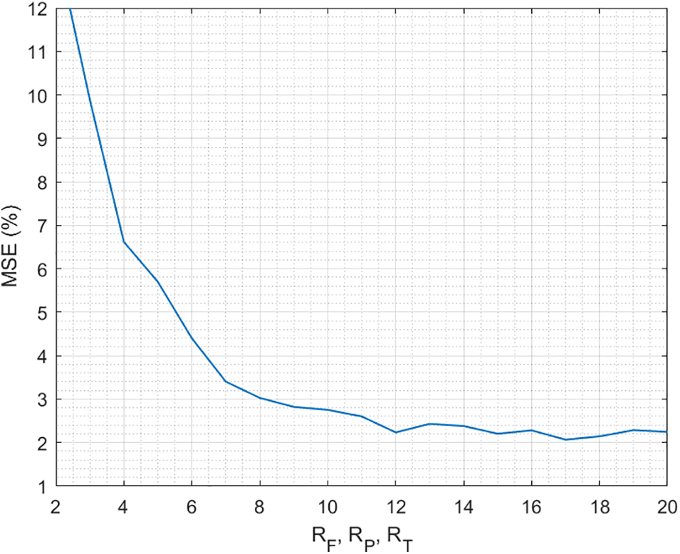
Figure 5: Precision of the proposed model
Other limitations in the proposed model (such as the numerical precision of the underlying hardware platform) are also affecting, so, only by increasing the number of terms in Taylor’s series cannot reduce the global error as much as desired. But for a very large catalog of applications, an error of 2% is acceptable and can be tolerated. Even, for those scenarios where computationally lightweight solutions are preferred, schemes with four or five terms generate an error of around 6%, which is a standard error for mass non-critical applications. In common applications, errors below 10% can be handled. From these results, we can conclude that the proposed model represents with good precision the physical processes in CPS.
Similarly, we need to analyze the capacity of the proposed reconstruction algorithm to successfully detect the real situation that is happening in the CPS. Fig. 6 shows the results of this experiment. For all possible situations, three regions are identified. First, for low values of
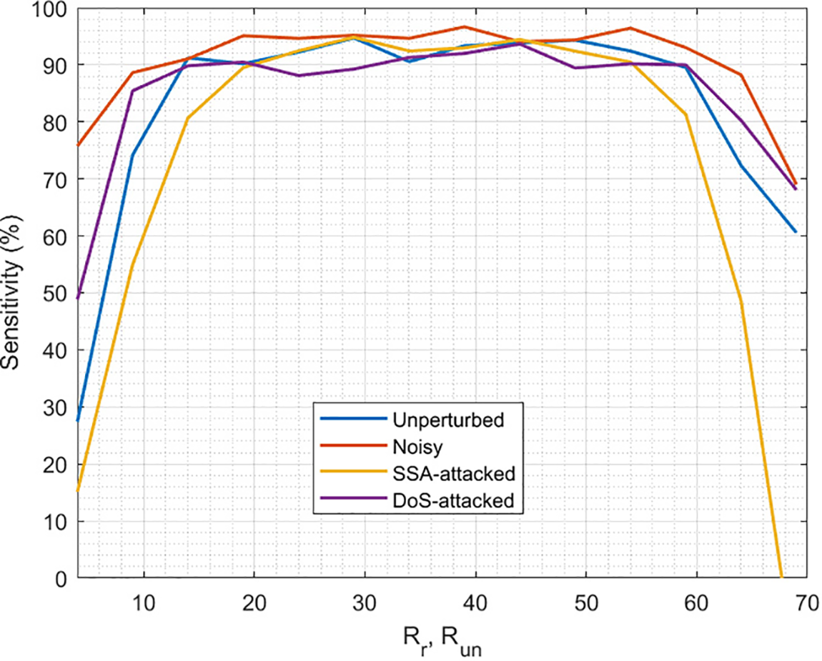
Figure 6: Precision of the proposed reconstruction and protection
In conclusion,
On the other hand, the proposed algorithm does not show the same sensitivity when detecting the different situations in a CPS. In general, situations whose probability is calculated using functions with a higher growth rate (such as the exponential) are more sensitive to the quality of indicators representing the CPS (first return maps, STFT, etc.) and then more sensible to the value of
Anyway, the sensitivity of the proposed algorithm (in balanced values of
To go deeper into the analysis of these data, we present the complete confusion matrix (Table 2) for the configuration

As can be seen, most errors when identifying the situation in the CPS are false detections of the noisy situation. Probably, that is caused by the linear term in its probability function, which does not reduce its value as much as the exponential function. If this sensitivity needs to be improved, that linear term should be enriched with new indicators and functions.
It is also important to evaluate the performance and scalability of the proposed solution to identify its limitations. Fig. 7 shows the computational time required for the proposed model to operate.

Figure 7: Computational delay and scalability (mathematical model)
As can be seen, the evolution of the computational delay is linear. This is because our model consists of additions and multiplications, without loops or recursive problems. Besides, each new state variable is independent of the others, so the increase is linear. This facilitates the employment of this protection and reconstruction solution in future dense and pervasive scenarios, where up to ten million sensors per square kilometer could be deployed.
Moreover, the delay is always in the range of milliseconds. Additions and multiplications are performed very efficiently on modern computers, and they require a short time to perform millions of operations. In this case, even for a CPS that includes 100 devices (i.e., 400 state variables) and very complex models (with almost 20 terms in the Taylor series), the computational time required to operate the model is below 100 milliseconds (70 milliseconds, to be precise). Considering the most usual Cyber-Physical Systems capture information from the environment every few seconds, this delay is satisfactory.
Finally, the same scalability and performance analysis must be applied to the reconstruction and protection algorithm. Fig. 8 shows the results. Here, again, the evolution is almost linear, because all the proposed computational procedures do not require any loop or recursive processing. In this case, for the largest deployment (one hundred devices) and a typical value for

Figure 8: Computational delay and scalability (reconstruction and protection algorithm)
In conclusion, considering the limitations that may arise in critical real-time applications, the performance of the proposed reconstruction and protection mechanism is satisfactory.
5 Conclusions and Future Works
This paper presents a new stochastic model to represent the behavior of Cyber-Physical Systems precisely. This model includes unknown multivariate discrete and continuous-time functions and different multiplicative noises to represent the evolution of physical processes and random effects in the physical and computational worlds. As a novelty, in this model, engineered processes such as the digitalization stage are represented too. Additionally, and contrary to the commonly employed deterministic attackers, in this new model attackers are described through a stochastic process. Standard error sources are estimated through different indicators and non-linear techniques (such as the Fourier transform, first-return maps, or the probability density function). Finally, the reconstruction mechanism consists of a weighted stochastic model combining all error sources. The actual reconstructed value is generated as the output from a decision algorithm.
Experimental results show that the precision of the proposed model is above 90%, with a residual error between 6% and 2% for the most common configurations. Additionally, the sensitivity of the proposed reconstruction and protection algorithm is up to 92%. Considering all this, the proposed solution is a valid security scheme for CPS.
Future works will analyze new indicators and probability functions to improve the sensitivity, especially in noisy situation. In addition, the solution will be deployed in real industrial scenarios with legacy systems, to study the impact of second-order effects such as reduced connectivity or human accidents and manipulations.
Acknowledgement: The authors also gratefully acknowledge the helpful comments and suggestions of the reviewers, which have improved the presentation.
Funding Statement: This work is supported by Comunidad de Madrid within the framework of the Multiannual Agreement with Universidad Politécnica de Madrid to encourage research by young doctors (PRINCE).
Author Contributions: The authors confirm contribution to the paper as follows: study conception and design: Borja Bordel; data collection: Ramón Alcarria, Borja Bordel; analysis and interpretation of results: Ramón Alcarria, Tomás Robles; draft manuscript preparation: Borja Bordel, Tomás Robles. All authors reviewed the results and approved the final version of the manuscript.
Availability of Data and Materials: Data sharing is not applicable to this article as no new data were created or analyzed in this study.
Conflicts of Interest: The authors declare that they have no conflicts of interest to report regarding the present study.
References
1. S. Zanero, “Cyber-physical systems,” Computer, vol. 50, no. 4, pp. 14–16, 2017. [Google Scholar]
2. S. Yin, J. J. Rodriguez-Andina and Y. Jiang, “Real-time monitoring and control of industrial cyberphysical systems: With integrated plant-wide monitoring and control framework,” IEEE Industrial Electronics Magazine, vol. 13, no. 4, pp. 38–47, 2019. [Google Scholar]
3. F. C. Delicato, A. Al-Anbuky, I. Kevin and K. Wang, “Smart cyber–physical systems: Toward pervasive intelligence systems,” Future Generation Computer Systems, vol. 107, pp. 1134–1139, 2020. [Google Scholar]
4. B. Bordel, R. Alcarria, T. Robles and A. Sánchez-Picot, “Stochastic and information theory techniques to reduce large datasets and detect cyberattacks in ambient intelligence environments,” IEEE Access, vol. 6, pp. 34896–34910, 2018. [Google Scholar]
5. E. A. Lee, “Cyber-physical systems-are computing foundations adequate,” Position Paper for NSF Workshop on Cyber-Physical Systems: Research Motivation, Techniques and Roadmap, vol. 2, pp. 1–9, 2006. [Google Scholar]
6. N. Negi and A. Chakrabortty, “Co-design of delays and sparse controllers for bandwidth-constrained cyber-physical systems,” in 2020 American Control Conf. (ACC), Denver, CO, USA, IEEE, pp. 987–992, 2020. [Google Scholar]
7. N. Wang and X. Li, “Secure synchronization control for a class of cyber-physical systems with unknown dynamics,” IEEE/CAA Journal of Automatica Sinica, vol. 7, no. 5, pp. 1215–1224, 2020. [Google Scholar]
8. V. Bolbot, G. Theotokatos, L. M. Bujorianu, E. Boulougouris and D. Vassalos, “Vulnerabilities and safety assurance methods in cyber-physical systems: A comprehensive review,” Reliability Engineering & System Safety, vol. 182, pp. 179–193, 2019. [Google Scholar]
9. Y. Shoukry and P. Tabuada, “Event-triggered state observers for sparse sensor noise/attacks,” IEEE Transactions on Automatic Control, vol. 61, no. 8, pp. 2079–2091, 2015. [Google Scholar]
10. H. Wang, X. Wen, Y. Xu, B. Zhou, J. Peng et al., “Operating state reconstruction in cyber physical smart grid for automatic attack filtering,” IEEE Transactions on Industrial Informatics, vol. 18, no. 5, pp. 2909–2922, 2020. [Google Scholar]
11. M. Al-Sharman, D. Murdoch, D. Cao, C. Lv, Y. Zweiri et al., “A sensorless state estimation for a safety-oriented cyber-physical system in urban driving: Deep learning approach,” IEEE/CAA Journal of Automatica Sinica, vol. 8, no. 1, pp. 169–178, 2020. [Google Scholar]
12. A. Akbarzadeh, P. Pandey and S. Katsikas, “Cyber-physical interdependencies in power plant systems: A review of cyber security risks,” in 2019 IEEE Conf. on Information and Communication Technology (CICT), Allahabad, India, IEEE, pp. 1–6, 2019. [Google Scholar]
13. H. Yang, S. Yin, H. Han and H. Sun, “Sparse actuator and sensor attacks reconstruction for linear cyber-physical systems with sliding mode observer,” IEEE Transactions on Industrial Informatics, vol. 18, no. 6, pp. 3873–3884, 2021. [Google Scholar]
14. D. Zhang, Q. G. Wang, G. Feng, Y. Shi and A. V. Vasilakos, “A survey on attack detection, estimation and control of industrial cyber–physical systems,” ISA Transactions, vol. 116, pp. 1–16, 2021. [Google Scholar] [PubMed]
15. H. Karimipour and H. Leung, “Relaxation-based anomaly detection in cyber-physical systems using ensemble kalman filter,” IET Cyber-Physical Systems: Theory & Applications, vol. 5, no. 1, pp. 49–58, 2020. [Google Scholar]
16. T. D. Memon, “FPGA implementation of extended kalman filter for parameters estimation of railway wheelset,” Computers, Materials & Continua, vol. 74, no. 2, pp. 3351–3370, 2022. [Google Scholar]
17. Z. Lv, D. Chen, R. Lou and A. Alazab, “Artificial intelligence for securing industrial-based cyber–physical systems,” Future Generation Computer Systems, vol. 117, pp. 291–298, 2021. [Google Scholar]
18. M. S. Miah, M. Zhu, A. Granados, N. Sharmin, I. Anjum et al., “Optimizing honey traffic using game theory and adversarial learning,” in Cyber Deception: Techniques, Strategies, and Human Aspects. Cham: Springer, pp. 97–124, 2022. [Google Scholar]
19. A. Wani and R. Khaliq, “SDN-based intrusion detection system for IoT using deep learning classifier (IDSIoT-SDL),” CAAI Transactions on Intelligence Technology, vol. 6, no. 3, pp. 281–290, 2021. [Google Scholar]
20. J. P. A. Yaacoub, O. Salman, H. N. Noura, N. Kaaniche, A. Chehab et al., “Cyber-physical systems security: Limitations, issues and future trends,” Microprocessors and Microsystems, vol. 77, pp. 103201–103234, 2020. [Google Scholar] [PubMed]
21. D. Ding, Q. L. Han, X. Ge and J. Wang, “Secure state estimation and control of cyber-physical systems: A survey,” IEEE Transactions on Systems, Man, and Cybernetics: Systems, vol. 51, no. 1, pp. 176–190, 2020. [Google Scholar]
22. H. Fawzi, P. Tabuada and S. Diggavi, “Secure estimation and control for cyber-physical systems under adversarial attacks,” IEEE Transactions on Automatic Control, vol. 59, no. 6, pp. 1454–1467, 2014. [Google Scholar]
23. A. Y. Lu and G. H. Yang, “Observer-based control for cyber-physical systems under denial-of-service with a decentralized event-triggered scheme,” IEEE Transactions on Cybernetics, vol. 50, no. 12, pp. 4886–4895, 2019. [Google Scholar]
24. L. Ma, Z. Wang, Q. L. Han and H. K. Lam, “Variance-constrained distributed filtering for time-varying systems with multiplicative noises and deception attacks over sensor networks,” IEEE Sensors Journal, vol. 17, no. 7, pp. 2279–2288, 2017. [Google Scholar]
25. M. S. Mahmoud, M. M. Hamdan and U. A. Baroudi, “Modeling and control of cyber-physical systems subject to cyber attacks: A survey of recent advances and challenges,” Neurocomputing, vol. 338, pp. 101–115, 2019. [Google Scholar]
26. L. An and G. H. Yang, “Distributed secure state estimation for cyber–physical systems under sensor attacks,” Automatica, vol. 107, pp. 526–538, 2019. [Google Scholar]
27. X. Xie, Z. Yang and X. Mu, “Observer-based consensus control of nonlinear multiagent systems under semi-Markovian switching topologies and cyber attacks,” International Journal of Robust and Nonlinear Control, vol. 30, no. 14, pp. 5510–5528, 2020. [Google Scholar]
28. V. S. Gaur, V. Sharma and J. McAllister, “Abusive adversarial agents and attack strategies in cyber-physical systems,” CAAI Transactions on Intelligence Technology, vol. 8, no. 1, pp. 149–165, 2023. [Google Scholar]
29. W. He, Z. Mo, Q. L. Han and F. Qian, “Secure impulsive synchronization in Lipschitz-type multi-agent systems subject to deception attacks,” IEEE/CAA Journal of Automatica Sinica, vol. 7, no. 5, pp. 1326–1334, 2020. [Google Scholar]
30. M. U. Danjuma, B. Yusuf and I. Yusuf, “Reliability, availability, maintainability, and dependability analysis of cold standby series-parallel system,” Journal of Computational and Cognitive Engineering, vol. 1, no. 4, pp. 193–200, 2022. [Google Scholar]
31. A. S. Maihulla, I. Yusuf and S. I. Bala, “Reliability and performance analysis of a series-parallel system using Gumbel–Hougaard family copula,” Journal of Computational and Cognitive Engineering, vol. 1, no. 2, pp. 74–82, 2022. [Google Scholar]
32. H. Modares, B. Kiumarsi, F. L. Lewis, F. Ferrese and A. Davoudi, “Resilient and robust synchronization of multiagent systems under attacks on sensors and actuators,” IEEE Transactions on Cybernetics, vol. 50, no. 3, pp. 1240–1250, 2019. [Google Scholar] [PubMed]
33. R. Moghadam and H. Modares, “Resilient autonomous control of distributed multiagent systems in contested environments,” IEEE Transactions on Cybernetics, vol. 49, no. 11, pp. 3957–3967, 2018. [Google Scholar] [PubMed]
34. B. Bordel, R. Alcarria, D. Martín and D. Sánchez-de-Rivera, “An agent-based method for trust graph calculation in resource constrained environments,” Integrated Computer-Aided Engineering, vol. 27, no. 1, pp. 37–56, 2020. [Google Scholar]
35. L. Zhang, X. Chen, F. Kong and A. A. Cardenas, “Real-time attack-recovery for cyber-physical systems using linear approximations,” in 2020 IEEE Real-Time Systems Symp. (RTSS), Houston, TX, USA, IEEE, pp. 205–217, 2020. [Google Scholar]
36. Z. Guo, K. Yu, Z. Lv, K. K. R. Choo, P. Shi et al., “Deep federated learning enhanced secure POI microservices for cyber-physical systems,” IEEE Wireless Communications, vol. 29, no. 2, pp. 22–29, 2022. [Google Scholar]
37. A. Chakraborty, M. Alam, V. Dey, A. Chattopadhyay and D. Mukhopadhyay, “A survey on adversarial attacks and defences,” CAAI Transactions on Intelligence Technology, vol. 6, no. 1, pp. 25–45, 2021. [Google Scholar]
38. I. Hidayat, M. Z. Ali and A. Arshad, “Machine learning-based intrusion detection system: An experimental comparison,” Journal of Computational and Cognitive Engineering, vol. 2, pp. 88–97, 2022. [Google Scholar]
39. B. A. Alqaralleh, F. Aldhaban, E. A. AlQarallehs and A. H. Al-Omari, “Optimal machine learning enabled intrusion detection in cyber-physical system environment,” Computers, Materials & Continua, vol. 72, no. 3, pp. 4691–4707, 2022. [Google Scholar]
40. P. Dai, W. Yu, H. Wang, G. Wen and Y. Lv, “Distributed reinforcement learning for cyber-physical system with multiple remote state estimation under DoS attacker,” IEEE Transactions on Network Science and Engineering, vol. 7, no. 4, pp. 3212–3222, 2020. [Google Scholar]
41. Y. Lu, X. Huang, Y. Dai, S. Maharjan and Y. Zhang, “Federated learning for data privacy preservation in vehicular cyber-physical systems,” IEEE Network, vol. 34, no. 3, pp. 50–56, 2020. [Google Scholar]
42. J. Zhou, B. Chen, T. Li and L. Yu, “Secure estimation against non-fixed channel attacks in cyber-physical systems,” International Journal of Robust and Nonlinear Control, vol. 33, no. 3, pp. 2496–2507, 2023. [Google Scholar]
43. L. Zhang, Y. Chen and M. Li, “Resilient predictive control for cyber–physical systems under denial-of-service attacks,” IEEE Transactions on Circuits and Systems II: Express Briefs, vol. 69, no. 1, pp. 144–148, 2021. [Google Scholar]
44. M. Zhang and C. Lin, “Secure state estimation for cyber physical systems with state delay and sparse sensor attacks,” Systems Science & Control Engineering, vol. 9, pp. 71–80, 2021. [Google Scholar]
45. A. Y. Lu and G. H. Yang, “Detection and identification of sparse sensor attacks in cyber physical systems with side information,” IEEE Transactions on Automatic Control, vol. 2022, pp. 1–15, 2022. [Google Scholar]
46. D. Ding, Z. Wang, G. Wei and F. E. Alsaadi, “Event-based security control for discrete-time stochastic systems,” IET Control Theory & Applications, vol. 10, no. 15, pp. 1808–1815, 2016. [Google Scholar]
47. S. Nateghi, Y. Shtessel, R. J. Rajesh and S. S. Das, “Control of nonlinear cyber-physical systems under attack using higher order sliding mode observer,” in 2020 IEEE Conf. on Control Technology and Applications (CCTA), Montreal, Canada, IEEE, pp. 1–6, 2020. [Google Scholar]
Cite This Article
 Copyright © 2023 The Author(s). Published by Tech Science Press.
This work is licensed under a Creative Commons Attribution 4.0 International License , which permits unrestricted use, distribution, and reproduction in any medium, provided the original work is properly cited.
 Downloads
 Citation Tools