Automatic Aggregation Enhanced Affinity Propagation Clustering Based on Mutually Exclusive Exemplar Processing

1  Introduction

In the field of unsupervised learning, cluster analysis is a crucial technology. It aims at separating elements into distinct categories based on certain similarity assessment criteria and result evaluation indexes. Elements with high similarity are commonly classified into the same cluster, whereas elements in different clusters have lower similarity. With the fast development of information technology, clustering is required to address realistic challenges in numerous technical fields, including image segmentation, text mining, network analysis, target recognition, trajectory analysis, and gene analysis, which in turn enhance the continuous development of clustering approaches [1–4].

The existing clustering approaches can be generally divided into subsequent categories. The partitioning-based approach usually assumes that the data set must be classified into K clusters, and iteratively searches for the optimal centers and data partitioning through certain criteria. The benefits are comprehensible, but usually, there is a dearth of prior knowledge about the number of clusters. The representative approaches are K-means [5], K-medoids [6], and Fuzzy C-means (FCM) [7]. Hierarchical clustering approaches mainly combine data or split clusters according to certain criteria and ultimately represent the findings in a tree structure. Balanced iterative reducing and clustering using hierarchies [8] and clustering using representatives [9] are the representatives. Their most visible advantage is lucid logic, but the drawbacks are that the clustering process is irreversible and requires vast calculations. Density-based clustering approaches mainly consider the density of each data point within a certain range. Data points with superior density are commonly identified as centers, whereas those with very inferior density are considered outliers. These approaches can better adapt to clusters with disparate shapes and do not need to specify the number of clusters in advance. However, their clustering findings are sensitive to parameters, including distance range and density threshold. The representatives are density-based spatial clustering of applications with noise [10], ordering points to identify the clustering structure [11], and clustering by quick search and finding of density peaks (DP) [12]. The basic idea of grid-based clustering approaches is to divide the data space into a grid structure of numerous cells and achieve classification by processing cells [13]. The benefits are fast calculation and good data adaptability. The drawbacks are that the data structure is ignored and the clustering findings are also influenced by the cell shape and size. Statistical information grid [14] and clustering in quest [15] are well-known grid-based clustering approaches. In addition to the four types of clustering approaches, some approaches based on specific mathematical models have also been widely used, including Gaussian Mixture Model-based clustering [16], spectral clustering (SC) based on graph theory [17], and affinity propagation (AP) clustering based on message passing mechanism [18].

The AP clustering in which we are interested comes from the idea of belief propagation [19–21], and it is currently an extremely popular and potent exemplar-based clustering approach. To maximize total similarity, AP locates a set of exemplars and establishes corresponding relationships between exemplars and other data points. The message-passing mechanism is adopted to address the optimization challenge, which has been expressed in a more intuitive binary graphical model [22,23]. First, AP considers all data points as potential exemplars. The messages designated responsibility and availability are then transmitted back and forth between the data under the objective function and limitations. Finally, the exemplars are chosen and each data point finds its most suitable exemplar. AP offers several advantages, including simple initialization, the absence of a requirement to specify the cluster number, superior clustering quality, and high computational efficiency. AP has been widely employed in manifold aspects such as face recognition [24,25], document clustering [26,27], neural network classifier [28], image analysis [29,30], grid system data clustering [31,32], small cell networks working analysis [33], manufacturing process analysis [34], bearing fault diagnosis [35–37], K-Nearest Neighbor (KNN) positioning [38], psychological research [39], radio environment map analysis [40], building evaluation [41], building materials analysis [42], interference management [43], genome sequences analysis [44], map generalization [45], signal recognizing [46], vehicle counting [47], indoor positioning [48], android malware analysis [49], marine water quality monitoring [50], and groundwater management [51].

Classic AP also possesses some drawbacks including the sensitivity of preference selection. Generally, the median of all data similarity values is considered the preference value. Increasing this value leads to more exemplars, which represent more clusters. However, reducing the value leads to a decrease in the number of clusters. Furthermore, AP has superior performance on data sets with a regular distribution such as a spherical shape, but it is challenging to achieve good results in the tasks on data sets with a nonspherical distribution. Therefore, numerous studies have also concentrated on enhancing the AP clustering theory. The K-AP algorithm [52] has customizability in terms of cluster number. It introduces a constraint of K exemplars to make the clustering ultimately converge to K clusters. The rapid affinity propagation algorithm [53] enhances the clustering speed and quality, which separates the clustering process into coarsening phase, exemplar-clustering phase, and refining phase. The multi-exemplar affinity propagation algorithm [54] expands the single-exemplar model to a multi-exemplar one. It proposes the concept of super exemplar and addresses the multi-subclass challenge. The stability-based affinity propagation algorithm [55] concentrates on addressing the preference selection challenge. It offers a new clustering stability measure and automatically sets preference values, which can generate stable clustering results. The soft-constraint semi-supervised affinity propagation algorithm [56] adds supervision based on AP clustering and implements soft constraints, which can generate more accurate results. Another rapid affinity propagation algorithm [57] enhances the efficiency by compressing the similarity matrix. The adjustable preference affinity propagation algorithm [58] mainly concentrates on preference selection and parameter sensitivity of AP. The message-passing model is derived under additional preference-adjusting constraints, and it results in automatic preference adjustment and better clustering performance. Through density-adaptive preference estimation, an adaptive density distribution-inspired AP clustering algorithm [59] addresses the challenge of preference selection. Additionally, to address the nonspherical cluster problem, the algorithm uses a similarity measurement strategy based on the nearest neighbor search to describe the data set structure. The adaptive spectral affinity propagation algorithm [60] discusses why AP is unsuitable for nonspherical clusters and proposes a model selection procedure that can adaptively determine the number of clusters.

It is clear from the foregoing theoretical development of AP that the enhanced algorithms mainly concentrate on similarity matrix construction, preference selection, and application of nonspherical data clustering. However, there are relatively few studies on the aggregation ability of AP clustering. Aggregation is the important goal of clustering, and it is patently crucial. The enhancement of aggregation ability represents a reduction in cluster number, which is anticipated for numerous application scenarios. People prefer to obtain results such as sunrise and sunset rather than sunrise with fishing boats, sunrise with more clouds, sunset with faster waves, and peaceful sunset, as mentioned in the example of multi-subclass image clustering in [54]. Multiple clusters are undoubtedly significant since they offer more detailed classification and richer cluster information. We just want to study that reducing the cluster number is equally valuable as it can offer more general and comprehensive information.

However, numerous investigations have demonstrated that AP clustering cannot independently converge to a relatively small cluster size. As mentioned above, reducing preference values will lead to fewer clusters, although there is no explicit analytical correlation between the preference value and cluster number. By revising preferences and similarity matrices based on analyzing the data set structure or data point density, some enhanced algorithms can also reduce the number of clusters to some extent. However, we should recognize that the revision has certain subjectivity, as it indicates that we already hope some specific data points will become the final exemplars. Additionally, we cannot guarantee the accuracy of the structure analysis. The difficult tasks are how to set preference values for these exemplars and how to define the function to compute the similarity between exemplars and other data points, assuming that the analysis is accurate enough to exclude potential exemplars.

We concentrate on making the AP cluster show stronger aggregation while ensuring clustering quality. It can be imagined that the aggregation involves merging clusters, but classic AP clustering does not know which clusters can be merged; therefore, it needs a reliable information source to tell it. We anticipate that the information that can enhance aggregation is automatically generated and objective, without human involvement. An automatic aggregation enhanced affinity propagation (AAEAP) clustering algorithm based on mutually exclusive exemplar processing is proposed based on the foregoing considerations. The general idea of the AAEAP is as follows.

First, we select a dependable partitioning clustering approach such as FCM clustering, and allow it to generate M clusters when the AP clustering stabilizes and converges to M clusters. Fig. 1 shows various possible differences between AP and FCM clustering findings when the number of clusters is the same. In Fig. 1a, both AP and FCM generate two clusters, but the exemplars are disparate, leading to substantial differences in the classification of other data points. The exemplars of AP are just ordinary points in the two clusters of FCM. Fortunately, neither cluster of FCM contains both exemplars of AP. In Fig. 1b, the classification findings of AP and FCM are very similar and only a few data points demonstrate differences in selecting the cluster. These situations are understandable and tolerable. However, in Fig. 1c, there are substantial differences in the clustering findings between AP and FCM. Particularly, the blue cluster generated by FCM contains the blue and green exemplars of AP, and we consider it intolerable. Thus, these AP exemplars contained in the same FCM cluster are determined to be mutually exclusive. It is essential to modify the number of AP clusters, and these mutually exclusive exemplars should not exist as exemplars at the same time.

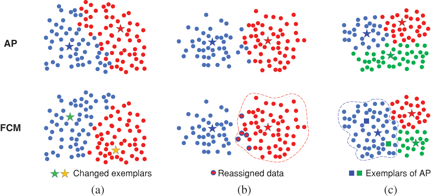
Figure 1: Possible changes in the findings of various clustering approaches. (a) Changes in exemplars. (b) Changes in data assignment. (c) Two exemplars classified in one cluster

By adding a novel constraint and altering the message iteration model, we addressed the foregoing challenge. Then, the adjusted clustering converges stably again based on the new model. Until there are no more conflicting situations, mutual exclusion exemplar detection and clustering of the entire clustering process must be repeated. Some standard classification data sets were adopted to examine and validate the proposed AAEAP algorithm, and six clustering assessment indexes were employed to compare the quality of the result between AAEAP and the other eight clustering algorithms.

The key contributions of the proposed work are as follows:

•   We propose a method that can improve the aggregation ability of AP clustering. The core is to employ a partitioning clustering algorithm to detect mutually exclusive exemplars and then reliably guide AP to combine clusters.

•   The detection information output by the partitioning clustering approach is mapped as a mutual exclusion and aggregation clustering constraint, and the new message iteration model is derived in detail.

•   The overall aggregation improved clustering process is automated and does not need manual intervention, nor does it involve potential exemplar selection and preference revision, which enhances the algorithm’s applicability.

The remainder of this study is organized as follows. Section 2 provides a brief review of AP. Section 3 introduces the proposed AAEAP algorithm. Section 4 presents the experimental findings on standard classification data sets. Section 5 concludes the study work.

2  Affinity Propagation

AP clustering is an exemplar-based clustering algorithm that simultaneously considers all data points as potential exemplars and exchanges messages between them until a high-quality exemplar set and corresponding cluster emerge. AP was originally derived as an instance of the max-product algorithm in a loopy factor graph [19]. A simplified max-sum (log-domain max-product) message update form was obtained by reducing the n-ary messages to binary messages [18,22,23], making the message iteration process of the AP clustering clearer and easier to expand.

Given a data set X={x1,x2,⋯,xN}, a set of exemplars and their clusters are generated through AP clustering. The results are expressed using a binary matrix C={cij}N×Ni,j∈{1,⋯,N}, where cij represents a binary variable, cij = 1, if data point i selects data point j as an exemplar, otherwise cij = 0. If data point i represents an exemplar, then cii = 1, otherwise cii = 0.

The complete process of AP clustering is as follows: First, a data similarity measurement function is defined to compute the similarity s(i,j) between data points xi and xj, which can be a negative Euclidean distance s(i,j)=−‖xi−xj‖2 or user-defined, forming a similarity matrix S={s(i,j)}N×Ni,j∈{1,⋯,N}. The diagonal elements of the similarity matrix S represent preference parameters, denoted as pk=s(k,k),k∈{1,⋯,N}. Based on the S function, Sij is defined to denote the similarity between data points and their exemplars.

Sij(cij)={s(i,j)ifcij=10otherwise(1)

Meanwhile, we provide two basic constraints, I and E. We term I as the 1-of-N constraint, which indicates that each data point can only be assigned to one exemplar. I can be naturally defined as follows:

Ii(ci1,⋯,ciN)={−∞if∑j=1Ncij≠10otherwise(2)

E represents the exemplar consistency constraint, which indicates that once a data point is selected as an exemplar by another point, it must select itself as an exemplar. E is defined as

Ej(c1j,⋯,cNj)={−∞ifcjj=0and∃i≠js.t.cij=10otherwise(3)

Based on Eqs. (1)–(3), the max-sum objective function is expressed as

Fms=∑i=1N∑j=1NSij(cij)+∑i=1NIi(ci1,⋯,ciN)+∑j=1NEj(c1j,⋯,cNj)(4)

As previously mentioned, the max-sum is the representation of the log-domain max-product, and the 1-N constraint and the exemplar consistency constraint in the max-product model are changed as

Ii(ci1,⋯,ciN)={0if∑j=1Ncij≠11otherwise(5)

Ej(c1j,⋯,cNj)={0ifcjj=0and∃i≠js.t.cij=11otherwise(6)

The max-product objective function is expressed as

Fmp=∏i=1N∏j=1NeSij(cij)⋅∏i=1NIi(ci1,⋯,ciN)⋅∏j=1NEj(c1j,⋯,cNj)(7)

The goal of AP clustering is to maximize F by finding a set of exemplars and corresponding data partitions. The process of finding high-quality exemplars is accomplished through the recursive transmission of messages. Fig. 2 shows the transmission mechanisms for the two types of messages, r(i,j) and a(i,j). r(i,j) is referred to as responsibility, which is a message sent by data point i to candidate exemplar j, reflecting the accumulated evidence for how well-suited data point j is to serve as the exemplar for i. a(i,j) is referred to as availability, which represents a message sent by candidate exemplar j to data point i, reflecting the accumulated evidence for how suitable it would be for data point i to select j as its exemplar. In other words, r(i,j) shows how strongly a data point favors one candidate exemplar over other candidates, and a(i,j) shows to what degree each candidate exemplar is available as a cluster center for one data point.

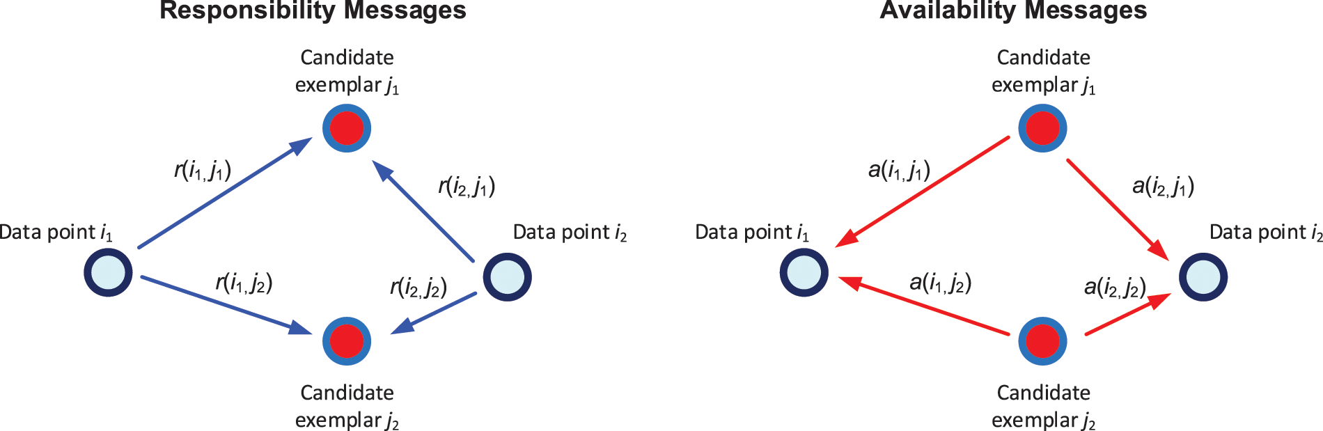
Figure 2: Sending responsibility and availability messages

The messages are initialized as 0 and updated as follows.

∀i,j′r(i,j)=s(i,j)−maxj′≠j⁡[s(i,j′)+a(i,j′)]∀i,j′a(i,j)={∑i′≠imax[0,r(i′,j)],i=jmin[0,r(j,j)+∑i′≠i,jmax[0,r(i′,j)]],i≠j(8)

It is necessary to increase the damping factor λ, with a value range of [0, 1], to prevent oscillation during the message update process. By integrating the message rt and at of the t iteration with the message rt′,at′ based on rt and at, the message rt+1 and at+1 of the t + 1 iteration is obtained.

rt+1(i,j)=(1−λ)⋅rt′(i,j)+λ⋅rt(i,j)at+1(i,j)=(1−λ)⋅at′(i,j)+λ⋅at(i,j)(9)

Responsibility and availability update until convergence. AP ultimately outputs an assignment vector c=[c1,⋯,cN] and ci=argmaxj[r(i,j)+a(i,j)].

3  Automatic Aggregation Enhanced Affinity Propagation

We propose an AAEAP clustering algorithm to overcome the difficulty of AP convergence to a small exemplar size. First, the entire framework of the algorithm is introduced. Then, the basic model is offered, including constraints, objective function, and factor graph. The message iteration is finally derived.

3.1 Overall Framework

The distinctive feature of AAEAP is that it uses a dependable partitioning clustering approach to detect whether there is a mutual exclusion situation in the exemplars produced by AP clustering. If there is, by adding a new constraint, the two mutually exclusive exemplars will not become exemplars and the number of clusters decreases. This will lead to the merging of clusters and present an aggregative state. The algorithm converges to a smaller exemplar size when there are no longer mutually exclusive exemplars. The basic framework of AAEAP is as follows.

The input of the algorithm is an unclassified data set X={x1,⋯,xN}, and each data xi is a one-dimensional sequence having d features. Based on the negative Euclidean distance given by the classic AP, the similarity between two sequences is calculated, and ultimately the similarity matrix S is obtained. The computation approach of the similarity matrix S can be enhanced based on [53,59,60] to make AP more adaptable for data sets with nonspherical structures, although this is not the concentration of this research. The required parameters for AP clustering are initialized, including the maximum iteration number NImax, stable convergence number NIcvg, damping factor λ, and similarity matrix S. It is also required to clarify constraints I and E, which determine the way messages are iterated.

Then, the algorithm enters the message iteration. The algorithm will complete the first convergence based on constraints I and E, and generate a set of XEs containing M exemplars due to the null initialization of the mutually exclusive exemplars MEs. A dependable partitioning clustering approach including K-means, K-medoids, or FCM is used to detect mutually exclusive exemplars in XEs. Particularly, by employing the partitioning clustering approach to generate M clusters simultaneously, each cluster is checked to determine whether there are two or more AP exemplars. If so, the included exemplars are considered mutually exclusive. There may be situations where numerous pairs of mutually exclusive exemplars are detected. Only one pair is randomly selected for each iteration to simplify the computation. The foregoing process of partitioning clustering and detecting is processed through the function IdentifyExclusion, which assigns a pair of mutually exclusive exemplars to MEs.

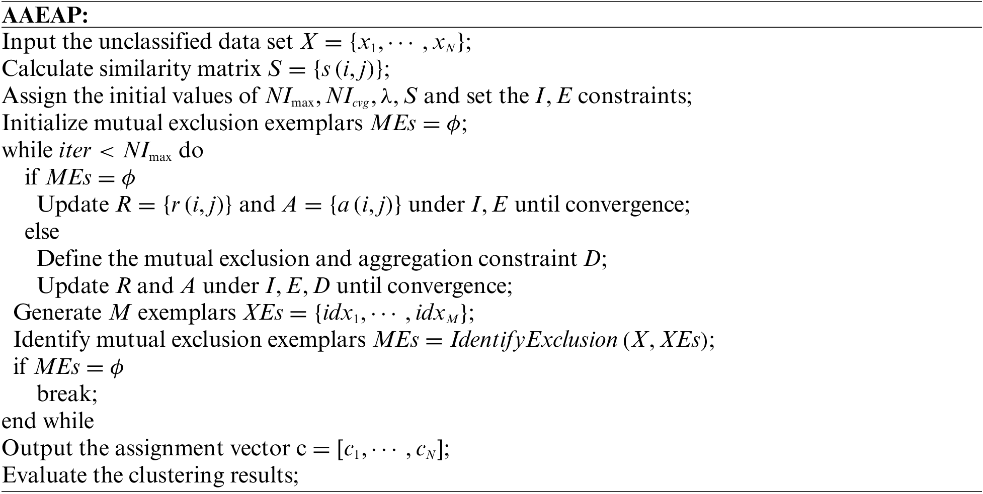
We must define a new constraint D based on MEs, which we call the mutual exclusion and aggregation constraint because of the existence of mutually exclusive exemplars. Its primary capability is to prevent mutually exclusive exemplars from becoming exemplars simultaneously again and reduce the overall number of exemplars by 1. A detailed description will be offered in the next section. The algorithm begins the second message iteration under the constraints of I, E, and D. The expected aggregation impact will occur when stable convergence is achieved. Afterward, the previous steps will be repeated, including detecting the existence of mutually exclusive exemplars, updating constraint conditions D, and restarting message iteration. The algorithm ends until there are no mutually exclusive exemplars left. The output of the AAEAP is the assignment vector c=[c1,⋯,cN], which is the same as the classic AP, and ci=argmaxj[r(i,j)+a(i,j)]. Finally, the clustering results should be examined to confirm the effectiveness of the algorithm.

3.2 Basic Model

Fig. 3 shows the factor graph of the AAEAP algorithm. The similarity function S and the three constraints I, E, and D together influence the variable nodes. The similarity function S only influences each variable node in the graph separately, constraint I influences the rows in the graph, constraint E influences the columns, and constraint D affects the diagonal.

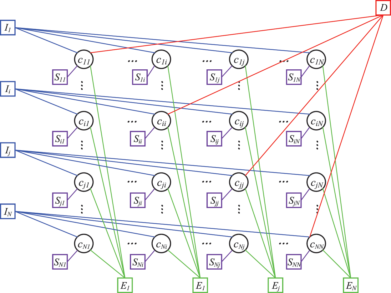
Figure 3: Factor graph of the AAEAP

We present the model of the AAEAP algorithm in the max-product form. First, the constraints of AAEAP are given in detail. The 1-N constraint I and the exemplar consistency constraint E are the same as those of the classic AP. They are defined as

Ii(ci1,⋯,ciN)={0if  ∑j=1Ncij≠11otherwiseEj(c1j,⋯,cNj)={0if  cjj=0  and  ∃i≠ js.t.cij=1 1otherwise(10)

The following concentrates on describing the newly added mutual exclusion and aggregation constraint D. Constraint D has two functions, one of which is to prevent mutually exclusive exemplars from becoming exemplars the next time, that is, they cannot coexist. The next clustering exemplar set XEs will either only have the exemplar p, only exemplar q, or neither exemplars p nor q, assuming that p and q are mutually exclusive exemplars detected and recommended by partitioning clustering. The second function is to cause clustering to aggregation. Exemplars p and q serve as the core and representative of their clusters, reflecting the basic characteristics of the clusters. Crucially, it shows that there are substantial differences in the clusters generated around p and q. Therefore, mutual exclusion can be seen as a problem to the AP clustering findings, showing that some data points of the clusters represented by p and q can be combined, while the remaining data points may select other exemplars, leading to a decrease in 1 in the exemplar number.

According to the above considerations, constraint D is defined as

D(c11,⋯,cNN)={0if∑i=1Ncii≠M−1orcpp⋅cqq=1p,q∈{1,⋯,N}1otherwise(11)

M denotes the exemplar number generated by the previous iteration, p and q are two exemplars that satisfy cpp = 1 and cqq = 1 in the above equation. However, cpp and cqq cannot both be 1, and the exemplar number for the next iteration is constrained to M-1 when they are identified as mutually exclusive exemplars. Constraint D is dynamically changing, as there are three variables p, q, and M, which need to be defined before each iteration to determine the current messaging model.

Then, the max-product objective function defined according to constraints I, E, and D is

Fmp=∏i=1N∏j=1NeSij(cij)⋅∏i=1NIi(ci1,⋯,ciN)⋅∏j=1NEj(c1j,⋯,cNj)⋅D(c11,⋯,cNN)(12)

3.3 Message Iteration

Fig. 4 illustrates the message iteration of AAEAP. As shown in Fig. 4a, there are eight types of messages related to diagonal nodes. As illustrated in Fig. 4b, there are six types of messages related to other nodes.

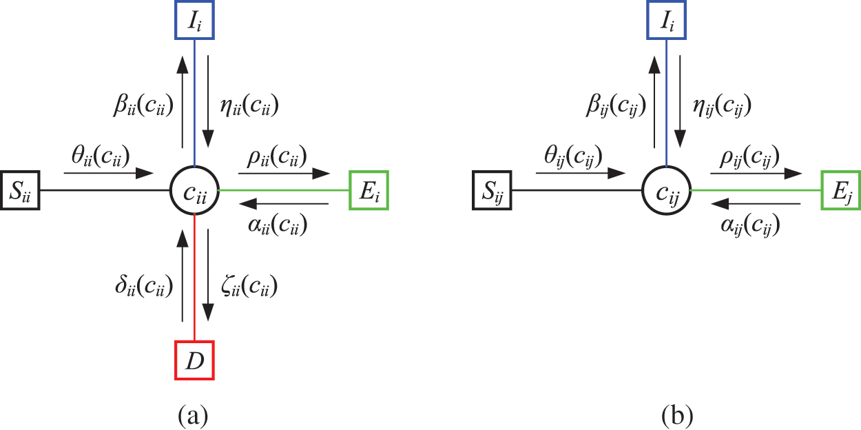
Figure 4: Messages of the AAEAP. (a) Messages associated with cii. (b) Messages associated with cij

Based on the max-product algorithm in the factor graph described in [23,52], the message representation from variable node xi to function node fm is

μxi→fm(xi)=∏fn∈Ne(xi)\fmμfn→xi(xi)(13)

where Ne(xi)\fm represents the set of functions related to the variable xi excluding the function fm, which can be considered as the neighborhood of fm.

The message from function node fm to variable node xi is expressed as

μfm→xi(xi)=max[fm(XNe(fm))⋅∏xj∈Ne(fm)\xiμxj→fm(xj)](14)

where Ne(fm) represents the set of all variable nodes related to the fm function, while Ne(fm)\xi does not include variable xi.

Based on Eq. (13), the messages sent by the variable nodes to the constraint functions in Fig. 4 are

{βii(cii)=μcii→Ii(cii)=δii(cii)⋅θii(cii)⋅αii(cii)βij(cij)=μcij→Ii(cij)=θij(cij)⋅αij(cij)ρii(cii)=μcii→Ei(cii)=δii(cii)⋅θii(cii)⋅ηii(cii)ρij(cij)=μcij→Ej(cij)=θij(cij)⋅ηij(cij)ζii(cii)=μcii→D(cii)=θii(cii)⋅αii(cii)⋅ηii(cii)(15)

Based on Eq. (14), the messages θ sent by the similarity function S to the variable nodes are

{θii(cii)=μSii→cii(cii)=Sii(cii)θij(cij)=μSij→cij(cij)=Sij(cij)(16)

The messages η sent to the variable nodes by the I constraint function are

{ηii(cii)=μIi→cii(cii)=max[Ii(ci1,⋯,cii,⋯,ciN)⋅∏k≠iβik(cik)]ηij(cij)=μIi→cij(cij)=max[Ii(ci1,⋯,cij,⋯,ciN)⋅∏k≠jβik(cik)](17)

The messages α sent by the E constraint function to the variable node are

{αii(cii)=μEi→cii(cii)=max[Ei(c1i,⋯,cii,⋯,cNi)⋅∏k≠iρki(cki)]αij(cij)=μEj→cij(cij)=max[Ej(c1j,⋯,cij,⋯,cNj)⋅∏k≠iρkj(ckj)](18)

Additionally, the δ messages sent by the D constraint function to the variable node are expressed as

δii(cii)=μD→cii(cii)=max[D(c11,⋯,cii,⋯,cNN)⋅∏k≠iζkk(ckk)](19)

The above messages are binary messages that can be normalized by a scalar ratio [23,52]: βij(1)=βij and βij(0)=1. Then

{ηii=ηii(1)ηii(0)=∏k≠iβik(0)maxj≠i[βij(1)⋅∏k≠i,jβik(0)]=βij(0)⋅∏k≠i,jβik(0)maxj≠i[βij(1)⋅∏k≠i,jβik(0)]=1maxj≠iβijηij=ηij(1)ηij(0)=∏k≠jβik(0)maxl≠j[βil(1)⋅∏k≠j,lβik(0)]=1maxl≠jβil=1max{βii,maxl≠i,jβil}(20)

Similarly, ρij(0)=1ρij(1)=ρij and ρij(0)=1, then

{αii=αii(1)αii(0)=max[∏k≠iρki(cki)]∏k≠iρki(0)=∏k≠imax{1,ρki}αij=αij(1)αij(0)=ρjj(1)⋅max[∏k≠i,jρkj(ckj)]max{ρjj(0)⋅∏k≠i,jρkj(0),ρjj(1)⋅max[∏k≠i,jρkj(ckj)]}=min{1,ρjj⋅∏k≠i,jmax{1,ρkj}}(21)

Deriving δii messages is relatively complex, although ζij(1)=ζij and ζij(0)=1, it is crucial to consider both the sub-constraints of mutual exclusion and the reduction of the exemplar number. Suppose p and q are two mutually exclusive exemplars, without loss of generality, if i = p and the exemplar number is reduced to M-1, then

{δii(1)=ζqq(0)⋅max[∏j∈J1ζjj(1)⋅∏k∈K1ζkk(0)]δii(0)=max{ζqq(1)⋅max[∏j∈J1ζjj(1)⋅∏k∈K1ζkk(0)],ζqq(0)⋅max[∏j∈J2ζjj(1)⋅∏k∈K2ζkk(0)]}(22)

Define R={1,⋯,p−1,p+1,⋯,q−1,q+1,⋯,N}. In Eq. (21), J1⊂R has M-2 elements, K1⊂R has N-M elements, and they satisfyJ1∩K1=∅,J1∪K1=R, while J2⊂R has M-1 elements, K2⊂R has N-M-1 elements, and they satisfy J2∩K2=∅,J2∪K2=R. max[∏j∈J1ζjj(1)⋅∏k∈K1ζkk(0)] is the selection of M-2 nodes with a value of 1 and the remaining N-M nodes with a value of 0 from N-2 variable nodes excluding cpp and cqq in the factor graph. This selection scheme can maximize the continuous product of ζjj(1) messages and ζkk(0) messages. Furthermore, it can be obtained that

δii=δii(1)δii(0)=min{1ζqq,max[∏j∈J1ζjj(1)⋅∏k∈K1ζkk(0)]max[∏j∈J2ζjj(1)⋅∏k∈K2ζkk(0)]}=min{1ζqq,max[∏j∈J1ζjj(1)⋅∏k∈K1ζkk(0)]/∏r∈Rζrr(0)max[∏j∈J2ζjj(1)⋅∏k∈K2ζkk(0)]/∏r∈Rζrr(0)}=min{1ζqq,∏r=1M−2ϕr∏r=1M−1ϕr}=min{1ζqq,1ϕM−1}(23)

where Φ represents the ζ message set of ζjj,j∈R messages arranged in descending order, Φ1 represents the maximum value in Φ, and ΦM-1 is the M-1 th largest value in Φ.

And if i∉{p,q}, then

{δii(1)=max[∏j∈J3ζjj(1)⋅∏k∈K3ζkk(0)]δii(0)=max[∏j∈J4ζjj(1)⋅∏k∈K4ζkk(0)](24)

Define R′={1,⋯,i−1,i+1,⋯,N}. In Eq. (23), J3⊂R′,{p,q}⊄J3 has M-2 elements, K3⊂R′ has N-M elements and they satisfy J3 ∩ K3=∅,J3∪K3=R′. Meanwhile, J4⊂R′,{p,q}⊄J4 has M-1 elements, K4⊂R′ has N-M-1 elements and they satisfy J4∩K4=∅,J4∪K4=R′. So

δii=δii(1)δii(0)=max[∏j∈J3ζjj(1)⋅∏k∈K3ζkk(0)]/∏r∈R′ζrr(0)max[∏j∈J4ζjj(1)⋅∏k∈K4ζkk(0)]/∏r∈R′ζrr(0)=∏r=1M−2γr∏r=1M−1γr=1γM−1(25)

where Γ denotes the set of ζ messages arranged in descending order of ζjj,j∈R′ messages. Since p and q are two mutually exclusive exemplars and the min{ζpp,ζqq} element must be eliminated from Γ, ΓM-1 is the M-1 th largest value in Γ.

Through normalization, we have obtained ηii,ηij,αii,αij,δii. Because θij=es(i,j) it is easy to obtain βii=δii⋅θii⋅αii,βij=θij⋅αij, the expressions for other messages are

ζii=θii⋅αii⋅ηii=es(i,i)⋅αii⋅1maxj≠i[es(i,j)⋅αij](26)

{ρii=δii⋅θii⋅ηii=δii⋅es(i,i)⋅1maxj≠iβij=δii⋅es(i,i)⋅1maxj≠i[es(i,j)⋅αij]ρij=θij⋅ηij=es(i,j)⋅1maxl≠jβil=es(i,j)⋅1max{δii⋅es(i,i)⋅αii,maxl≠i,j[es(i,l)⋅αil]}(27)

Responsibility messages are expressed as r(i,j)=log⁡ρij and availability messages are expressed as a(i,j)=log⁡αij [19–23,52]. As a reference, mutual exclusion and aggregation messages are expressed as u(i)=log⁡δii,v(i)=log⁡ζii. They are initialized as 0 and updated, respectively, as follows.

{r(i,i)=u(i)+s(i,i)−maxj≠i[s(i,j)+α(i,j)]r(i,j)=s(i,j)−max{u(i)+s(i,i)+α(i,i),maxl≠i,j[s(i,l)+α(i,l)]}a(i,i)=∑k≠imax{0,r(k,i)}a(i,j)=min{0,r(j,j)+∑k≠i,jmax{0,r(k,j)}}v(i)=s(i,i)+a(i,i)−maxj≠i[s(i,j)+a(i,j)]u(i)={−max{v(q),V′(M−1)},i∈{p,q},i=p−V″(M−1),i∉{p,q}(28)

where V′ represents the set of v(j),j∈R arranged in descending order, and V′(M−1) is the M-1 th largest value in V′. Similarly, V″ represents the set of v(j),j∈R′ arranged in descending order, and V″(M−1) represents the M-1 th largest value in V″.

4  Results and Discussion

The experiments were conducted on some standard classification data sets, and the clustering findings were evaluated using internal and external clustering efficiency evaluation indexes to verify the aggregation and accuracy of AAEAP. The clustering algorithms for comparison include classic AP, five enhanced AP algorithms, SC, and DP.

4.1 Experimental Setting

The data sets for our experiments are from the UC Irvine Machine Learning Repository [61], Knowledge Extraction based on Evolutionary Learning (KEEL) [62], and S-sets [63]. Table 1 presents the brief information on these data sets.

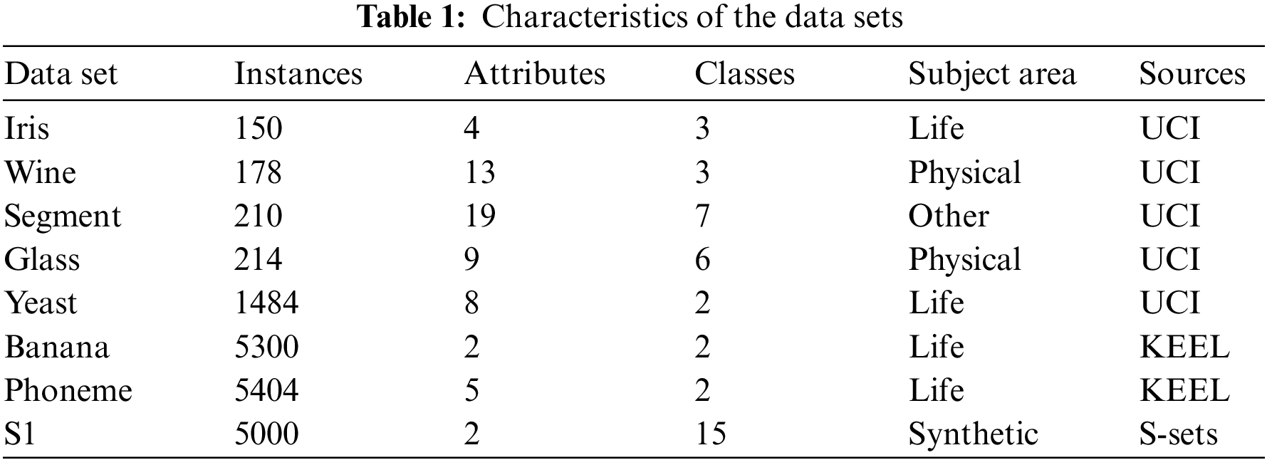
We conduct min-max normalization on each column to ensure that the impact of each attribute on the clustering process and results are balanced before clustering.

xij′=xij−minkxkjmaxkxkj−minkxkj(29)

Besides classic AP, SC, and DP, there are also five enhanced AP algorithms for comparison, including K-AP, AP clustering based on cosine similarity (CSAP) [48], adjusted preference AP clustering based on twice the median (TMPAP) [46], adjusted preference AP clustering based on quantile (QPAP) [50], and adaptive density distribution inspired affinity propagation clustering (ADDAP) [59]. K-AP concentrates on customizing the number of clusters, CSAP concentrates on modifying the similarity matrix S, TMPAP and QPAP concentrate on modifying the preferences, while ADDAP measures the similarities based on nearest neighbor searching and modifies the preferences based on density.

Both the clustering algorithms for comparison and the proposed AAEAP algorithm have been edited and implemented in Matlab R2016b. The pertinent settings are as follows: the similarity between data points is measured by Euclidean distance except for CSAP and ADDAP, the preferences of AAEAP, AP, and CSAP are established as the median of the total inter-point similarities, the damping factors of AAEAP, AP, and five enhanced AP algorithms are 0.9, the M parameter of QPAP is considered the value corresponding to the 5th quantile to reduce the number of exemplars, and the partitioning clustering approach necessary for AAEAP to detect mutually exclusive exemplars is FCM clustering. All experiments were conducted on Windows 7, with Intel® Core™ i7-9700, memory size 16 GB.

4.2 Clustering Evaluations

An integral component of the clustering process is the validation of the clustering findings, and numerous indexes have been proposed to quantitatively evaluate the performance of clustering algorithms. Effectiveness evaluation indexes can be widely classified into two categories: internal and external evaluation indexes. The internal evaluation indexes primarily examine and assess the clustering results from aspects, including compactness, separation, and overlap, based on the structural information of the data set. The external evaluation indexes are mainly based on available prior information from the data set, including the cluster labels of all data points. The performance is evaluated by comparing the degree of correspondence between clustering results and external information.

We use six extensive evaluation indexes, including Silhouette Coefficient (Sil) [64], In-Group Proportion (IGP) [65], Rand Index (RI) [66], Adjusted Rand Index (ARI) [66], F-measure (FM) [67], and Normalized Mutual Information (NMI) [54] to analyze the clustering results of the proposed AAEAP algorithm. Internal evaluation indexes are Sil and IGP, whereas external evaluation indexes are RI, ARI, FM, and NMI.

Sil is an evaluation index based on compactness within a cluster and separation between clusters. For the data point i, compute the average distance from it to other data points within the cluster, denoted as a(i). Compute the average distance from it to each other cluster, and use the minimum value denoted as b(i). Then, its silhouette coefficient can be expressed as

s(i)=(b(i)−a(i))/max{a(i),b(i)}(30)

The value range of s(i) is [−1, 1]. When s(i) approaches 1, it shows that the data point has a high degree of correspondence with the assigned cluster and is distant from other clusters. Furthermore, when s(i) approaches −1, it indicates that the data point is assigned to the wrong cluster. Traditionally, the Sil index of the overall clustering results is the average of s(i) for all data points.

IGP is defined as the proportion of each data point and its nearest neighboring point belonging to the same cluster.

IGP_M=∑u=1ncIGP(u,X)/nc,IGP(u,X)=#{j|ClassX(j)=ClassX(j1NN)=u}#{j|ClassX(j)=u}(31)

where X is the data set, u represents one cluster, j represents a data point in u, j1NN is the nearest neighbor point from j, ClassX(j)=ClassX(j1NN)=u denotes j and j1NN belongs to the same cluster, and # denotes the number of data points that meet the above conditions. Compute IGP(u, X) for all nc clusters, with a larger mean IGP_M showing superior clustering quality.

RI is an external evaluation index that necessitates real classification information C. Assuming K is the clustering results, a denotes the number of data pairs in the same cluster in both C and K, and b denotes the number of data pairs that are not in the same cluster whether in C or K, then RI is expressed as

RI=(a+b)/Cn2(32)

where n represents the number of data points, Cn2 denotes the number of data pairs that can be generated in the data set. The range of RI values is [0,1]. A larger value indicates that the clustering results are more consistent with the real classification.

ARI is an enhancement of RI, which examines clustering by computing the number of data pairs assigned to the same or different clusters in real labels and clustering findings. Compared to RI, ARI has higher discrimination. ARI is expressed as

ARI=2(ad−bc)/[(a+b)(d+b)+(a+c)(d+c)](33)

where a denotes the number of data pairs that belong to the same cluster in both real labels and clustering findings, b denotes the number of data pairs that belong to the same cluster in real labels but do not in clustering findings, c denotes the number of data pairs that do not belong to the same cluster in real labels but belong to the same cluster in clustering findings, and d denotes the number of data pairs that are not in the same cluster, whether in real labels or clustering results. The range of ARI values is [-1, 1], the larger the value, the better the clustering impact, and ARI equals 1, which signifies that clustering findings are completely consistent with real labels.

FM integrates precision and recalls to examine the clustering impact, which is expressed as

F=∑k=1ncnkNmaxm(F(k,m)),F(k,m)=2×precision×recallprecision+recall(34)

where precision=nkm/nk,recall=nkm/nm. nk denotes the number of data points in the k cluster of clustering findings, and nm denotes the number of data points in the m cluster of real classification and nkm denotes the number of data points shared by the k and m clusters. The larger the FM index value, the better the clustering impact.

NMI assesses the similarity between the clustering results and the real labels from the perspective of information theory. Assuming U denotes the clustering results containing k clusters, V denotes the real labels containing m clusters, and MI(U,V) is the mutual information between the clustering results and the real labels, then NMI is expressed as

NMI=MI(U,V)F(H(U),H(V))=∑c=1k∑p=1mncplog⁡(n⋅ncpnc⋅np)/(∑c=1knclog⁡(ncn))(∑p=1mnplog⁡(npn))(35)

where F is the geometric mean, n is the number of data points, nc is the data point number of the c cluster in clustering results, np represents the data point number of the p cluster in real labels, and ncp represents the number of the intersection of the c and p clusters.

4.3 Experimental Results

To demonstrate the automatic aggregation process of the AAEAP algorithm, we selected Iris and Wine data sets. Since the data dimensions of two data sets are greater than 3, we used the classic t-distributed stochastic neighbor embedding (t-SNE) approach [68] to achieve dimensionality reduction and then visualize the data to show the clustering process and aggregation impact.

Fig. 5 demonstrates the findings of the Iris data set. AAEAP converges based on the classic AP when the cluster number NClass is 11. Then, AAEAP iterates eight times to automatically detect mutually exclusive exemplars and aggregates, stably converging to three clusters, consistent with the real category number of the Iris data set.

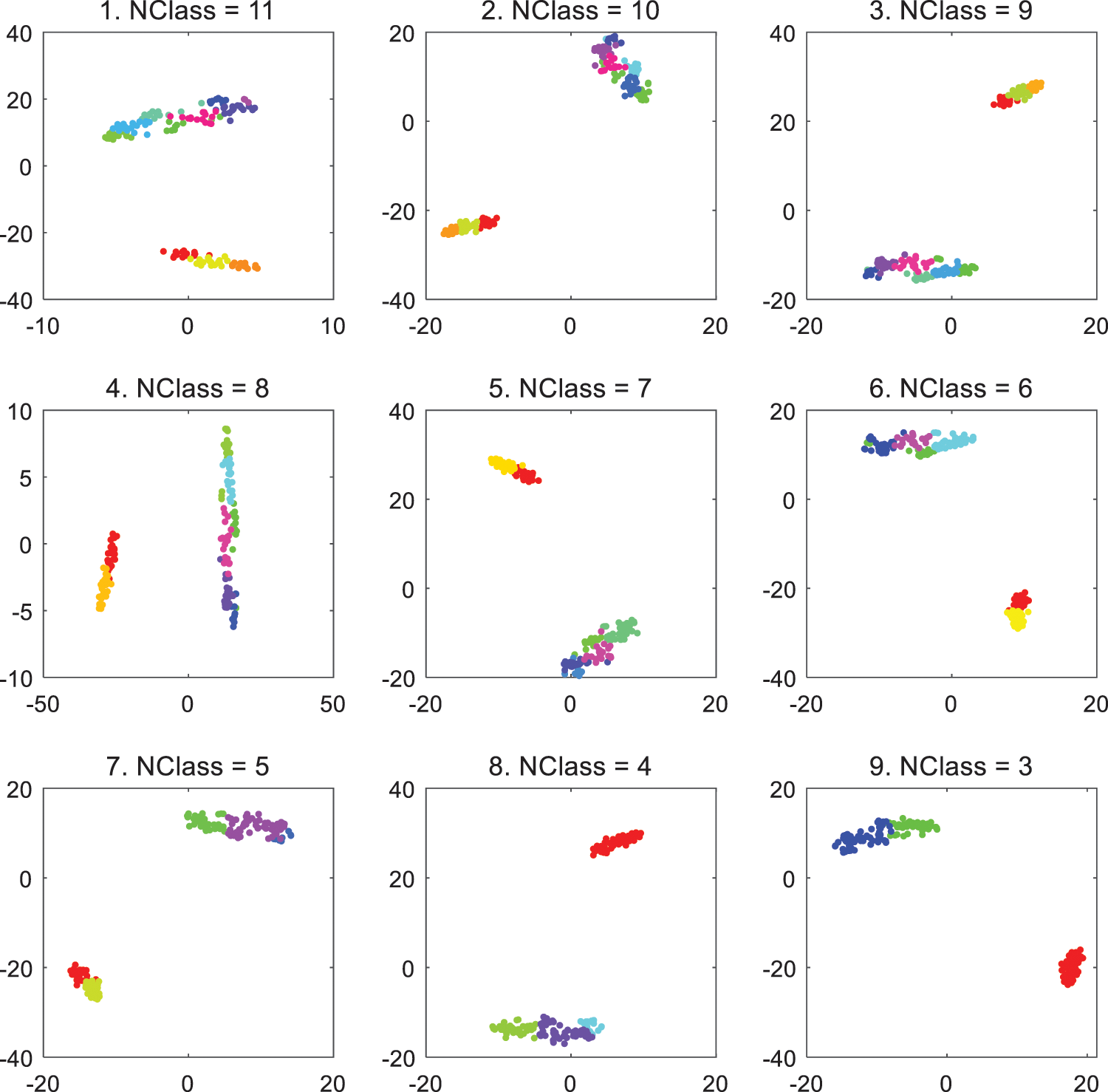
Figure 5: Aggregation effect on Iris data set

Fig. 6 demonstrates the clustering and aggregation impact on the Wine data set. Based on classic AP, AAEAP converges to 21 clusters and then achieves automatic aggregation through mutually exclusive exemplar detection. Finally, with an equivalent number of real categories, AAEAP stably converges into three clusters. However, from the experiments, we discover that AAEAP cannot converge to three clusters every time, and there are also cases of six clusters. Similarly, there are cases of aggregation into three or four clusters for the Yeast data set. The main reason we examined is that AAEAP uses FCM partitioning clustering to detect mutually exclusive exemplars in the experiments, and the random initialization of FCM clustering causes instability in its classification, directly influencing the detection results of mutually exclusive exemplars; therefore, causing changes in AAEAP clustering results. A simple solution is to combine numerous FCM partitioning clustering results to weaken the randomness effect of FCM, and then conduct mutual exclusion detection and ensure the stability and comprehensiveness of the detection. Additionally, it shows the reliability of mutual exclusion detection, which we emphasized earlier. It is easy to imagine that dependable detection will bring accurate aggregation and better clustering quality.

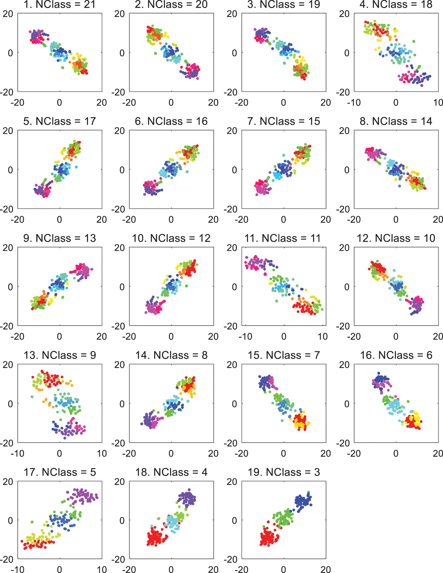
Figure 6: Aggregation effect on Wine data set

Then, to measure the AAEAP clustering quality, we use clustering effectiveness evaluation indexes. Table 2 demonstrates the experimental findings on the Iris, Wine, Yeast, and S1 data sets. AAEAP can converge to the true cluster number, while AP, CSAP, QPAP, and TMPAP cannot. Compared to them, AAEAP has substantial benefits in terms of aggregation performance. ADDAP aims at obtaining the maximum Sil index value, but it cannot obtain the true numbers of clusters for these four data sets. The evaluation indexes of ADDAP are typically superior to those of AP, CSAP, QPAP, and TMPAP. However, AAEAP has better clustering quality than ADDAP, particularly external evaluation indexes, demonstrating that the AAEAP clustering results are closer to the real categories. The evaluation indexes of K-AP, SC, and DP are mostly inferior to those of AAEAP for the Iris, Wine, and Yeast data sets, while their indexes for the S1 data set are perfect and slightly superior to those of AAEAP.

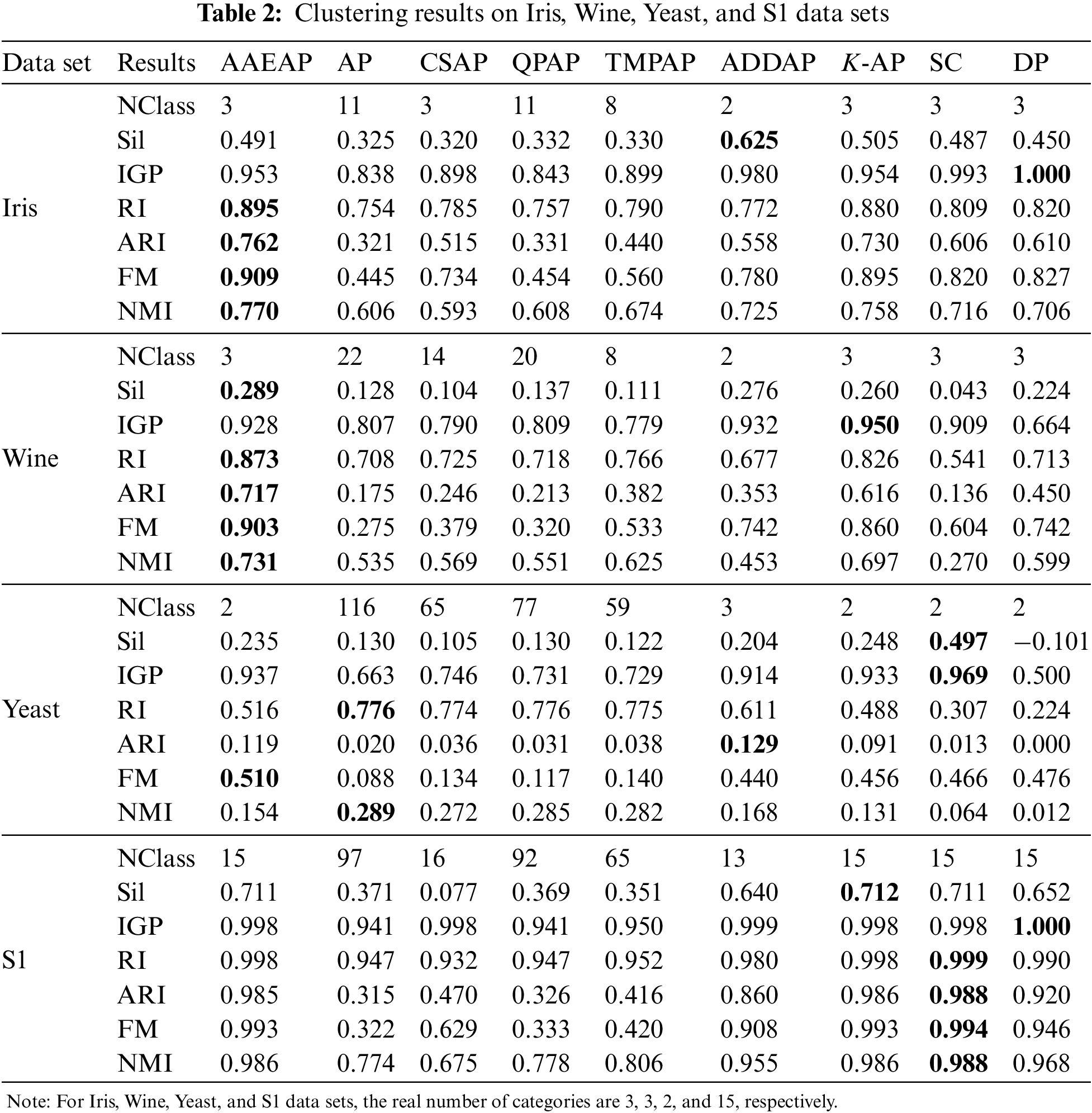
Table 3 shows the findings on Segment and Glass data sets, where AAEAP does not converge to the real category numbers and exhibits excessive aggregation. Therefore, we also delineate the clustering evaluation findings when K-AP, SC, and DP converge to the real category numbers.

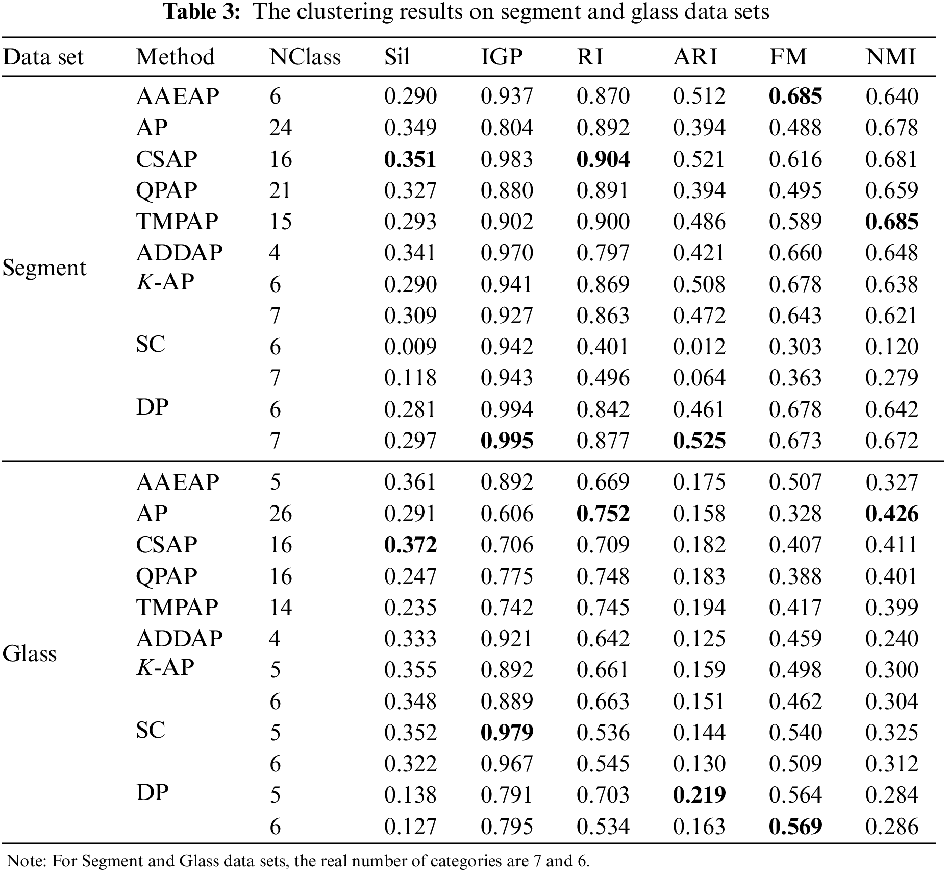
Although the real category number of the Segment data set is 7, Table 3 shows that when K-AP converges into 6 categories, the evaluation indexes are significantly superior to those of 7 categories because of fewer incorrect element classifications, and the entire clustering performance of AAEAP is better than K-AP. However, some evaluation indexes of AP, CSAP, QPAP, and TMPAP are superior to those of AAEAP, but their aggregation performances are poor. The excessive aggregation of ADDAP is more serious, while the evaluation index values are generally good, particularly the internal indexes. The evaluation indexes are mostly inferior to those with seven categories when SC and DP converge into six categories. The performance of AAEAP is superior to that of SC and proximate to DP. The real number of categories is six for the Glass data set, and there is also a situation where the evaluation indexes when K-AP converges into five categories are typically superior to the evaluation indexes with the real category number. Generally, the performance of AAEAP is better than that of K-AP. ADDAP obtains fewer clusters, while its evaluation indexes are often inferior to those of AAEAP. Although AP, CSAP, QPAP, and TMPAP cannot converge into the real number of categories, their evaluation indexes are not bad. The evaluation indexes of SC and DP have their respective benefits, and the index values of AAEAP are often between the two. Fig. 7 demonstrates the entire performance of AAEAP, with no weaknesses in its evaluation indexes. They are substantially superior to the means of indexes obtained by other algorithms and close to the maximum values.

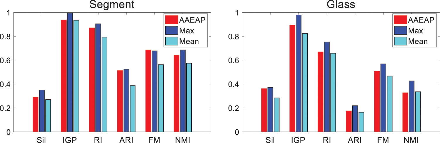
Figure 7: Overall performances of AAEAP on segment and glass data sets

Table 4 shows the findings on Banana and Phoneme data sets, where AAEAP does not converge to the real category numbers and exhibits a lack of aggregation. Therefore, we also delineate the clustering evaluation findings when K-AP, SC, and DP converge to the real category numbers.

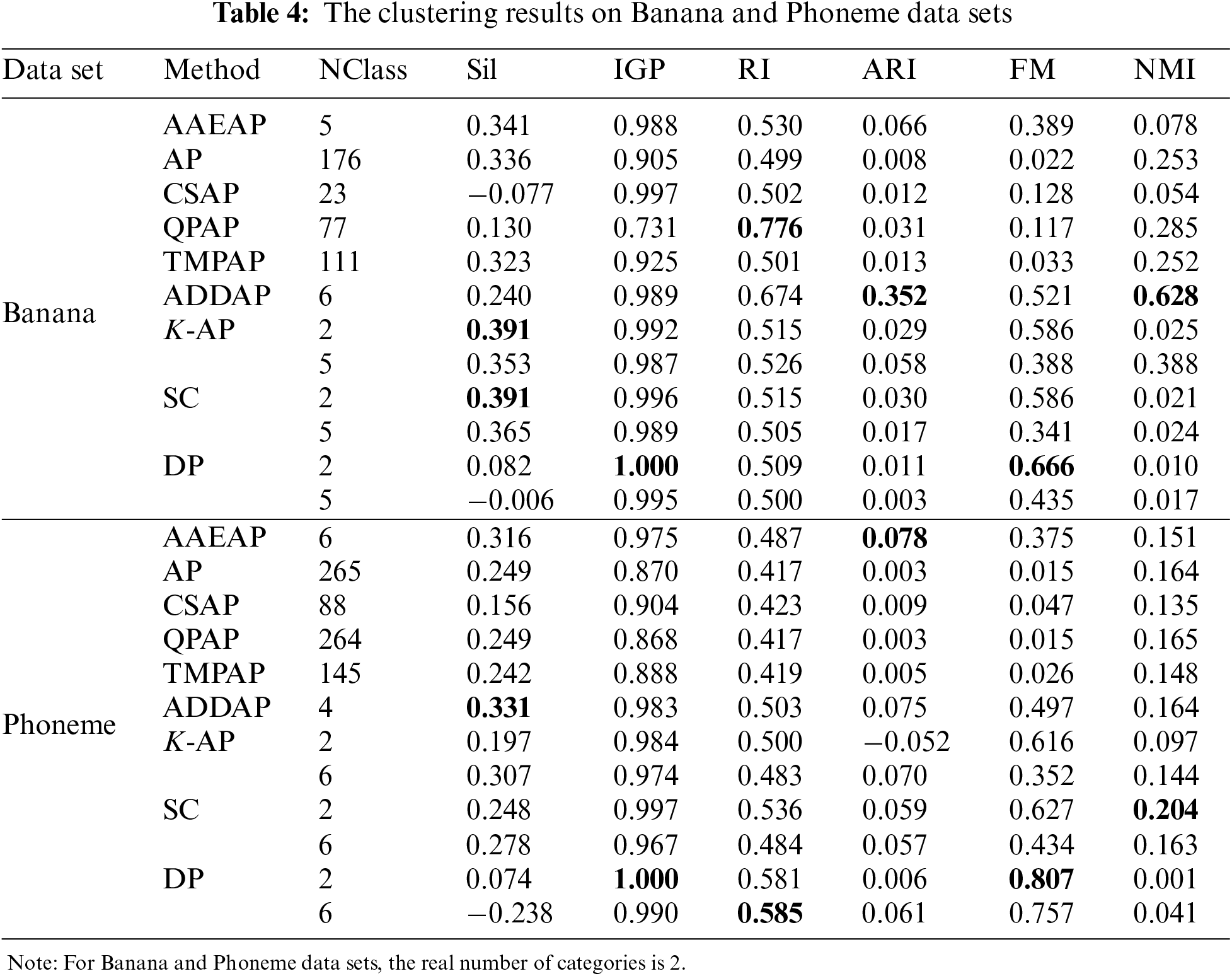
The deviation between the numbers of clusters obtained by AP, CSAP, QPAP, TMPAP, and the real category numbers is significant, and the problem of insufficient aggregation of these four algorithms is obvious. AAEAP converges to the numbers of clusters different from the real numbers since FCM does not offer more mutually exclusive exemplars. However, AAEAP still shows strong automatic aggregation ability even for large data sets compared with AP, CSAP, QPAP, and TMPAP. The performance of ADDAP is superior to that of most algorithms since the density of data is considered and the optimal classification is obtained through iteration. The density distribution is distinctly nonuniform for Banana and Phoneme data sets, enabling ADDAP to offer full play to the superiority. The index values of K-AP, SC, and DP are mostly inferior to those of AAEAP, regardless of whether they obtain the real category numbers or the same number of clusters as AAEAP. Fig. 8 demonstrates the overall performance of AAEAP. The evaluation indexes of AAEAP are superior to the means of indexes obtained by other algorithms and close to the maximum values.

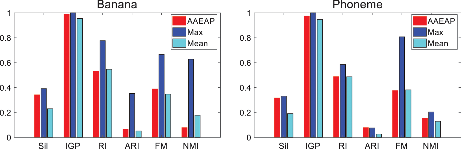
Figure 8: Overall performances of AAEAP on Banana and Phoneme data sets

5  Conclusions

This study proposes an AAEAP clustering algorithm according to mutually exclusive exemplar processing. Its main objective is to enable AP clustering to automatically aggregate, and the information that enhances aggregation comes from real-time partitioning clustering results, rather than prior knowledge or human intervention. This is also the distinction between the AAEAP algorithm and semi-supervised AP clustering algorithms. Potential mutually exclusive exemplar pairs are identified by cross-checking the partitioning and AP clustering findings. Based on them, the current clusters are disassembled and clustering is restarted based on the mutual exclusion and aggregation constraint, achieving aggregation incrementally. From the experimental findings, it can be discerned that the automatic aggregation impact of AAEAP is substantial, and the entire clustering evaluation index values are superior. However, we also discover that the quality of clustering results is related to whether partitioning clustering can offer stable and reliable mutual exclusion detection information. The more accurate the information, the better the AAEAP clustering impact. Future studies will concentrate on enhancing AAEAP to make it more adaptable to cluster on nonspherical data sets.

Acknowledgement: The authors wish to acknowledge the contribution of the Beijing Institute of Tracking and Telemetry Technology, China. The authors also gratefully acknowledge the helpful comments and suggestions of the reviewers.

Funding Statement: This research was supported by Research Team Development Funds of L. Xue and Z. H. Ouyang, Electronic Countermeasure Institute, National University of Defense Technology.

Author Contributions: Study conception and design: Z. H. Ouyang, L. Xue; data collection: Y. S. Duan; analysis and interpretation of results: Z. H. Ouyang, F. Ding; draft manuscript preparation: Z. H. Ouyang, Y. S. Duan. All authors reviewed the results and approved the final version of the manuscript.

Availability of Data and Materials: Data will be made available on request.

Conflicts of Interest: The authors declare that they have no conflicts of interest to report regarding the present study.

References

1. R. Xu and D. C. Wunsch, “Survey of clustering algorithms,” IEEE Transactions on Neural Networks, vol. 16, no. 3, pp. 645–678, 2005. [Google Scholar] [PubMed]

2. Z. Dafir, Y. Lamari and S. C. Slaoui, “A survey on parallel clustering algorithms for big data,” Artifcial Intelligence Review, vol. 54, no. 4, pp. 2411–2443, 2021. [Google Scholar]

3. K. Golalipour, E. Akbari, S. S. Hamidi, M. Lee and R. Enayatifar, “From clustering to clustering ensemble selection: A review,” Engineering Applications of Artificial Intelligence, vol. 104, pp. 104388, 2021. [Google Scholar]

4. A. E. Ezugwu, A. M. Ikotun, O. O. Oyelade, L. Abualigah, J. O. Agushaka et al., “A comprehensive survey of clustering algorithms: State-of-the-art machine learning applications, taxonomy, challenges, and future research prospects,” Engineering Applications of Artificial Intelligence, vol. 110, pp. 104743, 2022. [Google Scholar]

5. A. K. Jain, “Data clustering: 50 years beyond K-means,” Pattern Recognition Letters, vol. 31, no. 8, pp. 651–666, 2010. [Google Scholar]

6. H. S. Park and C. H. Jun, “A simple and fast algorithm for K-medoids clustering,” Expert Systems with Applications, vol. 36, no. 2, pp. 3336–3341, 2009. [Google Scholar]

7. J. C. Bezdek, “Modified objective function algorithms,” in Pattern Recognition with Fuzzy Objective Function Algorithms. Boston, MA, USA: Springer, pp. 155–201, 1981. [Google Scholar]

8. T. Zhang, R. Ramakrishnan and M. Livny, “BIRCH: An efficient data clustering method for very large databases,” ACM SIGMOD Record, vol. 25, no. 2, pp. 103–114, 1996. [Google Scholar]

9. S. Guha, R. Rastogi and K. Shim, “CURE: An efficient clustering algorithm for large databases,” ACM SIGMOD Record, vol. 27, no. 2, pp. 73–84, 1998. https://doi.org/10.1145/276305.276312 [Google Scholar] [CrossRef]

10. M. Ester, H. P. Kriegel, J. Sander and X. W. Xu, “A density-based algorithm for discovering clusters in large spatial databases with noise,” in Proc. of the 2nd Int. Conf. on Knowledge Discovery and Data Mining, Portland, OR, USA, pp. 226–231, 1996. [Google Scholar]

11. M. Ankerst, M. M. Breunig, H. P. Kriegel and J. Sander, “OPTICS: Ordering points to identify the clustering structure,” in Proc. of the 1999 ACM SIGMOD Int. Conf. on Management of Data, Philadelphia, PA, USA, pp. 49–60, 1999. [Google Scholar]

12. A. Rodriguez and A. Laio, “Clustering by fast search and find of density peaks,” Science, vol. 344, no. 6191, pp. 1492–1496, 2014. [Google Scholar] [PubMed]

13. S. H. Yue, M. M. Wei, J. S. Wang and H. X. Wang, “A general grid-clustering approach,” Pattern Recognition Letters, vol. 29, no. 9, pp. 1372–1384, 2008. [Google Scholar]

14. W. Wang, J. Yang and R. Muntz, “STING: A statistical information grid approach to spatial data mining,” in Proc. of the 23rd Int. Conf. on Very Large Data Bases, Athens, Greece, pp. 186–195, 1997. [Google Scholar]

15. R. Agrawal, J. Gehrke, D. Gunopulos and P. Raghavan, “Automatic subspace clustering of high dimensional data,” Data Mining and Knowledge Discovery, vol. 11, no. 1, pp. 5–33, 2005. [Google Scholar]

16. P. D. McNicholas and T. B. Murphy, “Model-based clustering of microarray expression data via latent Gaussian mixture models,” Bioinformatics, vol. 26, no. 21, pp. 2705–2712, 2010. [Google Scholar] [PubMed]

17. U. von Luxburg, “A tutorial on spectral clustering,” Statistics and Computing, vol. 17, no. 4, pp. 395–416, 2007. [Google Scholar]

18. B. J. Frey and D. Dueck, “Clustering by passing messages between data points,” Science, vol. 315, no. 5814, pp. 972–976, 2007. [Google Scholar] [PubMed]

19. F. R. Kschischang, B. J. Frey and H. A. Loeliger, “Factor graphs and the sum-product algorithm,” IEEE Transactions on Information Theory, vol. 47, no. 2, pp. 498–519, 2001. [Google Scholar]

20. Y. Weiss and W. T. Freeman, “On the optimality of solutions of the max-product belief-propagation algorithm in arbitrary graphs,” IEEE Transactions on Information Theory, vol. 47, no. 2, pp. 736–744, 2001. [Google Scholar]

21. C. Yanover, T. Meltzer and Y. Weiss, “Linear programming relaxations and belief propagation—An empirical study,” Journal of Machine Learning Research, vol. 7, pp. 1887–1907, 2006. [Google Scholar]

22. I. E. Givoni and B. J. Frey, “A binary variable model for affinity propagation,” Neural Computation, vol. 21, no. 6, pp. 1589–1600, 2009. [Google Scholar] [PubMed]

23. D. Dueck, “Affinity propagation: Clustering data by passing messages,” Ph.D. dissertation, University of Toronto, Canada, 2009. [Google Scholar]

24. C. H. Du, J. Yang, Q. Wu and T. H. Zhang, “Face recognition using message passing based clustering method,” Journal of Visual Communication and Image Representation, vol. 20, no. 8, pp. 608–613, 2009. [Google Scholar]

25. I. Dagher, S. Mikhael and O. Al-Khalil, “Gabor face clustering using affinity propagation and structural similarity index,” Multimedia Tools and Applications, vol. 80, no. 3, pp. 4719–4727, 2021. [Google Scholar]

26. Y. He, Q. Chen, X. Wang, R. Xu, X. Bai et al., “An adaptive affinity propagation document clustering,” in Proc. of the 7th Int. Conf. on Informatics and Systems, Cairo, Egypt, pp. 1–7, 2010. [Google Scholar]

27. R. C. Guan, X. H. Shi, M. Marchese, C. Yang and Y. C. Liang, “Text clustering with seeds affinity propagation,” IEEE Transactions on Knowledge and Data Engineering, vol. 23, no. 4, pp. 627–637, 2011. [Google Scholar]

28. Z. Q. Zhao, J. Gao, H. Glotin and X. Wu, “A matrix modular neural network based on task decomposition with subspace division by adaptive affinity propagation clustering,” Applied Mathematical Modelling, vol. 34, no. 12, pp. 3884–3895, 2010. [Google Scholar]

29. J. Zhang, X. Tuo, Z. Yuan, W. Liao and H. Chen, “Analysis of fMRI data using an integrated principal component analysis and supervised affinity propagation clustering approach,” IEEE Transactions on Biomedical Engineering, vol. 58, no. 11, pp. 3184–3196, 2011. [Google Scholar] [PubMed]

30. H. M. Ge, L. G. Wang, H. Z. Pan, Y. X. Zhu, X. Y. Zhao et al., “Affinity propagation based on structural similarity index and local outlier factor for hyperspectral image clustering,” Remote Sensing, vol. 14, no. 5, pp. 1995, 2022. [Google Scholar]

31. X. L. Zhang, C. Furtlehner, C. Germain and M. Sebag, “Data stream clustering with affinity propagation,” IEEE Transactions on Knowledge and Data Engineering, vol. 26, no. 7, pp. 1644–1656, 2014. [Google Scholar]

32. Q. H. Gao, Y. W. Wang, X. Z. Cheng, J. G. Yu, X. Chen et al., “Identification of vulnerable lines in smart grid systems based on affinity propagation clustering,” IEEE Internet of Things Journal, vol. 6, no. 3, pp. 5163–5171, 2019. [Google Scholar]

33. J. Zhang, X. Tuo, Z. Yuan, W. Liao and H. Chen, “A practical semi-dynamic clustering scheme using affinity propagation in cooperative picocells,” IEEE Transactions on Vehicular Technology, vol. 64, no. 9, pp. 4372–4377, 2015. [Google Scholar]

34. L. Wang, Y. J. Zhang and S. S. Zhong, “Typical process discovery based on affinity propagation,” Journal of Advanced Mechanical Design, Systems, and Manufacturing, vol. 10, no. 1, pp. 1–13, 2016. [Google Scholar]

35. Z. X. Wei, Y. X. Wang, S. L. He and J. D. Bao, “A novel intelligent method for bearing fault diagnosis based on affinity propagation clustering and adaptive feature selection,” Knowledge-Based Systems, vol. 116, no. C, pp. 1–12, 2017. [Google Scholar]

36. Q. Hu, Q. Zhang, X. S. Si, G. X. Sun and A. S. Qin, “Intelligent fault diagnosis approach based on composite multi-scale dimensionless indicators and affinity propagation clustering,” IEEE Sensors Journal, vol. 20, no. 19, pp. 11439–11453, 2020. [Google Scholar]

37. M. Li, Y. X. Wang, Z. G. Chen and J. Zhao, “Intelligent fault diagnosis for rotating machinery based on potential energy feature and adaptive transfer affinity propagation clustering,” Measurement Science and Technology, vol. 32, no. 9, pp. 94012, 2021. [Google Scholar]

38. J. X. Bi, Y. J. Wang, X. Li, H. X. Qi, H. J. Cao et al., “An adaptive weighted KNN positioning method based on omnidirectional fingerprint database and twice affinity propagation clustering,” Sensors, vol. 18, no. 8, pp. 2502, 2018. [Google Scholar] [PubMed]

39. M. J. Brusco, D. Steinley, J. Stevens and J. D. Cradit, “Affinity propagation: An exemplar-based tool for clustering in psychological research,” British Journal of Mathematical and Statistical Psychology, vol. 72, no. 1, pp. 155–182, 2019. [Google Scholar] [PubMed]

40. H. Y. Xia, S. Zha, J. J. Huang and J. B. Liu, “Radio environment map construction by adaptive ordinary Kriging algorithm based on affinity propagation clustering,” International Journal of Distributed Sensor Networks, vol. 16, no. 5, pp. 1–10, 2020. [Google Scholar]

41. Y. M. Han, C. Y. Fan, Z. Q. Geng, B. Ma, D. Cong et al., “Energy efficient building envelope using novel RBF neural network integrated affinity propagation,” Energy, vol. 209, pp. 118414, 2020. [Google Scholar]

42. S. Sajid, L. Chouinard and N. Carino, “Condition assessment of concrete plates using impulse-response test with affinity propagation and homoscedasticity,” Mechanical Systems and Signal Processing, vol. 178, pp. 109289, 2022. [Google Scholar]

43. L. C. Wang, Y. S. Chao, S. H. Cheng and Z. Han, “An integrated affinity propagation and machine learning approach for interference management in drone base stations,” IEEE Transactions on Cognitive Communications and Networking, vol. 6, no. 1, pp. 83–94, 2020. [Google Scholar]

44. A. Busch, T. H. Bachmann, M. Y. Abdel-Glil, A. Hackbart, H. Hotzel et al., “Using affinity propagation clustering for identifying bacterial clades and subclades with whole-genome sequences of Francisella tularensis,” PLoS Neglected Tropical Diseases, vol. 14, no. 9, pp. e0008018, 2020. [Google Scholar] [PubMed]

45. X. F. Yan, H. Chen, H. R. Huang, Q. Liu and M. Yang, “Building typification in map generalization using affinity propagation clustering,” ISPRS International Journal of Geo-Information, vol. 10, no. 11, pp. 732, 2021. [Google Scholar]

46. S. H. Xu, Z. J. Qin, W. T. Zhang, X. M. Xiong, H. Li et al., “A novel method of recognizing disturbance events in Φ-OTDR based on affinity propagation clustering and perturbation signal selection,” IEEE Sensors Journal, vol. 21, no. 12, pp. 13272–13282, 2021. [Google Scholar]

47. P. M. Harikrishnan, A. Thomas, V. P. Gopi, P. Palanisamy and K. A. Wahid, “Inception single shot multi-box detector with affinity propagation clustering and their application in multi-class vehicle counting,” Applied Intelligence, vol. 51, no. 7, pp. 4714–4729, 2021. [Google Scholar]

48. A. Alitaleshi, H. Jazayeriy and J. Kazemitabar, “Affinity propagation clustering-aided two-label hierarchical extreme learning machine for Wi-Fi fingerprinting-based indoor positioning,” Journal of Ambient Intelligence and Humanized Computing, vol. 13, no. 6, pp. 3303–3317, 2022. [Google Scholar]

49. M. Katebi, A. RezaKhani, S. Joudaki and M. E. Shiri, “RAPSAMS: Robust affinity propagation clustering on static android malware stream,” Concurrency and Computation: Practice and Experience, vol. 34, no. 15e6980, 2022. [Google Scholar]

50. X. Fang, C. S. Luo, D. R. Zhang, H. F. Zhang, J. Qian et al., “Pre-selection of monitoring stations for marine water quality using affinity propagation: A case study of Xincun Lagoon, Hainan, China,” Journal of Environmental Management, vol. 325, pp. 116666, 2023. [Google Scholar] [PubMed]

51. X. Guo, Z. X. Yang, C. Li, H. X. Xiong and C. M. Ma, “Combining the classic vulnerability index and affinity propagation clustering algorithm to assess the intrinsic aquifer vulnerability of coastal aquifers on an integrated scale,” Environmental Research, vol. 217, pp. 114877, 2023. [Google Scholar] [PubMed]

52. X. L. Zhang, W. Wang, K. Nørvåg and M. Sebag, “K-AP: Generating specified K clusters by efficient affinity propagation,” in Proc. of 2010 IEEE Int. Conf. on Data Mining, Sydney, NSW, Australia, pp. 1187–1192, 2010. [Google Scholar]

53. F. H. Shang, L. C. Jiao, J. R. Shi, F. Wang and M. G. Gong, “Fast affinity propagation clustering: A multilevel approach,” Pattern Recognition, vol. 45, no. 1, pp. 474–486, 2012. [Google Scholar]

54. C. D. Wang, J. H. Lai, C. Y. Suen and J. Y. Zhu, “Multi-exemplar affinity propagation,” IEEE Transactions on Pattern Analysis and Machine Intelligence, vol. 35, no. 9, pp. 2223–2237, 2013. [Google Scholar] [PubMed]

55. D. W. Chen, J. Q. Sheng, J. J. Chen and C. D. Wang, “Stability-based preference selection in affinity propagation,” Neural Computing and Applications, vol. 25, no. 7, pp. 1809–1822, 2014. [Google Scholar]

56. N. M. Arzeno and H. Vikalo, “Semi-supervised affinity propagation with soft instance-level constraints,” IEEE Transactions on Pattern Analysis and Machine Intelligence, vol. 37, no. 5, pp. 1041–1052, 2015. [Google Scholar] [PubMed]

57. L. L. Sun, C. H. Guo, C. R. Liu and H. Xiong, “Fast affinity propagation clustering based on incomplete similarity matrix,” Knowledge and Information Systems, vol. 51, no. 3, pp. 941–964, 2017. [Google Scholar]

58. P. Li, H. F. Ji, B. L. Wang, Z. Y. Huang and H. Q. Li, “Adjustable preference affinity propagation clustering,” Pattern Recognition Letters, vol. 85, pp. 72–78, 2017. [Google Scholar]

59. Z. Y. Fan, J. Jiang, S. Q. Weng, Z. H. He and Z. W. Liu, “Adaptive density distribution inspired affinity propagation clustering,” Neural Computing and Applications, vol. 31, no. 1, pp. 435–445, 2019. [Google Scholar]

60. L. Tang, L. L. Sun, C. H. Guo and Z. Zhang, “Adaptive spectral affinity propagation clustering,” Journal of Systems Engineering and Electronics, vol. 33, no. 3, pp. 647–664, 2022. [Google Scholar]

61. UCI Datasets, 2007. [Online]. Available: https://archive-beta.ics.uci.edu/datasets [Google Scholar]

62. J. Alcalá-Fdez, A. Fernandez, J. Luengo, J. Derrac, S. García et al., “KEEL data-mining software tool: Data set repository, integration of algorithms and experimental analysis framework,” Journal of Multiple-Valued Logic and Soft Computing, vol. 17, no. 2–3, pp. 255–287, 2011. [Google Scholar]

63. P. Fränti and O. Virmajoki, “Iterative shrinking method for clustering problems,” Pattern Recognition, vol. 39, no. 5, pp. 761–775, 2006. [Google Scholar]

64. P. J. Rousseeuw, “Silhouettes: A graphical aid to the interpretation and validation of cluster analysis,” Journal of Computational and Applied Mathematics, vol. 20, no. 1, pp. 53–65, 1987. [Google Scholar]

65. A. V. Kapp and R. Tibshirani, “Are clusters found in one dataset present in another dataset?” Biostatistics, vol. 8, no. 1, pp. 9–31, 2007. [Google Scholar] [PubMed]

66. A. D’Ambrosio, S. Amodio, C. Iorio, G. Pandolfo and R. Siciliano, “Adjusted concordance index: An extensionl of the adjusted rand index to fuzzy partitions,” Journal of Classification, vol. 38, no. 1, pp. 112–128, 2021. [Google Scholar]

67. L. M. Wang, Q. Ji and X. M. Han, “Adaptive semi-supervised affinity propagation clustering algorithm based on structural similarity,” Tehnicki Vjesnik, vol. 23, no. 2, pp. 425–435, 2016. [Google Scholar]

68. L. J. P. van der Maaten and G. E. Hinton, “Visualizing data using t-SNE,” Journal of Machine Learning Research, vol. 9, pp. 2579–2605, 2008. [Google Scholar]