VGWO: Variant Grey Wolf Optimizer with High Accuracy and Low Time Complexity

1  Introduction

This section first introduces why we conduct this research through background and motivation in Section 1.1. Then we present our contribution in Section 1.2.

1.1 Background and Motivation

With the development of society, human beings have increasingly higher requirements for the accuracy of engineering design, structural optimization, task scheduling, and other practical engineering applications and scientific research. In the process of conducting the above research, many excellent algorithms have been generated in recent years. For example, the grey wolf optimizer (GWO) [1], the Equilibrium optimizer [2], the Artificial hummingbird algorithm [3], the Multi-trial vector-based monkey king evolution algorithm [4], and so on. They have been shown to outperform many intelligent optimization algorithms and are applied to different engineering optimization problems. However, as the research progressed, many limitations of intelligent optimization algorithms were identified. For example, Zaman et al. used the powerful global exploration capability of the backtracking search optimization algorithm to enhance the convergence accuracy of particle swarm optimization (PSO) [5]. Shen et al. optimized the convergence speed of the whale optimization algorithm by dividing the fitness into three subpopulations [6].

The grey wolf optimizer (GWO) [1] is a swarm-based intelligence optimization algorithm proposed by Mirjalili et al. in 2014. GWO solves the optimization problem by simulating the steps of searching, encircling, and attacking prey in the process of wolf hunting. The first two stages (i.e., searching and encircling) make a global search, and the last stage (i.e., attacking) takes a local search. The social hierarchy of wolves is classified into four types (i.e., α, β, δ, and ω) according to their fitness, where α wolf has the highest social rank, and ω wolf has the lowest social rank. Compared with other optimization algorithms, GWO can adaptively adjust the convergence factor and information feedback to achieve a balance between local optimization and global search, so it has good performance in terms of problem-solving. GWO has been successfully applied to the fields of job shop scheduling [7], parameter optimization [8], and image detection [9] due to its advantages of a simple principle and a few parameters that need adjustment.

Despite the merits mentioned above, concerning the solution accuracy and the searching ability, the original GWO has a potential space to improve. In addition, there is a paradox in GWO: the social rank values of α, β, and δ are different in accordance with the design of the social hierarchy, but these values are the same in practice. In response to the above questions, Some advanced GWOs have been proposed recently, including variable weight GWO (VWGWO) [10], PSO combined with GWO (PSOGWO) [11], and covariance matrix adaptation with GWO (CMAGWO) [12]. VWGWO strengthens the leadership of α. PSOGWO accelerates the convergence of populations at later stages. CMAGWO can enhance a local search for wolves. Although these algorithms make some improvements to GWO, they still have the following limitations:

1)   Low accuracy solution. During the initialization population phase, GWO, VWGWO, and CMAGWO generate wolves randomly; this mechanism cannot guarantee the diversity of the population. Although PSOGWO uses Tent mapping to make the initial population more uniformly distributed, however, due to the fixed mapping period of the Tent mapping, the randomness in the initialization phase still has room to improve. Meanwhile, in our observation, PSOGWO does not remarkably improve the solution quality because of the two fundamental optimizers’ common drawbacks of falling into local optimum.

2)   Unreasonable weight setting. During the searching phase, VWGWO sets the weight of α close to 1, whereas the weights of β and δ are close to 0. This setting will untimely establish the α wolf’s dominance and weaken the leadership of β and δ. Thus, VWGWO easily leads to early convergence to α and falls into a local optimum.

3)   High time complexity. In CMAGWO, if the GWO solution quality is poor, then the CMA-ES optimization space is extremely limited. In addition, CMA-ES needs to decompose the covariance matrix during iteration (its complexity is as high as O(N3), where N denotes the number of wolves), and CMAGWO significantly increases the running time compared with GWO.

1.2 Our Contributions

To solve the aforementioned problems, this paper proposes a high-accuracy variable GWO (VGWO) while still with low time complexity in this study. The contributions are listed below:

1)   A mechanism to improve population diversity is developed. Several pairs of wolves with symmetric relationships are added to the population during the wolves’ initialization stage. The diversity of the wolves increases and further makes the wolves’ distribution more uniform. This scheme is easy to implement and can be applied to problems of different scales.

2)   A method to prevent wolves from premature convergence is designed. Dynamically adjusting the weights of α, β, and δ improves the convergence speed and solution accuracy of wolves.

3)   A notion to make wolves jump out of the local optimum is presented. Random perturbations are leveraged to delay the gathering of the wolves and strengthen the random search ability of the algorithm while keeping the algorithm in a low time complexity.

4)   Some evaluations are conducted to illustrate the VGWO’s advantages. VGWO, GWO, PSOGWO, VWGWO, and CMAGWO are evaluated by 19 benchmark functions and 3 engineering cases. Compared to the state-of-art GWOs and CEC2020 competition winner, the experimental results illustrate that VGWO has good solution quality and fast convergence speed without increasing the time complexity. A further evaluation based on the Friedman test, VGWO also outperforms all other algorithms statistically in terms of robustness with a better average ranking value.

The remainder of this article is as follows: Section 2 reviews the work related to GWO. Section 3 describes the VGWO model and its derivation process. Section 4 gives the parameter settings of different algorithms in the experiments. Section 5 first conducts the experiments on benchmark functions, followed by the analysis of the experimental results, and further demonstrates the excellence of VGWO by comparing its performance with the CEC2020 winner. Section 6 evaluates VGWO through three different engineering examples. Section 7 summarizes the work of this study and provides suggestions for further research.

2  Related Work

Many researchers have made relevant improvements to address the shortcomings of GWO. Work related to GWO focuses on three perspectives, namely, the initialization population of GWO, the search mechanism of GWO, and hybridizing other metaheuristics of GWO.

1)   Population Initialization of GWO. The outcome of the initialization population affects the quality and speed of convergence. However, wolves in the original GWO are generated randomly, so their diversity cannot be guaranteed. Long et al. [13] first introduced the point set theory in GWO, which initializes the population and makes wolves’ distribution more uniform to solve this problem. Luo et al. [14] employed complex numbers to code the grey wolf individuals. This method can increase the amount of information in the gene because a complex number has 2D properties. Kohli et al. [15] developed a GWO based on chaotic sequences and demonstrated that their method has greater stability than GWO. Similarly, Teng et al. [11] suggested a particle swarm optimization combined with GWO (PSOGWO), which increases the randomness of initialized populations by Tent mapping. However, the foregoing research only considers the effects of the starting population and ignores the balance between local and global search capabilities.

2)   Searching Mechanism of GWO. A number of studies about search mechanisms focus on the enhancement of control parameter a (a is used to control the proportion of global and local search) or on the calculation method of individual coordinates. Saremi et al. [16] combined GWO with evolutionary population dynamics (EPD), where EPD can remove the poor solution and reposition it around α, β, or δ to improve GWO’s local search ability. Mittal et al. [17] proposed a modified GWO (mGWO) that adjusts the control parameter a to improve the effectiveness and stability of GWO. Lu et al. [18] increased the topological neighbors of wolves to ensure population diversity by combining GWO with topology. However, the weight of dominant wolves (α, β, and δ) contradicts their social hierarchy and affects the GWO’s performance. Considering this problem, Gao et al. [10] proposed a variable weight GWO to reduce the probability of GWO falling into the local optimum. However, VWGWO’s solution quality does not improve much compared to GWO because it overemphasizes the weight of α.

3)   Hybrid Metaheuristics of GWO. GWO also has gained popularity in the field of hybrid metaheuristics, with many researchers combining it with differential evolution (DE) or PSO. Yao et al. [19] used the survival of the fittest strategy from DE and presented an improved GWO. Similarly, Zhu et al. [20] proposed a hybrid GWO with DE to improve the GWO’s global search ability. Contrary to reference [20], Jitkongchuen [21] proposed a hybrid DE algorithm with GWO (jDE). jDE employs the GWO’s coordinate update strategy to improve the crossover operator in DE. However, since PSO introduces the historical optimal solution into the algorithm, thereby obtaining strong convergence [22], Singh et al. [23] observed that the above GWOs do not account for wolves’ historical optimal coordinates, so they proposed a hybrid GWO based on PSO (HPSOGWO). HPSOGWO has better exploratory ability than GWO; PSOGWO is developed based on HPSOGWO. Zhao et al. [12] used a two stage search to improve the GWO’s local search ability and then designed a covariance matrix adaptation with GWO (CMAGWO).

Meanwhile, GWO plays a very important role in the application of engineering problems. In the field of parameter optimization, Madadi et al. [24] used the GWO algorithm to design a new optimal proportional-integral-derivative (PID) controller, then compared the PID-GWO and PID-PSO controllers; the results showed that the PID-GWO can better improve the dynamic performance of the system. Lal et al. [25] employed GWO algorithm to optimize the fuzzy PID controller and applied it to the automatic control of the interconnected hydrothermal power system. Sweidan et al. [26] leveraged GWO to optimize the parameters of the support vector machine (SVM) and used the optimized SVM to assess water quality; Eswaramoorthy et al. [27] utilized GWO to tune the SVM classifier and used it for a case study of intracranial electroencephalography (iEEG) signal classification middle. Muangkote et al. [28] applied the improved GWO algorithm to the training of q-Gaussian-based radial basis function logic network (RBFLN) neural network and pointed out that the improved GWO algorithm has higher accuracy in solving complex problems through comparative experiments; Mirjalili et al. [29] first used GWO to train multi-layer perceptron (MLP). Compared with other well-known algorithms, GWO-MLP can effectively avoid falling into local optimum. Al-Shaikh et al. [30] used GWO to find strongly connected components in directed graphs in linear time, addressing the serious time-consuming shortcomings of Tarjan's algorithm and the Forward-Backward algorithm. In the field of renewable energy systems, Sivarajan et al. [31] made use of GWO to determine the optimal feasible solution to the dynamic economic dispatch problem of combined heat and power generation considering wind farms and tested the performance of the GWO algorithm with a test system containing 11 generating units. The results show that the GWO algorithm is superior in both economy and computing time. Mohammad et al. [32] used GWO to solve the problem of photovoltaic solar cells and greatly reduced the waste of energy by estimating the performance. In addition, Almazroi et al. applied GWO to an implicit authentication method for smartphone users [33]. Zaini et al. predicted the energy consumption of home appliances through GWO [34].

Although the above GWOs have some advantages in different parts, they mainly focus on optimizing the internal shortcomings of wolf individuals. This study continues to analyze GWO. Different from the above algorithm, our work focuses on trying to leverage multiple mechanisms to improve the quality of the solution.

3  Design of VGWO Algorithm

This section first introduces VGWO in detail. Then, an outline of three aspects is presented, followed by a detailed description of the algorithmic flow. All variants used in this study and their corresponding definitions, as well as the time complexity analysis of VGWO, are also introduced in this section.

3.1 Enhancing Wolves’ Diversity through Symmetrical Wolf (SW)

In GWO, initializing the population is a crucial stage. A healthy population has a direct influence on the speed and outcome of convergence in general. However, the original GWO population initialization was performed at random, which cannot guarantee a good diversity of wolves, thereby decreasing the algorithm’s effectiveness. This paper gives a definition named SW to overcome this drawback and then focuses on how SW be used to start populations.

Definition 1: SW. Wolf individual’s symmetric coordinates about the center of the search range.

We briefly describe the above definition through an example. Assuming that a point x∈[l,r] exists in the 1D space, and the SW point of x is the symmetrical point of x about the symmetry center o=l+r2. When extending to 3D space, for example, a point x = (1, 2, 3) is found in Fig. 1, where the search range is {(x,y,z)|x∈[−5,5],y∈[−5,5],z∈[−5,5]}, that is, the green space in Fig. 1. Thus, the symmetry center is (0, 0, 0), and the SW point of x in the search range is x’ = (−1, −2, −3).

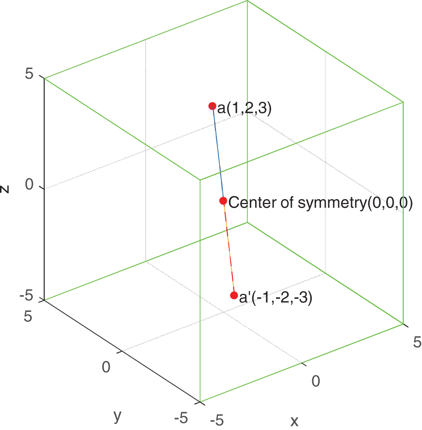
Figure 1: SW point in three-dimensional space (1,2,3)

Combined with Definition 1, the steps of initializing an individual coordinates solution using SW are as follows: 1) Initialize the coordinates X→i (i = 1, 2, ···, N) of N grey wolf individuals in the defined domain space as the initialization wolves ini_population; 2) Generate the SW population sym_population of population ini_population in accordance with Definition 1; 3) Merge populations ini_population and sym_population to obtain population, and then sort population by fitness value; 4) Select the first N individuals as the initial population.

The pseudo-code of the initialized population is shown in Algorithm 1, where N and dim indicate the amount and dimension of the population, respectively, and [l, r] represents the search range of wolves. The initialized individuals obey the beta distribution because the beta distribution can generate as many non-edge individuals as possible, thereby improving the search efficiency of GWO. With the use of SW constraint in Algorithm 1, the diversity of the wolves is enhanced considerably. The search for SW and the initialization of the population are performed simultaneously, which has minimal effect on the time complexity of the algorithm.

The SW implementation is simple and scalable. Thus, it can be applied after each wolf’s coordinate update. Figs. 2 and 3 show the wolves after seeking for SWs in the searching and encircling phases, respectively. The black dot in the figure is assumed to be the search range’s center, α’, β’, and δ’ are correspondingly the SWs of α, β, and δ. The grey point represents an ordinary wolf who will move toward α, β, and δ, and the yellow point represents the prey. As shown in Fig. 2, SW increases wolf diversity and has the potential to bring wolves closer to their prey. However, the wolves begin to round up the prey, as shown in Fig. 3. If we search SW for the entire population as usual, then the generated SW wolves will be far away from the prey, which is obviously an invalid operation. Thus, the wolves must generate SW wolves adaptively at various stages. In short, VGWO will reduce the SW wolf search when the wolves reach the encirclement phase.

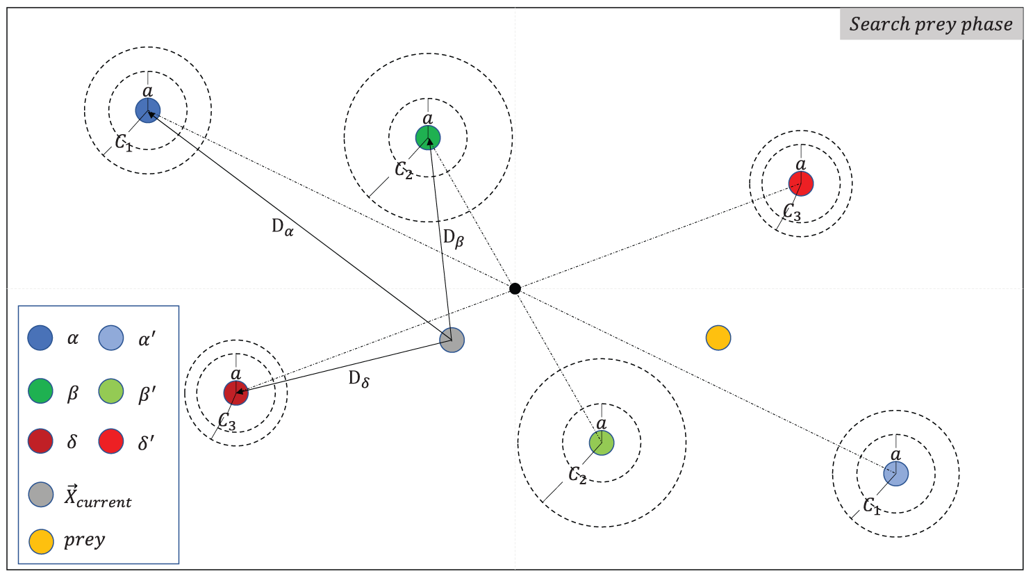
Figure 2: Add SW in the phase of searching prey

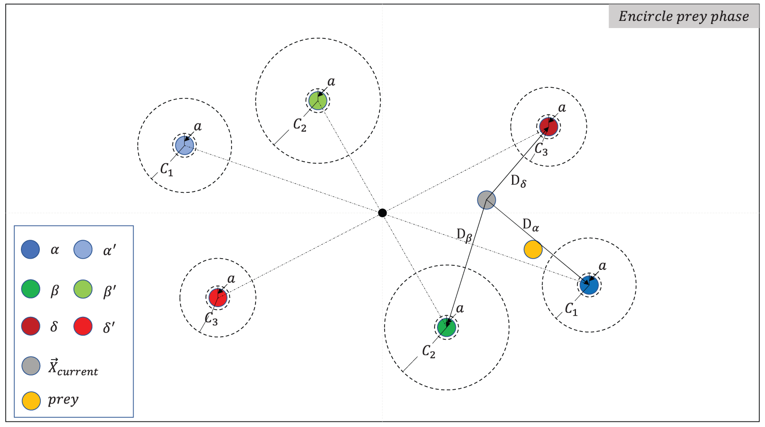
Figure 3: Add SW in the phase of encircling prey

For the SW wolves search in the iterative process, our study only searches for SW wolves for the first lengtℎ of well-fitness individuals in each iteration. This lengtℎ reduces linearly from N to 0 with the number of iterations. The computation formula is expressed as follows:

length=N∗Max_iter−itMax_iter,(1)

where N indicates the number of individuals in the population, it indicates the current iteration, and Max_iter indicates the number of iterations. This practice can prevent the time complexity of VGWO from becoming high.

3.2 Changing the Weights of α , β , and δ

As previously shown, changing the weight of the dominant wolf (i.e., α, β, and δ) can lead to better optimization capability [10], however, the weight of α should not always be greater than one-third. Although α is representative of the current optimal solution, it is not constantly closest to the prey [1]. If α always has the highest weight, then the wolves will inevitably gather around α prematurely, thereby ignoring the leadership of β and δ, and making the search easier to fall into the local optimum. Therefore, this paper proposes a new weight calculation method.

{ω1=23∗itMax_iterω2=13ω3=23−ω1,(2)

where ω1, ω2, and ω3 indicate the weight of α, β, and δ, respectively. ω1 linearly increases from 0 to 2/3 with the iterations it. ω2 indicates the weight of the individual in the middle position, and this paper simply keeps its weight to 1/3. ω3 linearly reduces from 2/3 to 0 with the number of iterations. As shown in Eq. (2), this calculation method aims to weaken the weight of α in the searching and encircling phases and strengthen the leadership of β and δ, thereby improving the global search ability and reducing the probability of wolves falling into the local optimum.

3.3 Adding Random Perturbations to Wolves

Random perturbation is a type of contingent fluctuation that can be used to test the stability and usefulness of a model [35]. Simulated annealing (SA) jumps out of local optimum by implementing a survival of the fittest strategy for random perturbations [36] like the greedy strategy proposed in DE [37]. On this basis, SA and DE have powerful random search capabilities. Contrary to GWO, the authors in [38] and [39] pointed out that SA and DE often need to pay the price of slow convergence speed. Therefore, this paper combines the advantages of the above three algorithms to create the VGWO, that is, adding random perturbations to the wolves. The random perturbations are generated as follows:

X→variation=X→r1+F∗(X→r2−X→r3),(3)

where r1, r2, and r3 are three different random integers in the range of [1, N], and F is the scaling parameter. In the DE, F affects the diversity of the population and has a remarkable effect on convergence and stability. The appropriate F is difficult to be determined. As mentioned in [40], the upper limit of F = 1.2 is determined on the basis of experience, and no optimization problem requires F to be greater than 1.2. Therefore, for wolves, after ending each search, creating the variant individuals with different F is a reasonable means to balance the local search and global search capabilities of the algorithm. For the VGWO, the value of F is linearly reduced from 1.2 to 0. This paper changes F in accordance with a special parameter, which is called temperature changing in SA.

F=1.2−1.2∗(Tmax−T)Tmax−Tmin(4)

where Tmax indicates the initial temperature, T indicates the temperature under the current iteration, and Tmin indicates the temperature under steady state. However, the judgment of whether a random perturbation is added to the wolf pack needs to be based on its fitness value.

A method for calculating the probability of a random perturbation being selected is proposed in the archival multiobjective SA algorithm (AMOSA) [41].

Probability=11+eΔdomavg∗T,(5)

where Δdomavg is the average domination of the random perturbation. T denotes the present temperature, and the above formula guarantees that the probability value is between 0 and 1. Δdomavg is determined as the following:

Δdomavg=(∑i=1k⁡Δdomi,b)/k,(6)

where k is the number of solutions, and Δdomi,b is the amount of domination about two solutions (i.e., i and b), which is determined by

Δdomi,b=∏j=1,fj(i)≠fj(b)O⁡(|fj(i)−fj(b)|/Rj)(7)

where the O is the number of objectives. In [41], the new solution is obtained by making a random perturbation to the current state, which is similar to the idea of deriving the variant individual in Eq. (3). However, the calculation of the average dominance in the AMOSA is based on a multiobjective problem, and the problem discussed in this study is a single-objective problem. In other words, O in Eq. (7) is equal to 1, and Eq. (6) represents the average domination of the new solution b over all the solutions. This strategy is similar to the vector 1-norm. The traditional vector 1-norm calculation method is as follows: ||x||1=∑i=1N|xi|, where x denotes an N-dimensional vector. The mathematical meaning of the 1-norm is the sum of the elements of a 1D vector, and the geometric meaning is the Manhattan distance from the vector x to the original point.

The Manhattan distance is a scalar that reflects the absolute value of the sum of the axial distances between two points. As shown in Fig. 4, the Manhattan distance of point x (1,1) to point y (4,5) is 7. However, this study wants to calculate the superiority or inferiority of variant individuals relative to the population as a whole in terms of fitness. Thus, a new method of calculating the Manhattan distance is needed to represent the above problem by the positive or negative of the Manhattan distance. This paper defines this method as the vectorized Manhattan distance to calculate the domination deviation of the variant wolf to the current population. In our study, the fitness value of the population is considered an N-dimensional vector, Fit→ = (Fitness (X→1), Fitness (X→2),..., Fitness (X→N)). Thus, the corresponding vectorized Manhattan distance calculation is expressed as

Vma→=[Fitness(X→variation),⋯]⏞N−Fit→,(8)

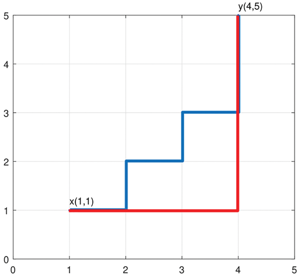
Figure 4: Manhattan distance from point x to point y (both the red and blue lines are Manhattan distances)

then we calculate the 1-norm M of non-absolute values of the Vma→ vector as the following:

M=∑i=1N⁡Vma[i](9)

where the Fitness() function is denoted as the fitness function. For example, X→variation is better than most individuals in the current wolves when the optimization objective of the fitness function is the minimum, and the value of M is less than 0. Thus, the vectorized Manhattan distance can be used to determine the status of random perturbations in the current population by the positive or negative of M. The pseudo-code for vectorized Manhattan distance calculation is presented in Algorithm 2.

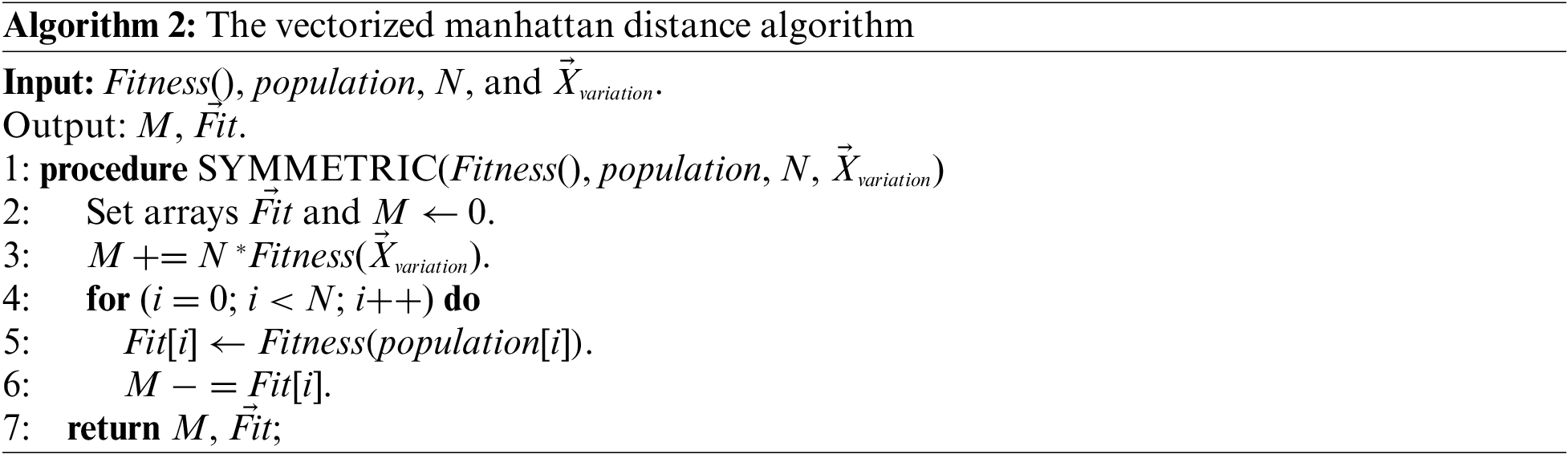
Combined with Eqs. (5) and (6), this paper can derive a new method for calculating the probability of a variation individual being selected is presented as follows:

P=11+eΔdomavg∗T=11+e(∑i=1kΔdomi,s)/k∗T=11+eMN∗T(10)

where N indicates the population number and T indicates the current temperature.

To better clarify the definition of variables, we list the variables used in this paper and give their corresponding descriptions in Table 1.

3.4 VGWO Process

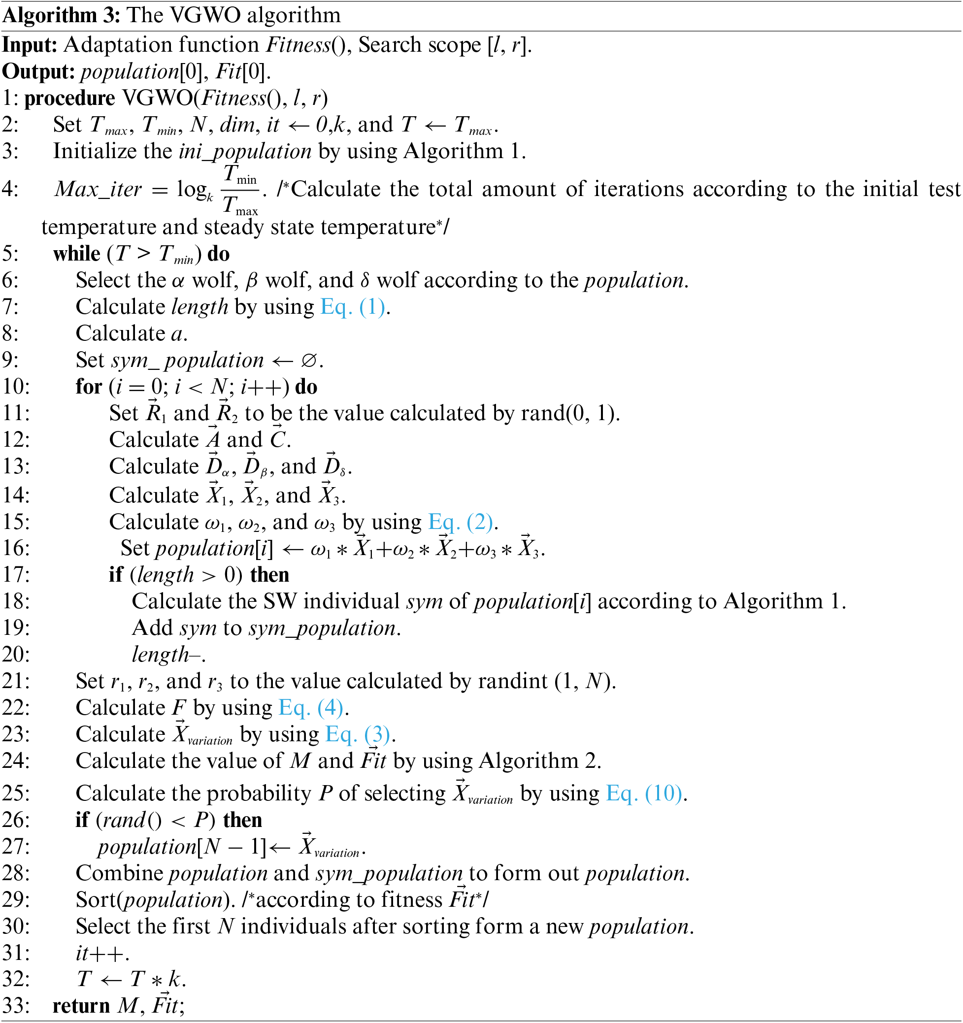
Algorithm 3 demonstrates the VGWO pseudo-code. The initialization section must determine the initial temperature Tmax, steady state temperature Tmin, and temperature change rate k based on the actual problem. The initialized population ini_population is generated on the basis of the population size and shape; the initialized individuals follow the beta distribution. The SW population sym_population is generated by using the method described in Section 3.1, ini_population and sym_population are merged to obtain population, and population is sorted by the fitness value. The top N individuals are chosen to form the final initial population. The total number of iterations Max_iter is calculated.

The second part is the process of slow cooling. Three wolves with the highest status in the wolves are selected as α, β, and δ. In accordance with Eq. (1), the number of SW wolves to be searched in each iteration (length) is calculated. sym_population is initialized as an empty set, which is used to save the SW of the first length wolves. The search process of grey wolves is the same as the original GWO. With the gradual decrease in length, the SW of the current grey wolf is searched after determining its new coordinates and saved in sym_population until length decreases to 0. Whenever the wolves have finished searching, the variation factor F is calculated by using Eq. (4). The variation is obtained as a new individual X→variation by using Eq. (3), and the domination M of X→variation is calculated in accordance with Algorithm 2. The probability of selecting X→variation is calculated by using Eq. (10). New offspring population and sym_population are combined, and the first N grey wolves are taken as the new population.

3.5 Complexity Analysis

Unlike the original GWO, the VGWO uses the quick sort to update the population with a time complexity of O(n ∗ log2n). Assume the time complexity of the fitness value calculation is set to T. The length of the population after the merging of the population and the sym_population is denoted by L, and the value of L reduces linearly from (2 ∗ N) to N with the number of iterations to facilitate the expression of the subsequent complexity. The basic operations’ complexities are as follows. 1) Initializing the wolves: O(N ∗ dim + 2 ∗ N ∗ log22 ∗ N); 2) Wolf searching: The number of iterations is Max_iter. The time complexity of updating the coordinates of wolves is O(N ∗ dim). The time complexity of calculating the vectorized Manhattan distance and fitness values is O(N ∗ T), while updating the population is O(L ∗ log2L). Therefore, the overall complexity of VGWO is O(Max_iter ∗ (N ∗ dim)).

The GWO, PSOGWO, and VWGWO all have the same time complexity, which is O(Max_iter ∗ (N ∗ dim)) [1,10,11]. The time complexity of the CMAGWO is O(iter1 ∗ (N ∗ dim)) + O((Max_iter − iter1) ∗ dim) [12], where iter1 denotes the number of iterations of the first stage in the CMAGWO. The time complexity difference between the five algorithms is small, and subtle differences may be observed. Thus, the effect on the performance of the algorithms is negligible in this study.

4  Experimental Settings

With the purpose of assessing the capability of the VGWO, we conduct a series of experiments. The algorithms being compared include GWO, VWGWO, PSOGWO, and CMAGWO. This section outlines the experimental steps and parameter setting. The experimental framework and programs used for comparison were implemented in Python and ran on a computer with a 2.90 GHz Intel i7-10700 CPU and 16 GB of RAM. The source code and experimental results are available at https://github.com/ZhifangSun/VGWO.

4.1 Benchmark Function

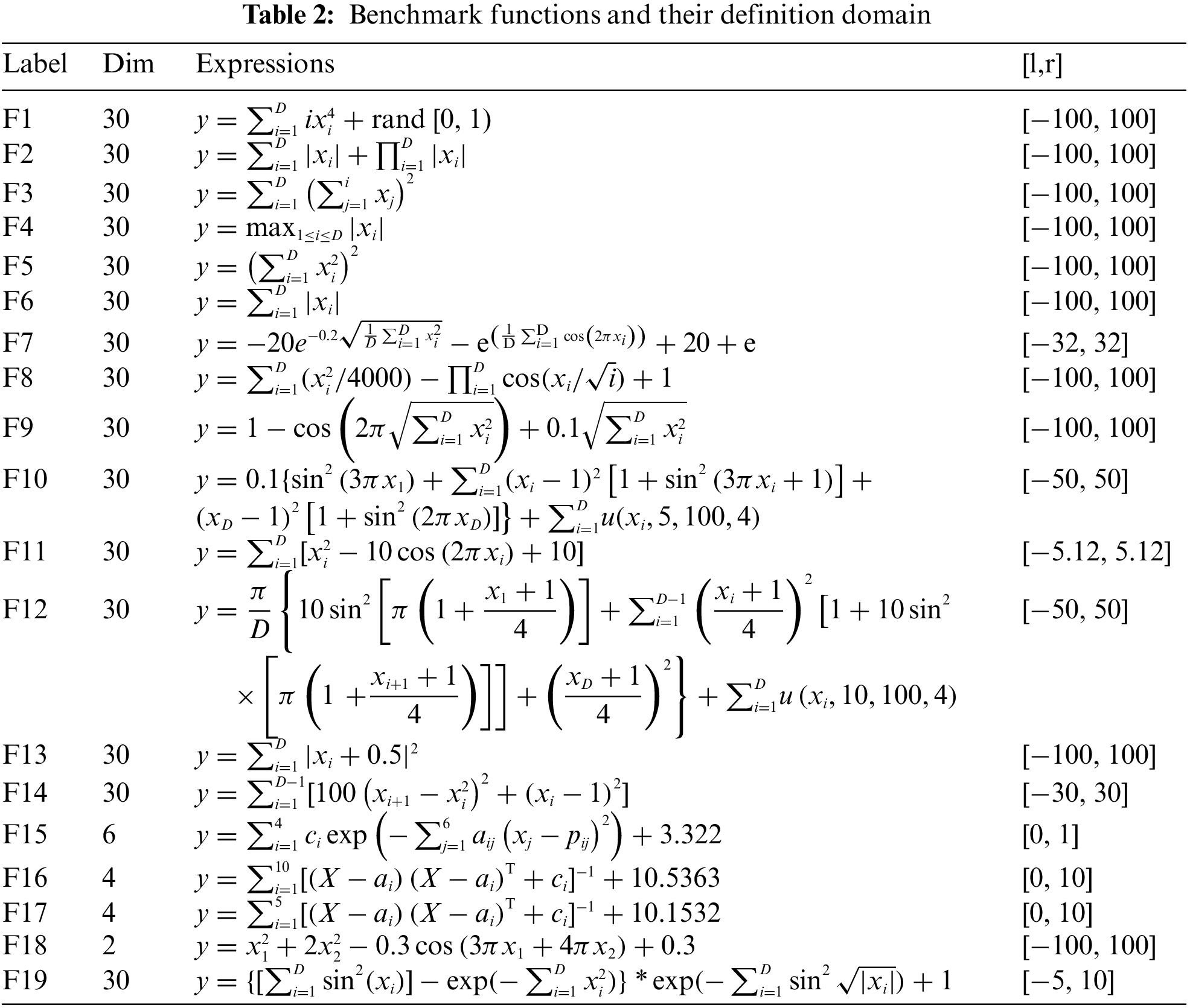
Benchmark function is a variety of standard functions derived from the optimization problems encountered by human beings in real life. This paper selected 19 representative benchmark functions from CEC2014 and CEC2020 to test the performance of the above algorithms, which are well-known complex test functions [42]. They can be divided into three main categories, namely, unimodal (F1, F2, F3, F4, F5, F6, F13, F14), multimodal (F7, F8, F9, F10, F11, F12, F19), and fixed-dimension multimodal (F15, F16, F17, F18). As shown in Table 2, the input D-dimensional vector X→ = (x1, x2, ···, xD) is limited by different definition fields. The maximum value and the minimum value in the definition field are r and l, respectively, and the optimum of each function is 0. For each tested algorithm, different random populations are used for 15 repeated tests, and the average solutions and standard deviations of all experiments are recorded.

4.2 Parameter Setting of VGWO

Orthogonal experimental design is a multi-factor, multi-level experimental design method [43], which is fast, economical, and efficient, and can obtain satisfactory results with a fewer number of experiments. Therefore, the orthogonal test method is often used to compare the nature of parameters and to determine the best combination between different parameters. The parameters that need to be set in advance for this experiment are the rate of temperature change k, the starting temperature Tmax, and the steady state temperature Tmin. The three parameters control the global number of iterations Max_iter, the variation factor F, and the admission probability P of the perturbed individuals. Therefore, different combinations and different levels of the 3 parameters are shown in Table 3.

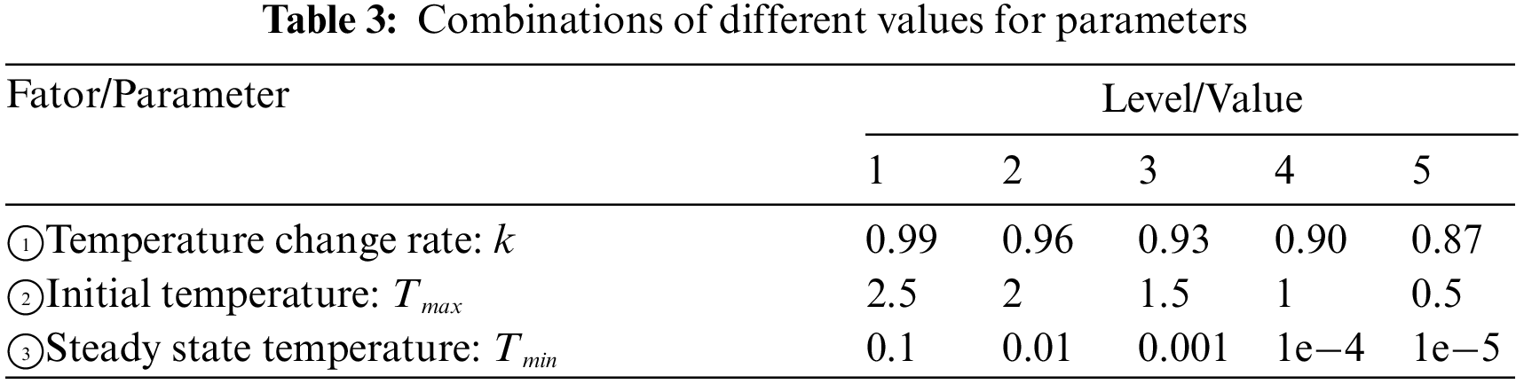
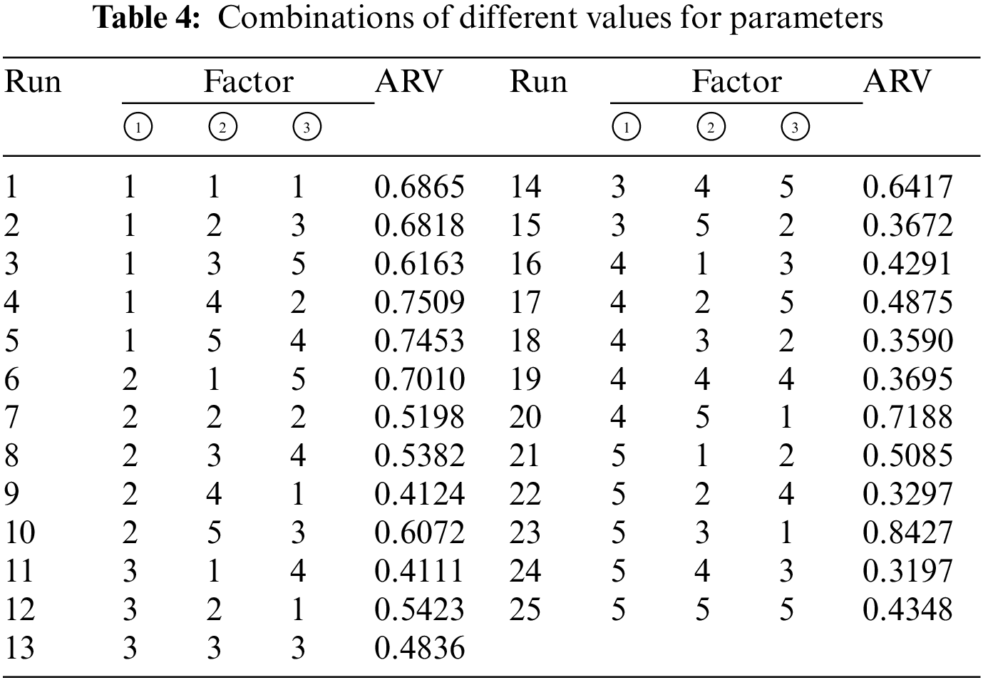
Table 3 lists factors/parameters and their corresponding levels/values. The number of orthogonal groups of L25(53) was chosen for this experiment. For each set of orthogonal experiments, five tests are performed, and the test termination condition is when the scheduling time of the VGWO reaches stla = max {astGWOla,astVWGWOla,astPSOGWOla,astCMAGWOla}, where astalgorithmla denotes the average scheduling time of the la-th benchmark function after 300 iterations through algorithm, where algorithm ∈ {GWO, VWGWO, PSOGWO, CMAGWO}, and la ∈ Label, for the benchmark functions in Table 2. The results of the orthogonal experiments are shown in the GitHub repository mentioned in Section 4.

The performance of the GWOs is linked to the parameter values when faced with different problems, and a tuned combination of parameter values will yield better results. However, the experiments use the same combination of parameters to optimize different benchmark functions for highlighting the performance of VGWO. Thus, the average response value (ARV) of the i-th parameter combination is calculated by using the following equation:

ARVi=15|Label|∑j=15∑la∈Label{ansi,jla−mini=1,⋯,25;j=1,⋯,5{ansla}}(11)

where ansi,jla represents the VGWO optimized result of the la-th benchmark function of the j-th when selecting the i-th set of parameter combinations, and the value of ARV can reflect the performance of each of the 25 sets of parameter combinations.

The ARVs obtained from the orthogonal experiments are shown in Table 4. Table 5 shows the mean value of ARV and the extreme difference in the mean value for each factor at different levels. A smaller value of ARV indicates that this parameter has less difference from the global optimum at the current level, and a larger value of ARV indicates that this parameter has less optimization ability at the current level. The larger the extreme difference in the mean value of ARV indicates that this parameter has more influence on the performance of the algorithm. Therefore, the conclusions based on Tables 4 and 5 are summarized as follows:

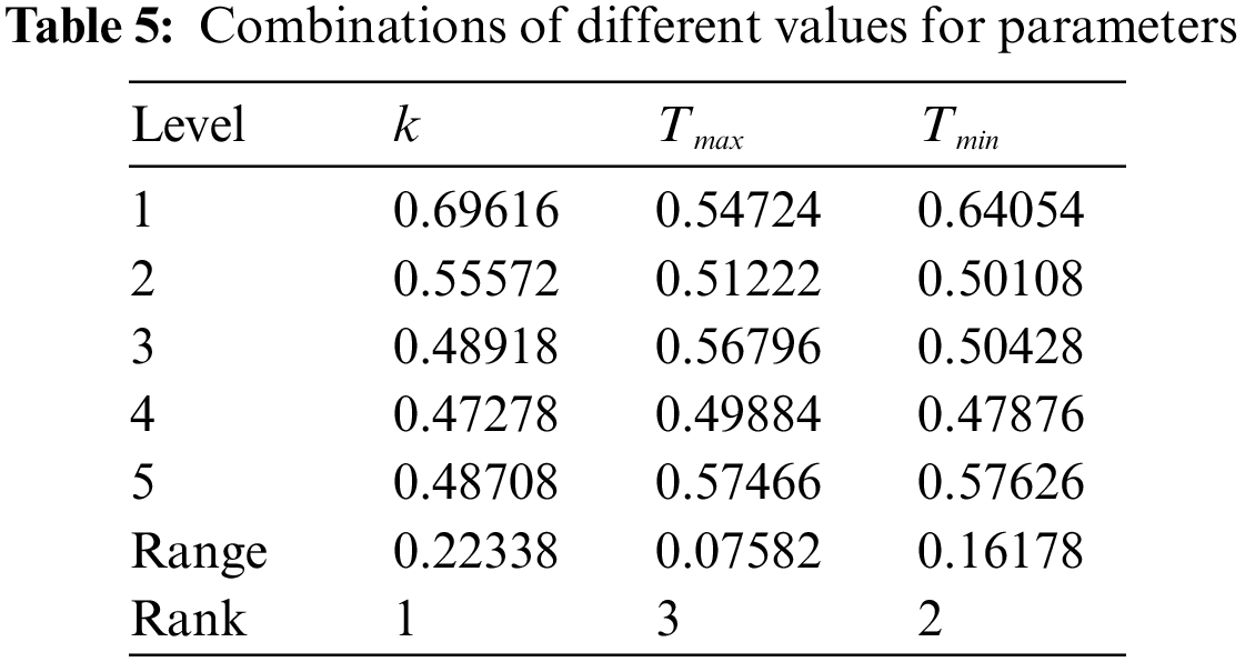
1.    In accordance with the value of range, the effect of the three parameters on the performance of the algorithm from low to high is Tmax, Tmin, k.

2.    Based on each factor’s mean ARV value of different levels, the best combination of parameters for the VGWO is suggested to be Tmax = 1, Tmin = 1e−4, and k = 0.90.

3.    The extreme differences of all three parameters are small, less than 0.25, which shows that the algorithm is not sensitive to the values of the parameters, and has robust and stable performance within a wide range of parameter settings.

4.3 Other Parameter Settings

The parameters of the VGWO are obtained in Section 4.2 (i.e., Tmax = 1, Tmin = 1e−4, and k = 0.90), and the parameters of the remaining algorithms (GWO [1], PSOGWO [11], VWGWO [10], CMAGWO [12]) are set in the same way as the parameters of the respective references. The number of iterations of all algorithms is 90, and the number of wolves is 50.

5  Experimental Result

This section presents and discusses the results of the proposed VGWO compared with the state-of-art GWOs. Mainly comparing their performance through optimization results and convergence curves.

5.1 Result Analysis

The optimal solutions of the above 10 functions and the algorithms that produce this result are recorded in Table 6, where the optimal average solution of each function is marked in boldface. Given that the generation of the wolves is random and has certain instability in the iterative process, the results that are different from the ideal state exist. However, they are determined by the excellence of the algorithm itself in most cases.

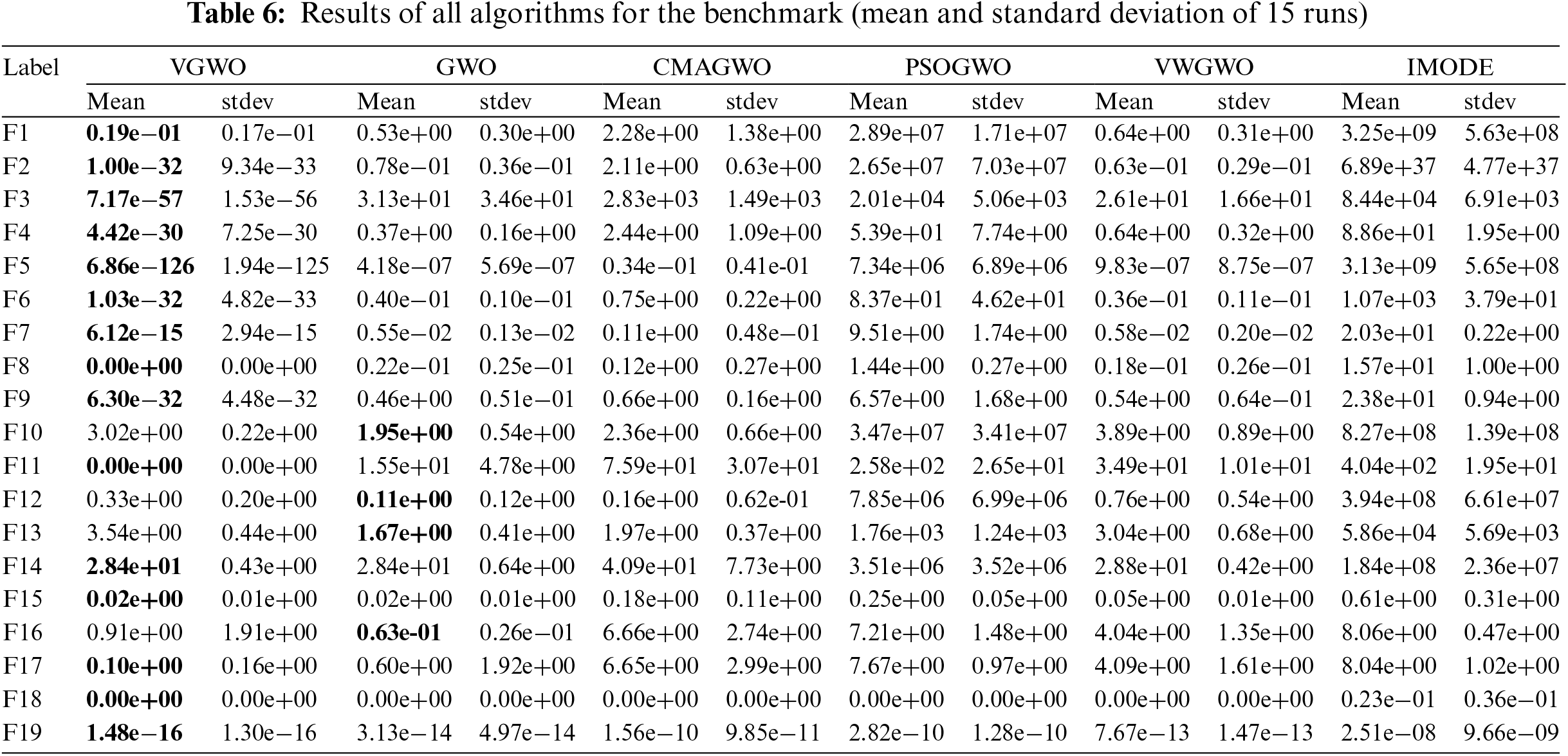
The results of the 19 benchmark functions are analyzed as follows:

1)   For all functions, most of the optimal average solutions compared with various algorithms are found by the VGWO. Because the VGWO enhances the diversity of wolves through SW, it outperforms other algorithms in terms of finding the best solution and even produces the ideal solution 0 for functions F8, F11, and F18. In each iteration, VGWO will arrange more ω wolves to search for prey, which greatly increases the probability of obtaining the global optimum.

2)   The standard deviation of F8, F11, and F18 functions is 0, and the other four GWOs easily fall into local optimum, so it is difficult to achieve this level. VGWO generates random perturbations through differential operators, and calculates the probability of acceptance through its own domination. This method provides a chance for the stability of the wolves to jump out of the local optimum, which reflects the strong robustness of VGWO.

3)   F10 and F12 are multi-peaked functions, F13 is a single-peaked function, and F16 is a fixed-dimensional multi-peaked function. Although the GWO achieves the lead, it does not differ much from the results obtained by the VGWO, and VGWO has good performance for other functions of the same type.

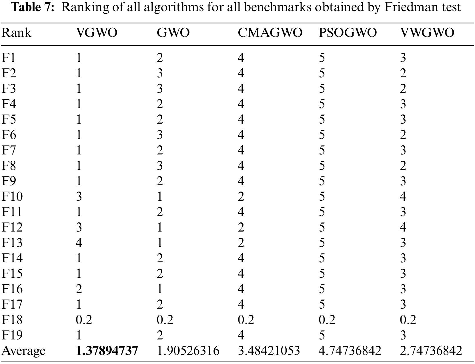
In addition, the Friedman test results shown in Table 7 indicate that VGWO ranks first in terms of average results. It is clear that VGWO is statistically superior to all other algorithms since it has an average ranking value.

5.2 Convergence Curve Analysis

Figs. 5–7 show most of the fitness value iteration plots. The rest of the functions not shown are due to either excessive disparity or similarities in the convergence curves between different algorithms. GWOs’ excellence cannot be compared visually by the graphs. Considering that the curves of different GWOs overlap in these graphs, some iteration graphs have additional small views, which can be used to visualize the distribution of the overlapping curves at the end of the iteration.

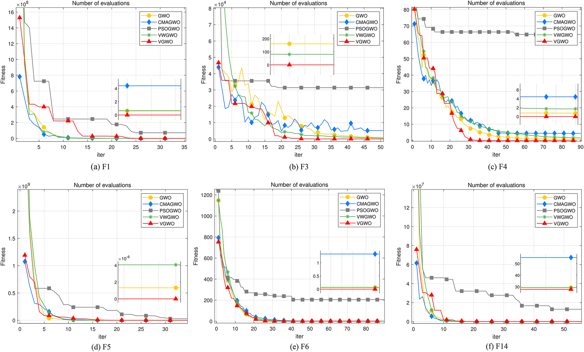
Figure 5: Unimodal benchmark functions

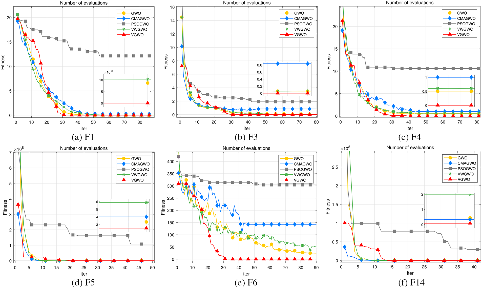
Figure 6: Multimodal benchmark functions

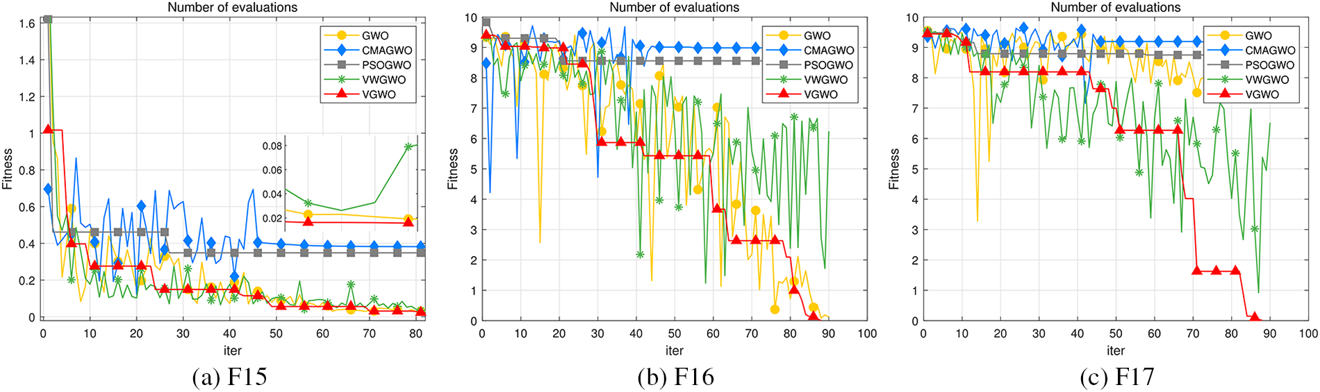
Figure 7: Fixed-dimension multimodal benchmark functions

The analysis results for the three different types of benchmark functions (unimodal, multimodal, and fixed-dimension multimodal benchmark functions) are as follows:

1)   For the unimodal benchmark function, the VGWO and CMAGWOs have excellent capabilities in initializing populations due to the beta distribution. Figs. 5b and 5c show that the convergence rate at the beginning is still slow. This finding is due to the improved mechanism proposed in Section 3 enhances the population diversity of the pre-VGWO. However, this scheme does not affect the convergence speed of the VGWO, and the rich population diversity enhances the convergence speed of the VGWO in the later stages. As shown in Figs. 5b and 5c, for the above reasons, the VGWO obtains a solution that exceeds the rest of the algorithms when the number of iterations reaches about the 20th time.

2)   For the multimodal benchmark function, except for the PSOGWO that will fall into the local optimum prematurely, the rest of the algorithms have a good convergence trend, where the most outstanding performance is still the VGWO. With the continuous addition of random perturbations, and accepting wolves with dominant positions, the VGWO can jump out of the local optimum easily and establish the search area quickly by the rich population diversity.

3)   For the fixed-dimension multimodal benchmark function, many algorithms fall into local optimum, and the curves of the GWO, VWGWO, and VGWO show a decreasing trend, as shown in Fig. 7a. In Fig. 7b, only the GWO and the VGWO converge toward the amiable results. In Fig. 7c, only the VGWO converges to the ideal results. The GWO, CMAGWO, PSOGWO, and VWGWO are difficult to determine the approximate position of the prey and present extremely unstable curves. This is due to VGWO's guarantee of population diversity, which reflects the strong robustness of the VGWO.

5.3 Comparison with CEC Competition Winner

To judge the performance of VGWO further, this study compares the results obtained by VGWO from the 19 benchmark functions mentioned above with those obtained by the winner of the CEC2020 competition, an improved multi-operator DE (IMODE) algorithm. Its parameters are obtained from relevant articles, and the same random seeds are used for both VGWO and IMODE to ensure a fair comparison.

The mean and standard deviation of the results are recorded according to the rules of the benchmark.

The run was stopped if the number of evolutions was greater than 90. The performance comparison between VGWO and IMODE is shown in Table 6.

By the mean and standard deviation obtained, the proposed VGWO outperforms IMODE for unimodal, multimodal, and fixed-dimension multimodal problems. In [44], IMODE obtains good results by a large number of iterations and running time. However, in this study, the results obtained by IMODE are much worse compared to VGWO. This shows that VGWO is able to obtain better results after fewer iterations compared to IMODE, proving that VGWO has higher accuracy and convergence.

6  Application Studies on Engineering Cases

Engineering examples are designed in such a way that the solution usually involves constraints on inequalities or equations. The methods to handle the constraints are special operators, repair algorithms, and penalty functions [45]. The simplest method is used because this study ignores additional algorithms for the VGWO to design good handling of constraints. In simple terms, any solutions that violate the constraints are uniformly penalized by assigning them the maximum fitness value (minimum fitness value in the maximization case). This method is extremely easy to implement and requires no modification to the VGWO.

In the following summary, the VGWO will be used to solve 3 constrained engineering problems and each engineering case will be run 15 times to compare the optimization results with the GWO, CMAGWO, PSOGWO, and VWGWO. The number of iterations of all algorithms is 90, and the number of wolves is 50. The parameter settings for all algorithms are the same as in Section 4.

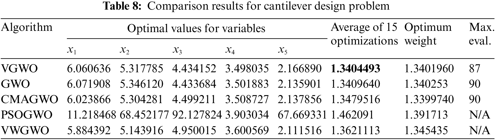
6.1 Cantilever Beam Design Problem

Fig. 8 shows the model of a cantilever beam, which consists of five hollow elements of a square cross section, each corresponding to a variable parameter. From Fig. 8, the right side of element 1 is rigidly supported, and element 5 is subjected to a vertical load [46]. The optimization objective is to minimize the total weight of the beam without violating the vertical displacement constraint. The weight of the beam is calculated by using the following formula:

f(x→)=0.0624∗(x1+x2+x3+x4+x5)(12)

Figure 8: Cantilever beam design problem

The constraint function for the vertical displacement can be expressed as follows:

g(x→)=61x13+37x23+19x33+7x43+1x53≤1(13)

where 0.01 ≤ x1, x2, x3, x4, x5 ≤ 100. Table 8 shows the best results of the five algorithms optimized for this engineering example. The VGWO achieves the best average result after 15 iterations of the experiment. Although the global optimal solution is obtained by the CMAGWO, its average result is inferior to that of the VGWO, which reflects the stability of the VGWO. The last column of the table (Max. eval.) represents the maximum number of evaluations required for the algorithm of this row to converge to the average value of the VGWO (bolded values in the table), and N/A represents the inability to reach the average of the VGWO. This finding shows that the VGWO only requires a smaller number of evaluations to converge to a better solution, reflecting the higher accuracy of the results obtained by VGWO.

6.2 Three-Bar Truss Design Problem

Fig. 9 shows the second engineering example, which is the design of a threebar truss with the optimization objective of minimizing its weight while being constrained by buckling and stresses [47], where trusses x1 and x3 are the same. The objective function can be expressed as

f(x→)=(22x1+x2)∗l(14)

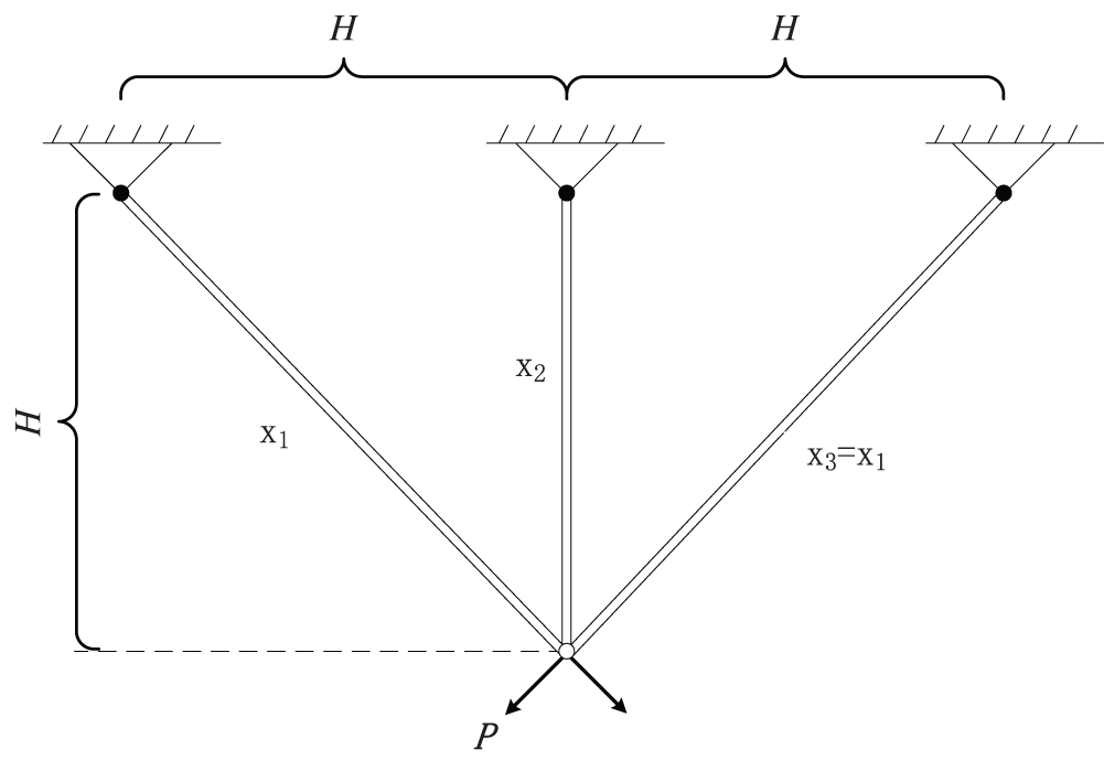
Figure 9: Three-bar truss design problem

The constraint function can be expressed as

{g(x→)=2x1+x22x12+2x1x2P−σ≤0g(x→)=x22x12+2x1x2P−σ≤0g(x→)=12x2+x1P−σ≤0,(15)

where 0 ≤ x1, x2 ≤ 1, l = 100 cm, P = 2 kN/cm2, σ = 2 kN/cm2. From Table 9, the VGWO achieves the optimal average result, obtains the global optimal solution among the five algorithms, and only uses 79 iterations. The optimal solutions obtained by GWO, PSOGWO, and VWGWO are less than the average of VGWO, which again proves the efficiency of the VGWO in solving engineering instance problems.

6.3 Gear Train Design Problem

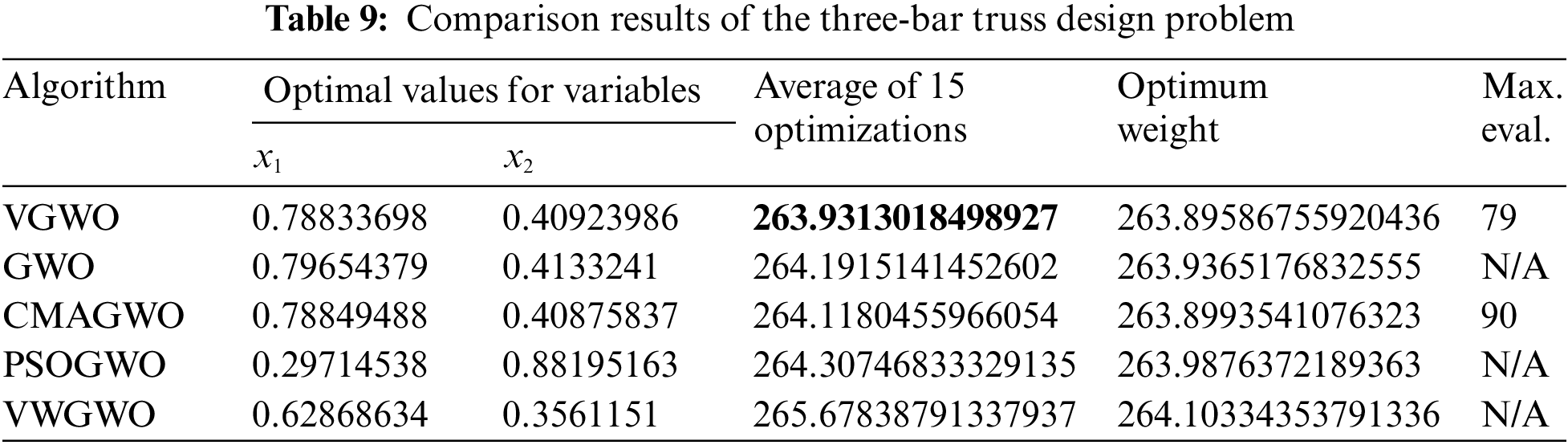
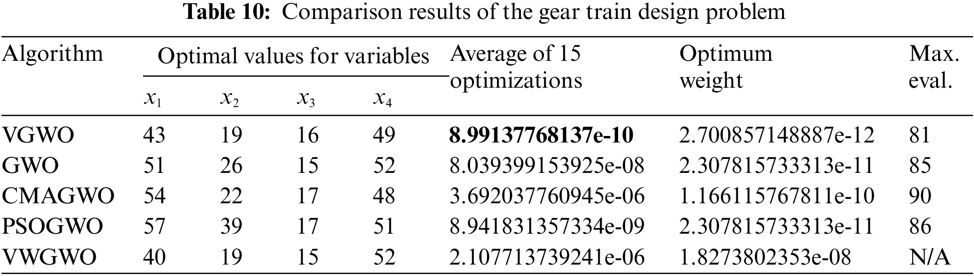
Fig. 10 shows the third engineering example, which is a discrete case study with four parameters representing four gears (i.e., A, B, C, and D), and the optimization objective is to minimize the rotation ratio of the gears and determine the optimal number of teeth for the four gears at this time [48]. The objective function can be expressed as follows:

f(x→)=(16.931−x2x3x1x4)2(16)

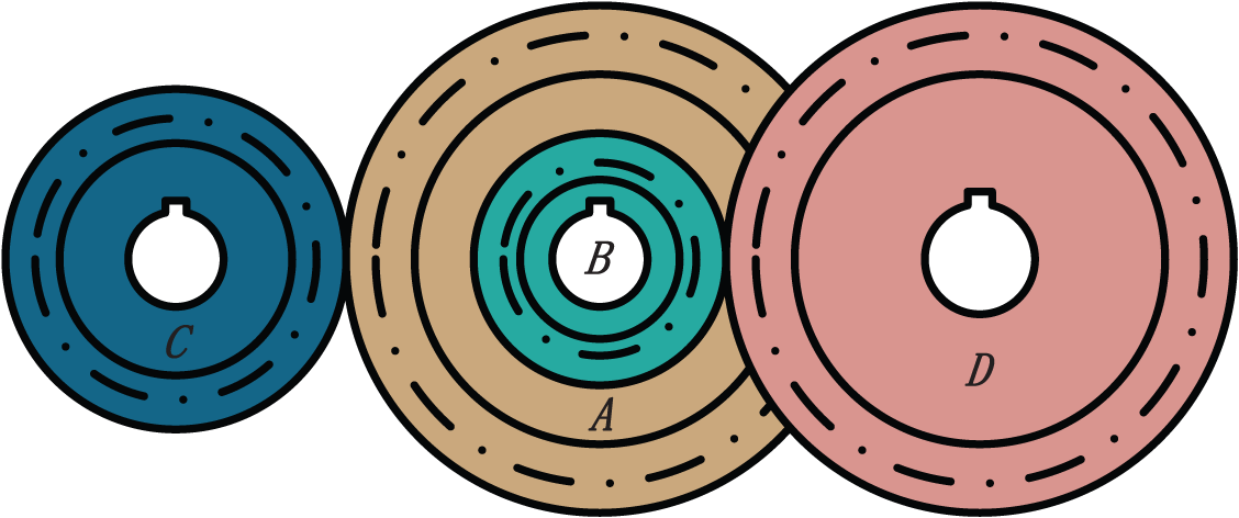
Figure 10: Gear train design problem

Its constraints are relatively simple and only need to be satisfied as follows: 12 ≤ x1, x2, x3, x4 ≤ 60. According to [49], when the optimal number of teeth is set to x1 = 43, x2 = 19, x3 = 16, and x4 = 49, then the gear rotation ratio will obtain the smallest value. As shown in Table 10, VGWO obtains this result by only through 81 iterations, and its average result is the best among the five algorithms. From the above three engineering examples, the VGWO is suitable for most of optimization problems with constraints and can obtain better results after relatively fewer iterations, which reflects the robustness, stability, and strong convergence of the VGWO.

7  Conclusion

In this study, this paper proposes a high-accuracy VGWO while still with low time complexity. SW is used to enhance the diversity of the wolves. Inspired by VWGWO’s proposal that three dominant grey wolves have different social statuses in different periods, this study improves the linear variation method of the three dominant wolves’ weights during the search procedure. With the purpose of reducing the chance of falling under local optimum, a differential variation factor is introduced to generate new individuals. Enlightened by the AMOSA, the probability of accepting the random perturbation is calculated by vectorizing the Manhattan distance when the grey wolf finishes the current search. The experimental comparison of 19 benchmark functions, the CEC competition winner (IMODE), and 3 engineering cases with GWO, CMAGWO, PSOGWO, and VWGWO reflects the advantages of VGWO in terms of convergence and accuracy. The experimental results show that our VGWO has better solution quality and robustness than other algorithms under different conditions. For 19 benchmark functions, VGWO's optimization results place first in 80% of comparisons to the state-of-art GWOs and the CEC2020 competition winner. Only VGWO's average ranking value is less than 1.5, according to Friedman's test.

The proposed VGWO is promising to be a good choice for solving problems with uncertain search ranges and high requirements for accuracy of results. However, the proposed improvements mainly focus on increasing the wolves’ diversity, which is not necessarily applicable to solve all benchmark functions. Tendency to fall into local optimum is still a weakness of the GWO. VGWO is not always the best solution when encountering a larger range of solution spaces than the current popular application problem, and further efforts are needed to solve this problem. The GWO is still a hot topic for future research on optimization algorithms, and the application of VGWO to suitable engineering optimization problems will be considered in the future. For example, it can be applied to renewable energy systems, to workflow scheduling problems in heterogeneous distributed computing systems, or to integrated process planning and scheduling problems. As more excellent intelligent optimization algorithms are proposed, we will try to shift our research direction to these algorithms in the future, such as Mountain Gazelle Optimizer [50], African Vultures Optimization Algorithm [51], and so on.

Acknowledgement: We would like to thank the anonymous reviewers for their valuable comments on improving the paper.

Funding Statement: This work is partially funded by the China Scholarship Council.

Author Contributions: Study conception and design: Junqiang Jiang, Zhifang Sun; data collection: Xiong Jiang; analysis and interpretation of results: Shengjie Jin, Yinli Jiang; draft manuscript preparation: Junqiang Jiang, Zhifang Sun, Bo Fan. All authors reviewed the results and approved the final version of the manuscript.

Availability of Data and Materials: The authors confirm that the data supporting the findings of this study are available within the article.

Conflicts of Interest: The authors declare that they have no conflicts of interest to report regarding the present study.

References

1. S. Mirjalili, S. M. Mirjalili and A. Lewis, “Grey wolf optimizer,” Advances in Engineering Software, vol. 69, pp. 46–61, 2014. [Google Scholar]

2. A. Faramarzi, M. Heidarinejad, B. Stephens and S. Mirjalili, “Equilibrium optimizer: A novel optimization algorithm,” Knowledge-Based Systems, vol. 191, pp. 105190, 2020. [Google Scholar]

3. W. Zhao, L. Wang and S. Mirjalili, “Artificial hummingbird algorithm: A new bio-inspired optimizer with its engineering applications,” Computer Methods in Applied Mechanics and Engineering, vol. 388, no. 1, pp. 114194, 2022. [Google Scholar]

4. M. H. Nadimi-Shahraki, S. Taghian, H. Zamani, S. Mirjalili and M. A. Elaziz, “MMKE: Multi-trial vector-based monkey king evolution algorithm and its applications for engineering optimization problems,” PLoS One, vol. 18, no. 1, pp. e0280006, 2023. [Google Scholar] [PubMed]

5. H. R. R. Zaman and F. S. Gharehchopogh, “An improved particle swarm optimization with backtracking search optimization algorithm for solving continuous optimization problems,” Engineering with Computers, vol. 38, no. Suppl 4, pp. 2797–2831, 2022. [Google Scholar]

6. Y. Shen, C. Zhang, F. S. Gharehchopogh and S. Mirjalili, “An improved whale optimization algorithm based on multi-population evolution for global optimization and engineering design problems,” Expert Systems with Applications, vol. 215, pp. 119269, 2023. [Google Scholar]

7. G. Komaki and V. Kayvanfar, “Grey wolf optimizer algorithm for the two-stage assembly flow shop scheduling problem with release time,” Journal of Computational Science, vol. 8, no. 22, pp. 109–120, 2015. [Google Scholar]

8. X. Song, L. Tang, S. Zhao, X. Zhang, L. Li et al., “Grey wolf optimizer for parameter estimation in surface waves,” Soil Dynamics and Earthquake Engineering, vol. 75, no. 3, pp. 147–157, 2015. [Google Scholar]

9. H. S. Suresha and S. S. Parthasarathy, “Detection of Alzheimer’s disease using grey wolf optimization based clustering algorithm and deep neural network from magnetic resonance images,” Distributed and Parallel Databases, vol. 40, no. 4, pp. 627–655, 2022. [Google Scholar]

10. Z. M. Gao and J. Zhao, “An improved grey wolf optimization algorithm with variable weights,” Computational Intelligence and Neuroscience, vol. 2019, pp. 2981282, 2019. [Google Scholar] [PubMed]

11. Z. J. Teng, J. L. Lv and L. W. Guo, “An improved hybrid grey wolf optimization algorithm,” Soft Computing, vol. 23, no. 15, pp. 6617–6631, 2019. [Google Scholar]

12. Y. T. Zhao, W. G. Li and A. Liu, “Improved grey wolf optimization based on the two-stage search of hybrid CMA-ES,” Soft Computing, vol. 24, no. 2, pp. 1097–1115, 2020. [Google Scholar]

13. W. Long and T. Wu, “Improved grey wolf optimization algorithm coordinating the ability of exploration and exploitation,” Control and Decision, vol. 32, no. 10, pp. 1749–1757, 2017. [Google Scholar]

14. Q. Luo, S. Zhang, Z. Li and Y. Zhou, “A novel complex-valued encoding grey wolf optimization algorithm,” Algorithms, vol. 9, no. 1, pp. 4, 2015. [Google Scholar]

15. M. Kohli and S. Arora, “Chaotic grey wolf optimization algorithm for constrained optimization problems,” Journal of Computational Design and Engineering, vol. 5, no. 4, pp. 458–472, 2018. [Google Scholar]

16. S. Saremi, S. Z. Mirjalili and S. M. Mirjalili, “Evolutionary population dynamics and grey wolf optimizer,” Neural Computing and Applications, vol. 26, no. 5, pp. 1257–1263, 2015. [Google Scholar]

17. N. Mittal, U. Singh and B. S. Sohi, “Modified grey wolf optimizer for global engineering optimization,” Applied Computational Intelligence and Soft Computing, vol. 2016, pp. 7950348, 2016. [Google Scholar]

18. C. Lu, L. Gao and J. Yi, “Grey wolf optimizer with cellular topological structure,” Expert Systems with Applications, vol. 107, pp. 89–114, 2018. [Google Scholar]

19. P. Yao and H. Wang, “Three-dimensional path planning for UAV based on improved interfered fluid dynamical system and grey wolf optimizer,” Control and Decision, vol. 31, no. 4, pp. 701–708, 2016. [Google Scholar]

20. A. Zhu, C. Xu, Z. Li, J. Wu and Z. Liu, “Hybridizing grey wolf optimization with differential evolution for global optimization and test scheduling for 3D stacked soc,” Journal of Systems Engineering and Electronics, vol. 26, no. 2, pp. 317–328, 2015. [Google Scholar]

21. D. Jitkongchuen, “A hybrid differential evolution with grey wolf optimizer for continuous global optimization,” in 2015 7th Int. Conf. on Information Technology and Electrical Engineering (ICITEE), Chiang Mai, Thailand, IEEE, pp. 51–54, 2015. [Google Scholar]

22. X. Xia, L. Gui, F. Yu, H. Wu, B. Wei et al., “Triple archives particle swarm optimization,” IEEE Transactions on Cybernetics, vol. 50, no. 12, pp. 4862–4875, 2020. [Google Scholar] [PubMed]

23. N. Singh and S. Singh, “Hybrid algorithm of particle swarm optimization and grey wolf optimizer for improving convergence performance,” Journal of Applied Mathematics, vol. 2017, pp. 2030489, 2017. [Google Scholar]

24. A. Madadi and M. M.Mahmood, “Optimal control of DC motor using grey wolf optimizer algorithm,” Technical Journal of Engineering and Applied Sciences, vol. 4, no. 4, pp. 373–379, 2014. [Google Scholar]

25. D. K. Lal, A. K. Barisal and M. Tripathy, “Grey wolf optimizer algorithm based fuzzy PID controller for AGC of multi-area power system with TCPS,” Procedia Computer Science, vol. 92, no. 1, pp. 99–105, 2016. [Google Scholar]

26. A. H. Sweidan, N. El-Bendary, A. E. Hassanien, O. M. Hegazy and A. E. Mohamed, “Water quality classification approach based on bio-inspired gray wolf optimization,” in 7th Int. Conf. of Soft Computing and Pattern Recognition (SoCPaR), Fukuoka, Japan, IEEE, pp. 1–6, 2015. [Google Scholar]

27. S. Eswaramoorthy, N. Sivakumaran and S. Sankaranarayanan, “Grey wolf optimization based parameter selection for support vector machines,” COMPEL-The International Journal for Computation and Mathematics in Electrical and Electronic Engineering, vol. 35, no. 5, pp. 1513–1523, 2016. [Google Scholar]

28. N. Muangkote, K. Sunat and S. Chiewchanwattana, “An improved grey wolf optimizer for training q-Gaussian radial basis functional-link nets,” in Int. Computer Science and Engineering Conf. (ICSEC), Khon Kaen, Thailand, IEEE, pp. 209–214, 2014. [Google Scholar]

29. S. Mirjalili, “How effective is the Grey Wolf optimizer in training multi-layer perceptrons,” Applied Intelligence, vol. 43, no. 1, pp. 150–161, 2015. [Google Scholar]

30. A. Al-Shaikh, B. A. Mahafzah and M. Alshraideh, “Metaheuristic approach using grey wolf optimizer for finding strongly connected components in digraphs,” Journal of Theoretical and Applied Information Technology, vol. 97, no. 16, pp. 4439–4452, 2019. [Google Scholar]

31. G. Sivarajan, S. Subramanian, N. Jayakumar and E. B. Elanchezhian, “Dynamic economic dispatch for wind-combined heat and power systems using grey wolf optimization,” International Journal of Applied Mathematics and Computer Science, vol. 2, no. 3, pp. 24–32, 2015. [Google Scholar]

32. M. AlShabi, C. Ghenai, M. Bettayeb, F. F. Ahmad and M. E. H. Assad, “Multi-group grey wolf optimizer (MG-GWO) for estimating photovoltaic solar cell model,” Journal of Thermal Analysis and Calorimetry, vol. 144, no. 5, pp. 1655–1670, 2021. [Google Scholar]

33. A. A. Almazroi and M. M. Eltoukhy, “Grey wolf-based method for an implicit authentication of smartphone users,” Computers, Materials & Continua, vol. 75, no. 2, pp. 3729–3741, 2023. [Google Scholar]

34. H. G. Zaini, “Forecasting of appliances house in a low-energy depend on grey wolf optimizer,” Computers, Materials & Continua, vol. 71, no. 2, pp. 2303–2314, 2022. [Google Scholar]

35. A. V. Skorokhod, F. C. Hoppensteadt and H. D. Salehi, “Random perturbation methods with applications in science and engineering,” in Springer Science & Business Media, 1st ed., vol. 150. New York, USA: Springer, 2007. [Google Scholar]

36. S. Kirkpatrick, C. D. Gelatt and M. P. V. ecchi, “Optimization by simulated annealing,” Science, vol. 220, no. 4598, pp. 671–680, 1983. [Google Scholar] [PubMed]

37. R. Storn and K. Price, “Differential evolution-a simple and efficient heuristic for global optimization over continuous spaces,” Journal of Global Optimization, vol. 11, no. 4, pp. 341–359, 1997. [Google Scholar]

38. S. Zhou, L. Xing, X. Zheng, N. Du, L. Wang et al., “A selfadaptive differential evolution algorithm for scheduling a single batchprocessing machine with arbitrary job sizes and release times,” IEEE Transactions on Cybernetics, vol. 51, no. 3, pp. 1430–1442, 2019. [Google Scholar]

39. J. Bi, H. Yuan, S. Duanmu, M. Zhou and A. Abusorrah, “Energyoptimized partial computation offloading in mobile-edge computing with genetic simulated-annealing-based particle swarm optimization,” IEEE Internet of Things Journal, vol. 8, no. 5, pp. 3774–3785, 2020. [Google Scholar]

40. R. Mallipeddi, P. N. Suganthan, Q. K. Pan and M. F. Tasgetiren, “Differential evolution algorithm with ensemble of parameters and mutation strategies,” Applied Soft Computing, vol. 11, no. 2, pp. 1679–1696, 2011. [Google Scholar]

41. S. Bandyopadhyay, S. Saha, U. Maulik and K. Deb, “A simulated annealing-based multiobjective optimization algorithm: Amosa,” IEEE Transactions on Evolutionary Computation, vol. 12, no. 3, pp. 269–283, 2008. [Google Scholar]

42. J. J. Liang, B. Y. Qu and P. N. Suganthan, “Problem definitions and evaluation criteria for the CEC 2014 special session and competition on single objective real-parameter numerical optimization,” in Technical Report 201311. Singapore: Nanyang Technological University, vol. 635, no. 2, 2013. [Google Scholar]

43. Y. W. Leung and Y. Wang, “An orthogonal genetic algorithm with quantization for global numerical optimization,” IEEE Transactions on Evolutionary Computation, vol. 5, no. 1, pp. 41–53, 2001. [Google Scholar]

44. K. M. Sallam, S. M. Elsayed, R. K. Chakrabortty and M. J. Ryan, “Improved multi-operator differential evolution algorithm for solving unconstrained problems,” in 2020 IEEE Cong. on Evolutionary Computation (CEC), Glasgow, UK, IEEE, pp. 1–8, 2020. [Google Scholar]

45. J. Del Ser, E. Osaba, D. Molina, X. S. Yang, S. Salcedo-Sanz et al., “Bioinspired computation: Where we stand and what’s next,” Swarm and Evolutionary Computation, vol. 48, no. 1, pp. 220–250, 2019. [Google Scholar]

46. S. Li, H. Chen, M. Wang, A. A. Heidari and S. Mirjalili, “Slime mould algorithm: A new method for stochastic optimization,” Future Generation Computer Systems, vol. 111, pp. 300–323, 2020. [Google Scholar]

47. A. Kumar, G. Wu, M. Z. Ali, R. Mallipeddi, P. N. Suganthan et al., “A test-suite of non-convex constrained optimization problems from the real-world and some baseline results,” Swarm and Evolutionary Computation, vol. 56, pp. 100693, 2020. [Google Scholar]

48. A. H. Gandomi, “Interior search algorithm (ISAA novel approach for global optimization,” ISA Transactions, vol. 53, no. 4, pp. 1168–1183, 2014. [Google Scholar] [PubMed]

49. A. H. Gandomi, X. S. Yang and A. H. Alavi, “Cuckoo search algorithm: A metaheuristic approach to solve structural optimization problems,” Engineering with Computers, vol. 29, no. 1, pp. 17–35, 2013. [Google Scholar]

50. B. Abdollahzadeh, F. S. Gharehchopogh, N. Khodadadi and S. Mirjalili, “Mountain gazelle optimizer: A new nature-inspired metaheuristic algorithm for global optimization problems,” Advances in Engineering Software, vol. 174, no. 3, pp. 103282, 2022. [Google Scholar]

51. B. Abdollahzadeh, F. S. Gharehchopogh and S. Mirjalili, “African vultures optimization algorithm: A new nature-inspired metaheuristic algorithm for global optimization problems,” Computers & Industrial Engineering, vol. 158, no. 4, pp. 107408, 2021. [Google Scholar]