Notes on Convergence and Modeling for the Extended Kalman Filter

1  Introduction

Rudolf E. Kalman published his paper [1] describing a recursive solution to the discrete-data linear filtering problem, referred to as the Kalman filter (KF) [2–6], which is one of the most common optimal estimation techniques widely used today. Optimal estimation techniques have revolutionized state estimation for potential systems in mechanical, electrical, chemical, and medical applications. Most physical processes have been developed and represented in the form of some mathematical system models, which are categorized as deterministic and stochastic models. Deterministic models are easy to describe and compute, but they may not provide sufficient information, and the need for stochastic models becomes essential. The estimation techniques typically make assumptions that the dynamic processes and measurements are modeled as linear, and the corresponding input noises are modeled as Gaussian. Unfortunately, there is a large class of potential systems that are non-linear, non-Gaussian, or both. One type of divergence or non-convergence problem may arise because of inaccurate modeling. Since perfect mathematical modeling is challenging, only dominant modes of the system are usually depicted in the model. When approximated by the mathematical models, many effects with uncertainties also degrade the estimation accuracy to some extent.

The Kalman filter is a collection of mathematical equations that provide an efficient computational (recursive) method for estimating the states of a process while minimizing the mean squared error. It provides a convenient framework for supporting estimations of past, present, and even future states. It can do so even when the precise nature of the modeled system is unknown. The KF is an optimal recursive data processing algorithm that combines all available measurement data plus prior knowledge about the design and measuring devices to produce an estimate of the desired variables in such a manner that the estimation error is minimized statistically. It processes all available measurements, regardless of their precision, to estimate the current value of the variables of interest. Besides, it does not require all previous data to be stored and reprocessed every time a new measurement is taken. While linear stochastic equations can well model many systems, most real-world applications are nonlinear at some level. As an extension of the KF for dealing with nonlinear problems, the extended Kalman filter (EKF) [4–6] design is based on the linearization of the system and measurement models using a first order Taylor series expansion. There are many types of nonlinearities to consider. If the degree of nonlinearity is relatively tiny, the EKF can provide acceptable results.

Due to advances in digital computing, the Kalman filter has been a valuable tool for various applications [7–9]. More recently, the approach has been applied to the work on machine learning and deep learning [10–12] to derive a time-varying estimate of the process [13]. However, this technique is sometimes not easily accessible to some readers from existing publications. The Kalman filter algorithm is one of the most common estimation techniques used today, yet engineers do not encounter it until they have begun their graduate or professional careers. While there are some excellent references detailing the derivation and theory behind the Kalman filter and extended Kalman filter, this article aims to take a more tutorial-based exposition [14–19] to present the topics from a practical perspective. A detailed description with examples of problems offers readers better exposition and understanding of this topic. The examples in this work provide a step-by-step illustration and explanation. Using supporting examples captures the interest of some readers unfamiliar with the issue. The lesson is expected to motivate them to develop and explore using the Kalman filter to estimate system states. After grasping the important issues offered in this paper, the goal is to point out some confusing phenomena and enable the readers to use this guide to develop their own Kalman filters suitable for specific applications.

Numerical simulation and stability are essential in engineering applications both theoretically and practically and have attracted the interest of many researchers. Recent developments in the field and their applications can be found [20–22]. The EKF is subject to linearization errors, resulting in incorrect state estimates and covariance estimates and leading to an unstable operation, known as filter divergence or non-convergence. Note that EKFs can be sensitive to this effect during periods of relatively high state uncertainty, such as initialization and start-up. The problems that result from poor initial estimates are not covered in this work. It may not be practical to expect working engineers to obtain a deep and thorough understanding of the stochastic theory behind Kalman filtering techniques. Still, it is reasonable to expect working engineers to be capable of using this computational tool for different applications. Proper interpretation and realization of the KF and EKF algorithms is necessary before conducting more complex systems using advanced filtering methodology.

The present investigation intends to extend the previous studies by developing a step-by-step procedure to build a solid foundation for the topic. Several vital issues related to the modeling and convergence of Kalman filtering implementation are emphasized with illustrative examples. The significant contributions in this article are documented as follows:

•   The basic requirements for system design are system stability and convergence. Furthermore, performance evaluation on filtering optimality should be carried out with caution to verify. The material covered in this work attempts to delineate the theory behind linear and nonlinear estimation techniques with supporting examples for discussing some essential issues in convergence and modeling.

•   This article elaborates on several important issues and highlights the checkpoints to ensure the algorithms are appropriately implemented. Once the KF and EKF algorithms can be accurately implemented, other advanced designs dealing with highly nonlinear and sophisticated systems using advanced estimators such as the unscented Kalman filter (UKF), cubature Kalman filter (CKF) [23], adaptive Kalman filter [24,25], and the robust filter [26] will be possible.

•   Although this paper does not focus on specific applications, providing essential guidelines to clarify the confusing portions is valuable. The selected illustrative examples provide a step-by-step procedure to build a solid foundation for the topic. When dealing with modeling of observation and process errors, the materials introduced in this article can be extended to several applications, such as the design of position tracking and control for robots, inertial navigation, the Global Positioning System (GPS), and orbit determination problems, among others.

The remainder of this paper proceeds as follows. First, a brief review of the Kalman filter and the extended Kalman filter is given in Section 2. Then, in Section 3, the system models involved in this paper are briefly introduced. In Section 4, illustrative examples are presented to address essential convergence and modeling issues. Finally, conclusions are given in Section 5.

2  Kalman Filter and an Extended Kalman Filter

This section reviews the preliminary background on the Kalman filter and the extended Kalman filter. This paper focuses on the discrete-time version of the Kalman filter since the majority of Kalman filtering applications are implemented on digital computers. The extended Kalman filter is the nonlinear version of the Kalman filter and is used for the nonlinear dynamics model and measurement model.

2.1 The Kalman Filter

Consider a dynamical system described by a linear vector differential equation. The process model and measurement model are represented as

xk+1=Φkxk+wk,wk∼N(0,Qk)(1)

zk=Hkxk+vk,vk∼N(0,Rk)(2)

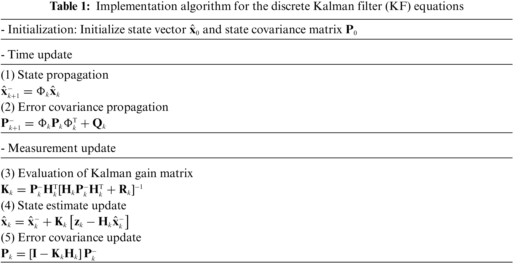
The discrete Kalman filter equations are summarized in Table 1.

On the other hand, consider a dynamical system described by a linear vector differential equation. The process model and measurement model are represented as

Process model: x˙=Fx+Gu(3)

Measurement model: z=Hx+v(4)

where the vectors u(t) and v(t) are white noise sequences with zero means and are mutually independent:

E[u(t)uT(τ)]=Qδ(t−τ);E[v(t)vT(τ)]=Rδ(t−τ);E[u(t)vT(τ)]=0(5)

where δ(t−τ) is the Dirac delta function, E[⋅] represents expectation, and superscript “T” denotes matrix transpose.

Discretisation of the continuous time system given by Eq. (3) into discrete-time equivalent form leads to

x(tk+1)=Φ(tk+1,tk)x(tk)+∫tktk+1Φ(tk+1,τ)G(τ)u(τ)dτ(6)

Using the abbreviated notation as in Eq. (1), the state transition matrix, using the Taylor’s series expansion, can be represented as

Φk=eFΔt=I+FΔt+F2Δt22!+F3Δt33!+⋯(7)

The noise input in the process model of Eq. (6) is given by

wk=∫tktk+1Φ(tk+1,τ)G(τ)u(τ)dτ(8)

where tk≡kΔt and tk+1≡(k+1)Δt. Calculation of process noise covariance leads to

Qk=E[wkwiT]=∫tktk+1Φ(tk+1,η)GQGTΦT(tk+1,η)dη(9)

The first-order approximation is obtained by setting Φk≈I

Qk≈GQGTΔt(10)

2.2 The Extended Kalman Filter

Consider a dynamical system described by a nonlinear vector difference equation. Assuming the process is to be estimated and the associated measurement relationship may be written in the form:

xk+1=f(xk,k)+wk(11)

zk=h(xk,k)+vk(12)

where xk∈ℜn, is the state vector, wk∈ℜn, is the process noise vector, zk∈ℜm, is the measurement vector, and vk∈ℜm is the measurement noise vector. The vectors wk and vk are zero mean Gaussian white sequences having zero cross-correlation with each other:

E[wkwiT]=Qkδik;E[vkviT]=Rkδik;E[wkviT]=0

where Qk is the process noise covariance matrix, and Rk is the measurement noise covariance matrix. The symbol δik stands for the Kronecker delta function:

δik={1,i=k0,i≠k

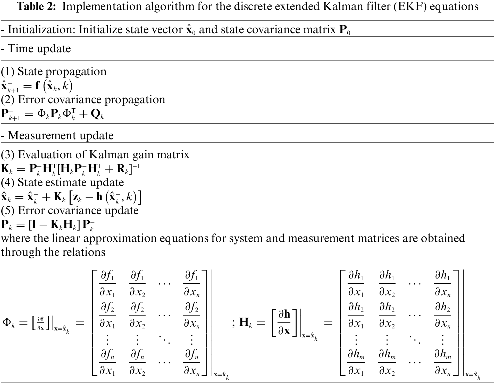
The discrete extended Kalman filter equations are summarized in Table 2.

3  System Models Discussed in This Work

The employment of proper system models enables us to analyze the behavior of the process to some extent effectively. Dynamic systems are also driven by disturbances that can neither be controlled nor modeled deterministically. The KF and EKF can be extremely sensitive to this effect during periods of relatively high state uncertainty, such as initialization and start-up. The problems that result from wrong initial estimates of x and P have been addressed and are not covered in this work. One type of divergence may arise because of inaccurate modeling of the process being estimated. Some critical issues relating to the modeling and convergence of the implementation of the Kalman filter family are of importance. Although the best cure for non-convergence caused by unmodeled states is to correct the model, this is not always easy. Additional “fictitious” process noise added to the system model assumed by the Kalman filter is an ad hoc fix. This remedy can be considering “lying” to the Kalman filter model. In addition, there are some issues with linear and nonlinear measurements of estimation performance. Parameter identification by state vector augmentation is also covered.

This article selects five models for discussion: the random constant, the random walk, the scalar Gauss-Markov process, the scalar nonlinear dynamic system, and the Van der Pol oscillator (VPO) model. The selected models are adopted to highlight the critical issues with an emphasis on convergence and modeling a step-by-step verification procedure for correct realization of the algorithms.

(1) Random constant

The random constant is a non-dynamic quality with a fixed, albeit random, amplitude. The random constant is described by the differential equation

x˙=0(x=constant, namely,x has zero slope.)(13)

which can be discretized as

xk+1=xk

(2) Random walk

The random walk process results when uncorrelated signals are integrated. It derives its name from the example of a man who takes fixed-length steps in arbitrary directions. At the limit, when the number of steps is large and the individual steps are short in length, the distance travelled in a particular direction resembles the random walk process. The differential equation for the random walk process is

x˙=u,u∼N(0,q)(14)

which can be discretized as

xk+1=xk+wk,wk∼N(0,Qk)

(3) Scalar Gauss-Markov process

A Gauss-Markov process is a stochastic process that satisfies the requirements for both Gaussian and Markov processes. The scalar Gauss-Markov process has the form:

x˙=−βx+u(15)

(4) Scalar nonlinear dynamic system

The scalar nonlinear dynamic system used in this example is given by

x˙=−(x+1)(x+3)=−(x2+4x+3)(16)

(5) Van der Pol oscillator

The Van der Pol oscillator is a non-conservative oscillator with non-linear damping. It evolves in time according to the second-order differential equation:

x¨−μ(1−x2)x˙+x=0(17)

where x is the position coordinate, which is a function of the time t, and μ is a scalar parameter indicating the nonlinearity and the strength of the damping and can be written in the two-dimensional form:

x˙1=x2(18a)

x˙2=μ(1−x12)x2−x1(18b)

4  Illustrative Examples

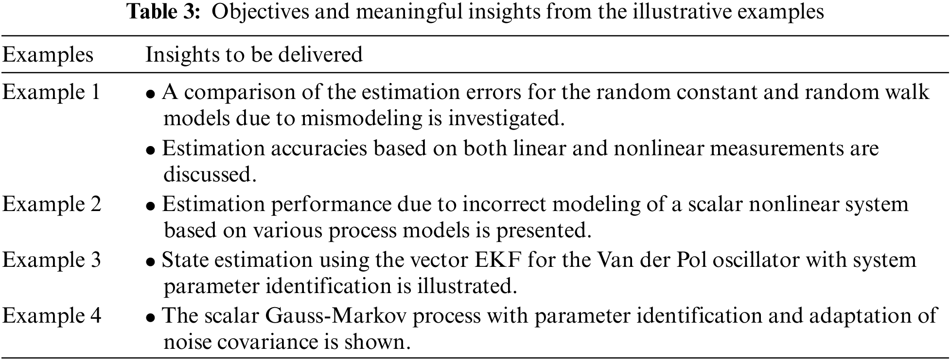
Appropriate modeling for the dynamic system is critical to its accuracy improvement and convergence assurance. Several vital issues concerning state estimation using the KF and EKF approaches will be addressed in this section. Four supporting examples are provided for illustration. Table 3 summarizes the objectives and meaningful insights from the examples.

4.1 Example 1: Random Constant vs. Random Walk

In the first example, state estimation processing for a random constant and a random walk will be discussed under various situations.

4.1.1 Estimation of a Random Constant

Firstly, consider a system dynamic that is actually a random constant but is inaccurately modeled as a random walk, where the linear measurement z=x+v is involved, as shown in Table 4. Fig. 1 presents the estimation result for the random constant (x˙=0, x=6.6 in this work) using the KF with various noise strengths (q’s) in the process model, which is a random walk model. Three q values (0, 0.001, and 0.01, respectively) are utilized. It can be seen that an increase of q decreases the estimation accuracy. In this case, the random constant model is appropriate to capture the system dynamics well. However, an increase in noise strength will decrease the estimation accuracy caused by the model mismatch. This phenomenon can be the overfitting of the system model when additional noise is introduced.

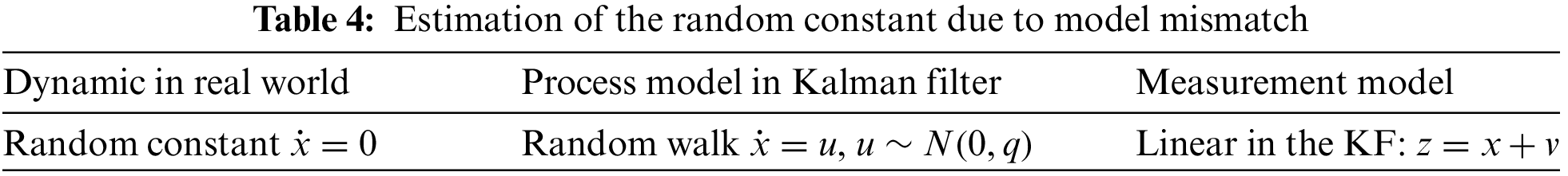
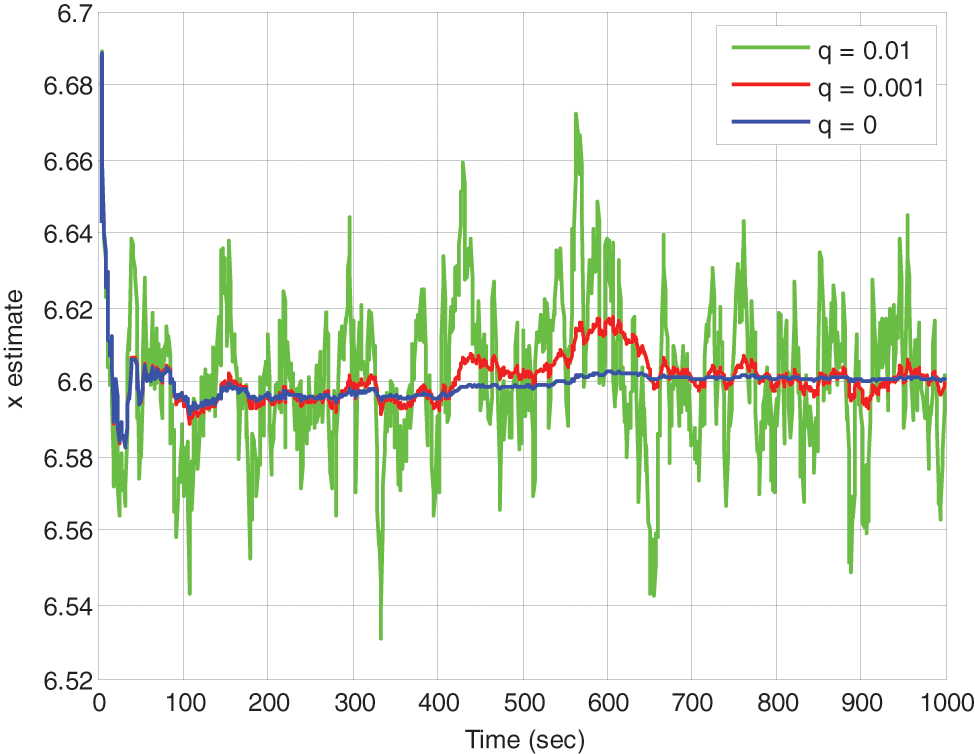
Figure 1: Estimation of the random constant using the KF with various noise strengths in the process model

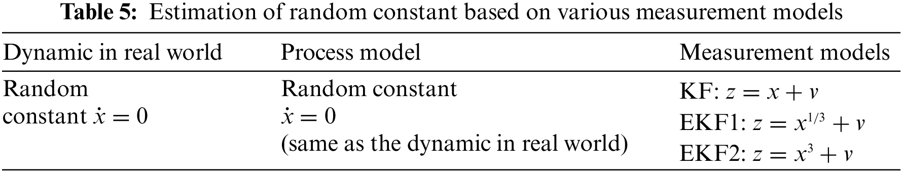
In the following cases, the KF using a linear measurement model vs. the EKF using two types of nonlinear measurement models are investigated. First, the state estimation for a random constant with the following measurement models is involved:

1.    The linear measurement z=x+v, referred to as the KF approach.

2.    Nonlinear measurement z=x1/3+v, referred to as the EKF1 approach.

3.    Nonlinear measurement z=x3+v, referred to as the EKF2 approach.

Which is summarized in Table 5.

For the EKF1 approach, the Jacobian related to the measurement is given by

H=∂h∂x=13x−2/3(19)

and for the EKF2 approach, it is given by

H=∂h∂x=3x2(20)

for the two types of nonlinear measurement models. The process noise is set as q=0 for all cases, and the same measurement noise strength has been applied for all three types of measurement models. Fig. 2 shows the estimation results of a random constant using the KF compared to the EKF utilizing the other two types of nonlinear measurements. The subplot on the right provides a closer look at their behaviors near the truth value. For EKF1 involving z=x1/3+v, the noise is relatively more substantial as compared to the state x in magnitude, leading to worse precision in state estimation; on the contrary, for EKF2 involving z=x3+v, the noise is relatively weaker as compared to the magnitude of x, leading to better/improved results.

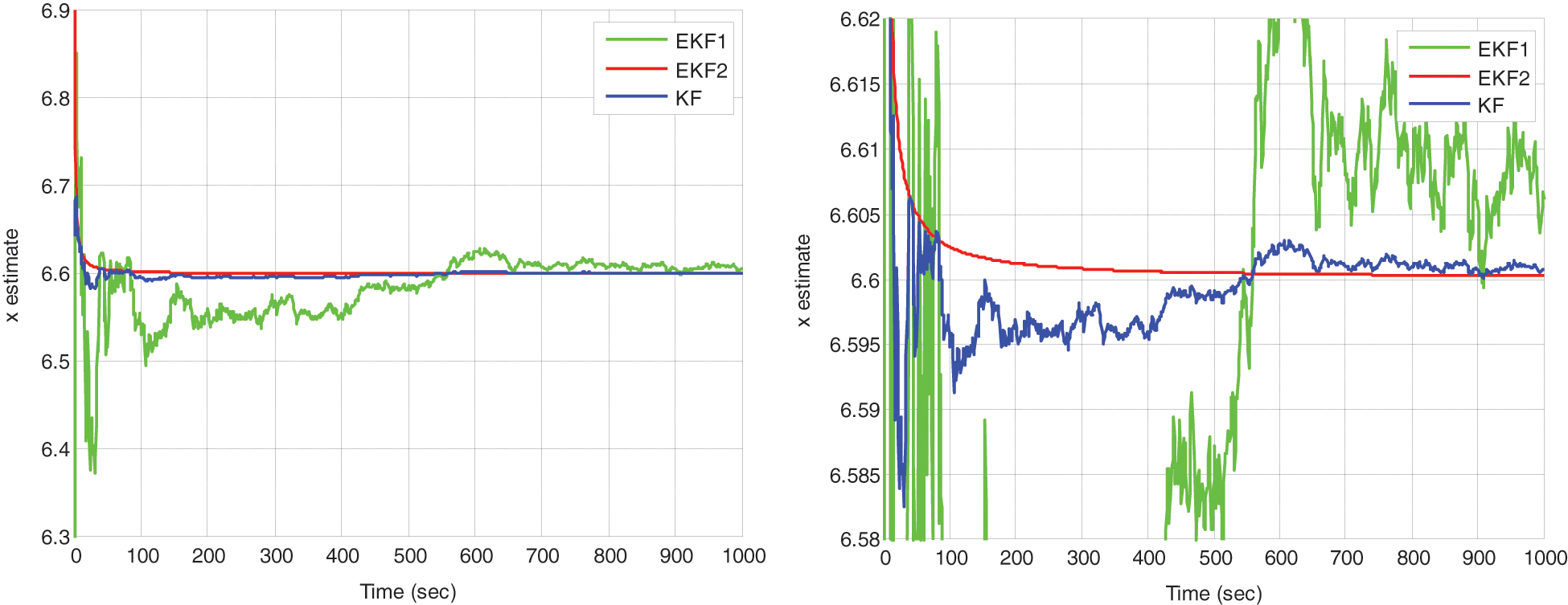
Figure 2: Estimation of the random constant using the KF and EKF utilizing two types of nonlinear measurements. The plot on the right provides a closer look at their behaviors near the truth value

4.1.2 Estimation of a Random Walk

The following demonstration considers a process that is actually a random walk process but is incorrectly modeled as a random constant, namely,

- Correct Kalman filter model: x˙=u, u∼N(0,q);

- Incorrect Kalman filter model: x=0.

This process was first processed using an incorrect model (i.e., q=0), and then using the correct model (i.e., q>0). The estimates by the filter with a correctly modeled process follow the random walk quite well. On the other hand, an incorrect process model leads to degraded results. It occurs simply because the designer “told” the Kalman filter that the process behaved differently, whereas it behaves another way. In this case, the filter is told that the process is a random constant with zero slopes. Still, the process has a nonzero slope, and the filter tries to fit the wrong curve to the measurement data. As a result, the filter with an incorrectly modeled process does very poorly due to the filter’s gain becoming less and less with each subsequent step. The Kalman gain and the covariance matrix P are correct if the models used in computing them are correct. However, the P matrix can be erroneous and of little use in detecting non-convergence in the case of mismodeling. P can even converge to zero while the state estimation error is actually diverging. Fig. 3 shows estimates of the state and the corresponding errors due to unmodeled system driving noise.

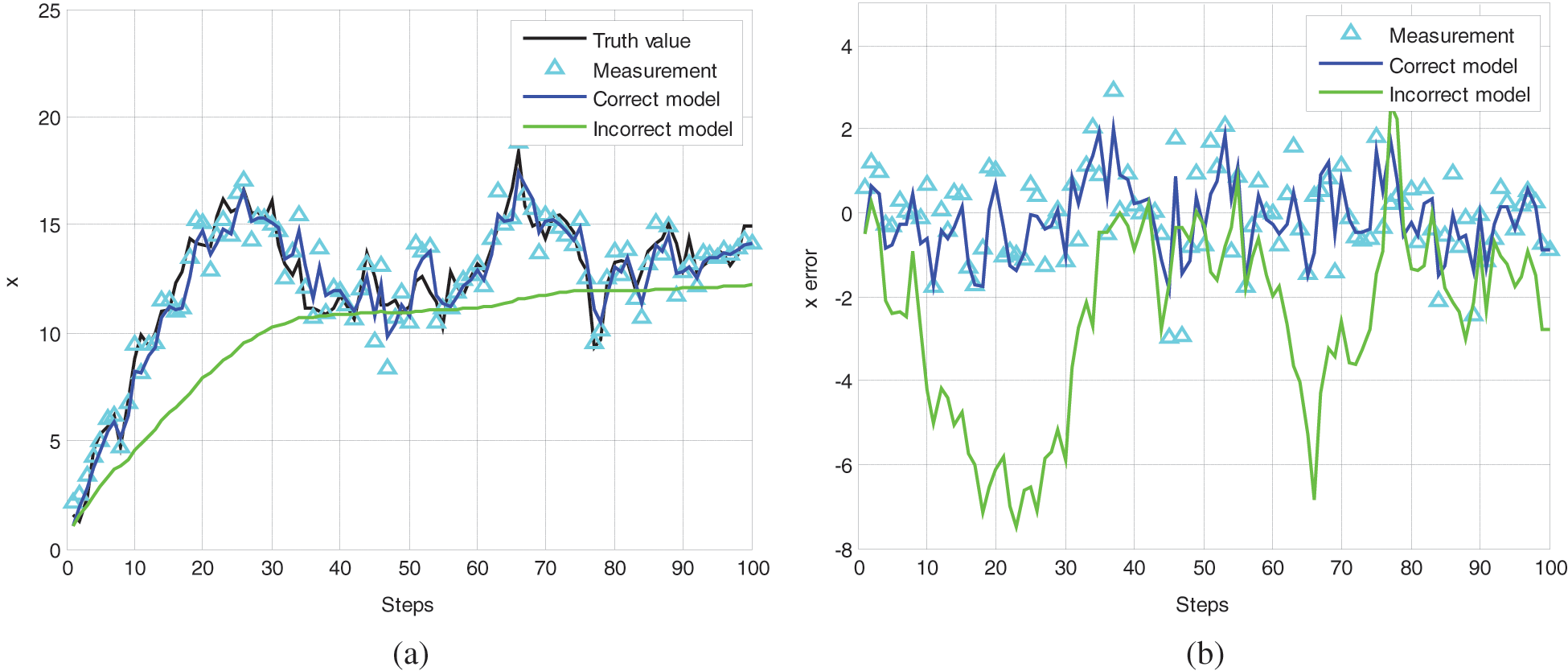
Figure 3: (a) The states and (b) the corresponding errors due to unmodeled system driving noise

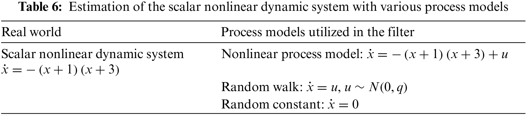
4.2 Example 2: Scalar Nonlinear Dynamic System

In the second example, consider the scalar nonlinear dynamic system

x˙=−(x+1)(x+3)=−(x2+4x+3),x(0)=−2

where the actual solution is given by x(t)=−3+2(1+e−2t)−1.

The process model will be ideally modeled as its actual nonlinear dynamic and then incorrectly modeled as a linear model, including the random walk and the random constant:

1.    Nonlinear process model: x˙=−(x+1)(x+3)+u, u∼N(0,q).

2.    Random walk model: x˙=u, u∼N(0,q).

3.    Random constant model: x˙=0.

Summarized in Table 6. The estimation performance with linear measurement (z=x+v) using the process models mentioned above will be evaluated.

State estimation results for this nonlinear dynamic system with the process model using the (ideal) nonlinear model (q≈0, meaning that the model is perfectly described except for the numerical error due to discretization, which can be cured by adding a small amount of noise) in comparison with the linear process model of random walk (q=0.01). The Jacobian related to the nonlinear dynamic process model is given by

F=∂f∂x=−2x−4(21)

Φk=eFΔt≈1+FΔt=1+(−2x−4)Δt(22)

Fig. 4 presents the estimation errors of this scalar nonlinear dynamic system using the KF with q=0.01 compared to the EKF with q=0. The truth model in this example is nonlinear but is incorrectly modeled in the process model of KF. As a result, non-convergence appears due to mismodeling. However, “lying” to the filter by adding fictitious process noise to the KF model can appropriately cure this problem. Fig. 5 provides the estimation performance using the KF and EKF. In Fig. 5, the estimation errors based on the process models using the linear ones (with q=0, 0.0001, and 0.01, respectively) and the (ideal) nonlinear model (with q=0, 0.001, and 0.01, respectively) are presented. When the additional fictitious q introduced is not sufficient to compensate for the system mismodeling, non-convergence will occur, as shown in the subplot (a) of Fig. 5. On the other hand, the case that q is more than necessary (and thus presents the phenomenon of overfitting) will lead to noisy results, as shown in the subplot (b) of Fig. 5.

Figure 4: Estimation for the nonlinear dynamic system using KF with q=0.01 and EKF with q=0

Figure 5: Estimation errors based on the (a) KF and (b) EKF with various q values

4.3 Example 3: The Van der Pol Oscillator with Parameter Identification

The nonlinear dynamic system of the Van der Pol oscillator is considered in the third example. It is a non-conservative oscillator with non-linear damping, evolving in time according to a second-order differential equation, and can be written in the two-dimensional form:

x˙1=x2

x˙2=μ(1−x12)x2−x1

where x1 is the position coordinate, a function of the time t, and μ is a scalar parameter, indicating the strength of the damping. The analytical solution of the VPO is, in general, not available or difficult to obtain. In this work, the fourth-order Runge-Kutta integrator with a sampling interval of Δt=0.001 s and x0=[0−0.5]T is used to numerically calculate the states, which is a perfect approximation of the true states. Fig. 6 provides the simulation results for the x1, x2, and the phase portraits of the VPO model. The fourth-order Runge-Kutta integrator with a sampling interval of Δt=0.001 s (in blue) and the Euler integrator with a sampling interval of Δt=0.1 s (in green), respectively, are utilized.

Figure 6: Simulation for the Van der Pol oscillator (VPO): (a) x1; (b) x2 and (c) the phase portrait

Even though a continuous-time model can precisely describe the system, the discretization of the continuous-time model may encounter non-convergence issues. It can be seen that the sampling interval for the discrete-time model derived from the continuous-time model remarkably influences the accuracy, especially for a system with relatively high nonlinearity, like this example. The error caused by numerical approximation directly reflects the estimation accuracy, which can be seen by comparing the two sets of curves. When the discrete-time version of the filter is employed, applying appropriate fictitious noise by adding Qk to cure the non-convergence is helpful.

∂f∂x=[∂f1∂x1∂f1∂x2∂f2∂x1∂f2∂x2]=[01−2μx1x2−1μ(1−x12)](23)

If the estimation is performed using the ideal nonlinear process model, namely,

x˙1=x2

x˙2=μ(1−x12)x2−x1+u

In the case that the nonlinearity parameter is unknown and is to be identified, the state variables for this problem are designated as

x1=x,x2=x˙,x3=μ(24)

we then have x=[x1x2x3]T=[xx˙μ]T. A parameter problem is then converted to a nonlinear state estimation problem. The equation of motion involving three states for the plant then becomes

ddt[x1(t)x2(t)x3(t)]=[x2x3(1−x12)x2−x10]+[010]u(t)(25)

With the process model mentioned above, the corresponding Jacobian matrix is given by

∂f∂x=[∂f1∂x1∂f1∂x2∂f1∂x3∂f2∂x1∂f2∂x2∂f2∂x3∂f3∂x1∂f3∂x2∂f3∂x3]=[010−2x1x2x3−1x3(1−x12)(1−x12)x2000](26)

The observation equation is assumed to be available in either of the linear forms:

1.    z(t)=x1(t)+v1(t), v1(t)∼N(0,r1);

2.    z=[1001][x1x2]+[v1v2], vi∼N(0,ri), i=1,2

The estimation accuracy of the states highly relies on the measurement quality and is essential to the identification performance of the unknown parameter. Figs. 7 and 8 show the state estimates and the corresponding errors of x1 and x2, respectively, for the VPO model, where the results are compared based on one and two measurements. In addition, the triangles in Fig. 7 denote the measurements. Identification of the nonlinearity parameter μ is shown in Fig. 9. The performance based on two measurements outperforms that of one.

Figure 7: Estimation of (a) the state x1 and (b) the corresponding errors based on one and two measurements, respectively

Figure 8: Estimation of (a) the state x2 and (b) the corresponding errors based on one and two measurements, respectively

Figure 9: Identification results for the nonlinearity parameter μ are based on one and two measurements, respectively

4.4 Example 4: Scalar Gauss-Markov Process Involving Adaptation of Noise Covariance

The scalar Gauss-Markov process, as described by the differential equation

x˙=−βx+u,u∼N(0,q)

can be represented by the transfer function

xu=1s+β

The continuous-time equation can be discretized as

xk+1=e−βΔtxk+uk,uk∼N(0,Qk)(27)

where the covariance

Qk=e[xk2]=q2β(1−e−2βΔt)(28)

Initially linear, the process model becomes nonlinear when performing the state estimation for the scalar Gauss-Markov process with an unknown parameter β. Notice that in this case, there are now two state variables involved:

x=[x1x2]T=[xβ]T(29)

Since the state dynamic for this problem is given by

x˙1=−x2x1+u,x˙2=0,u∼N(0,q)(30)

the process model can be represented as

[x˙1x˙2]=[−x2x10]+[10]u(31)

The problem now becomes a state estimation problem using the vector EKF. Since the two states are closely coupled, the state’s estimation accuracy will influence the parameter identification performance. In this case, the noise strength is related to the parameter to be identified, so better modeling involving Qk adaptation results in improved estimation accuracy.

In this example, the linear measurement is again assumed to be available in continuous form

z(t)=x1(t)+v(t),v(t)∼N(0,r)

The process noise covariance matrix in the discrete-time model can be written as

Qk=[q2x2(1−e−2x2Δt)000](32)

Fig. 10 shows the results of identifying parameter β for the scalar Gauss-Markov process. In the numerical experiment, three values of β (0.5, 1.0, and 1.5, respectively) were tested, and perfect results were obtained for all the cases. The EKF can identify the parameter β very well if the adaptation of noise statistics is included and updated in the estimation process. On the other hand, if the noise adaptation procedure is not included, the estimation error, as indicated by the curve in green, clearly shows performance degradation.

Figure 10: Identification of parameter β for the scalar Gauss-Markov process

5  Conclusion

This paper presents an introductory critical exposition of the state estimation based on the Kalman filter and the extended Kalman filter algorithms, both qualitatively and quantitatively. The article conveys an excellent conceptual explanation of the topic with illustrative examples so that the readers can grasp the proper interpretation and realization of the KF and EKF algorithms before conducting more complex systems using advanced filtering methodologies. The material covered in this work delineates the theory behind linear and nonlinear estimation with supporting examples for the discussion of important issues with emphasis on convergence and modeling. The article can help better interpret and apply the topic and make a proper connection to probability, stochastic processes, and system theory.

System stability and convergence are the basic requirements for the system design, while the performance of filtering optimality requires subtle examination for verification. One non-convergence problem may arise due to inaccurate modeling of the estimated process. Although the best cure for non-convergence caused by unmodeled states is to correct the model, this is not always easy. Some critical issues related to the modeling and convergence of implementing the Kalman filter and extended Kalman filters are emphasized with supporting examples. Adding fictitious process noise to the system model assumed by the Kalman filter for convergence assurance is discussed. Details of dynamic modeling have been discussed, accompanied by selected examples for a clear illustration. Some issues related to linear and nonlinear measurements are involved. Parameter identification by state vector augmentation is also demonstrated. A detailed description with examples of problems is offered to gives readers a better understanding of this topic. This work provides a step-by-step illustration, explanation and verification. The lesson learned in this paper enables the readers to appropriately interpret the theory and algorithms, and precisely implement the computer codes that nicely match the estimation algorithms related to the mathematical equations. This is especially helpful for those readers with less experience or background in optimal estimation theory, as it provides a solid foundation for further study on the theory and applications of the topic.

This article elaborates on several important issues and highlights the checkpoints to ensure the algorithms are appropriately implemented. Future work may be extended to the design of position tracking and control for robots, the navigation processing for inertial navigation and the Global Positioning System, etc. Once the KF and EKF algorithms can be accurately and precisely implemented, further advanced designs dealing with highly nonlinear and sophisticated systems using advanced estimators such as the UKF and CKF, as well as robust filters become possible and reliable.

Acknowledgement: Thanks to Dr. Ta-Shun Cho of Asia University, Taiwan for his assistance in the course of this research.

Funding Statement: This work has been partially supported by the Ministry of Science and Technology, Taiwan (Grant Number MOST 110-2221-E-019-042).

Author Contributions: The author confirms contribution to the paper as follows: study conception and design: D.-J. Jwo; data collection: D.-J. Jwo; analysis and interpretation of results: D.-J. Jwo; draft manuscript preparation: D.-J. Jwo. The author reviewed the results and approved the final version of the manuscript.

Availability of Data and Materials: The data used in this paper can be requested from the author upon request.

Conflicts of Interest: The author declares that they have no conflicts of interest to report regarding the present study.

References

1. R. E. Kalman, “A new approach to linear filtering and prediction problems,” Transactions of the ASME–Journal of Basic Engineering, vol. 82, no. 1, pp. 35–45, 1960. [Google Scholar]

2. R. G. Brown and P. Y. C. Hwang, Introduction to Random Signals and Applied Kalman Filtering. New York, NY, USA: John Wiley & Sons, Inc., pp. 214–225, 1997. [Google Scholar]

3. M. S. Grewal and A. P. Andrews, Kalman Filtering, Theory and Practice Using MATLAB, 2nd ed., New York, NY, USA: John Wiley & Sons, Inc., pp. 114–201, 2001. [Google Scholar]

4. A. Gelb, Applied Optimal Estimation. Cambridge, MA, USA: M.I.T. Press, pp. 102–228, 1974. [Google Scholar]

5. F. L. Lewis, L. Xie and D. Popa, Optimal and Robust Estimation, with an Introduction to Stochastic Control Theory, 2nd ed., Boca Raton, FL, USA: CRC Press, pp. 3–312, 2008. [Google Scholar]

6. S. P. Maybeck, Stochastic Models, Estimation, and Control, vol. 2. New York, NY, USA: Academic Press, pp. 29–67, 1982. [Google Scholar]

7. Y. Bar-Shalom, X. R. Li and T. Kirubarajan, Estimation with Applications to Tracking and Navigation. New York, NY, USA: John Wiley & Sons, Inc., pp. 491–535, 2001. [Google Scholar]

8. J. A. Farrell and M. Barth, The Global Positioning System & Inertial Navigation. New York, NY, USA: McCraw-Hill, pp. 141–186, 1999. [Google Scholar]

9. S. Karthik, R. S. Bhadoria, J. G. Lee, A. K. Sivaraman, S. Samanta et al., “Prognostic kalman filter based Bayesian learning model for data accuracy prediction,” Computers, Materials & Continua, vol. 72, no. 1, pp. 243–259, 2022. [Google Scholar]

10. Mustaqeem and S. Kwon, “A CNN-assisted enhanced audio signal processing for speech emotion recognition,” Sensors, vol. 20, no. 1, pp. 183, 2020. [Google Scholar]

11. Mustaqeem, M. Ishaq S. and Kwon, “Short-term energy forecasting framework using an ensemble deep learning approach,” IEEE Access, vol. 9, no. 1, pp. 94262–94271, 2021. [Google Scholar]

12. B. Maji, M. Swain and Mustaqeem, “Advanced fusion-based speech emotion recognition system using a dual-attention mechanism with Conv-Caps and Bi-GRU features,” Electronics, vol. 11, no. 9, pp. 1328, 2022. [Google Scholar]

13. S. Sund, L. H. Sendstad and J. J. J. Thijssen, “Kalman filter approach to real options with active learning,” Computational Management Science, vol. 19, no. 3, pp. 457–490, 2022. [Google Scholar] [PubMed]

14. G. Welch and G. Bishop, “An introduction to the kalman filter,” Technical Report TR 95-041, University of North Carolina, Department of Computer Science, Chapel Hill, NC, USA, 2006. [Online]. Available: https://www.cs.unc.edu/~welch/media/pdf/kalman_intro.pdf [Google Scholar]

15. C. M. Kwan and F. L. Lewis, “A note on kalman filtering,” IEEE Transactions on Education, vol. 42, no. 3, pp. 225–228, 1999. [Google Scholar]

16. K. Wang, “Textbook design of kalman filter for undergraduates,” in Proc. of the Int. Conf. on Information, Business and Education Technology (ICIBET 2013), Beijing, China, pp. 891–894, 2013. [Google Scholar]

17. Y. Kim and H. Bang, “Introduction to Kalman filter and its applications,” in Introduction and Implementations of the Kalman Filter. London, UK: IntechOpen, pp. 1–16, 2018. [Online]. Available: https://cdn.intechopen.com/pdfs/63164.pdf [Google Scholar]

18. M. B. Rhudy, R. A. Salguero and K. Holappa, “A kalman filtering tutorial for undergraduate students,” International Journal of Computer Science & Engineering Survey (IJCSES), vol. 8, no. 1, pp. 1–18, 2017. [Google Scholar]

19. A. Love, M. Aburdene and R. W. Zarrouk, “Teaching kalman filters to undergraduate students,” in Proc. of the 2001 American Society for Engineering Education Annual Conf. & Exposition, Albuquerque, NM, USA, pp. 6.950.1–6.950.19, 2001. [Google Scholar]

20. A. M. S. Mahdy, “Numerical studies for solving fractional integro-differential equations,” Journal of Ocean Engineering and Science, vol. 3, no. 2, pp. 127–132, 2018. [Google Scholar]

21. A. M. S. Mahdy, Y. A. E. Amer, M. S. Mohamed and E. Sobhy, “General fractional financial models of awareness with Caputo–Fabrizio derivative,” Advances in Mechanical Engineering, vol. 12, no. 11, pp. 1–9, 2020. [Google Scholar]

22. A. M. S. Mahdy, “Numerical solutions for solving model time-fractional Fokker-Planck equation,” Numerical Methods for Partial Differential Equations, vol. 37, no. 2, pp. 1120–1135, 2021. [Google Scholar]

23. M. Chen, “The SLAM algorithm for multiple robots based on parameter estimation,” Intelligent Automation & Soft Computing, vol. 24, no. 3, pp. 593–602, 2018. [Google Scholar]

24. A. A. Afonin, D. A. Mikhaylin, A. S. Sulakov and A. P. Moskalev, “The adaptive kalman filter in aircraft control and navigation systems,” in Proc. of the 2nd Int. Conf. on Control Systems, Mathematical Modeling, Automation and Energy Efficiency (SUMMA), Lipetsk, Russia, pp. 121–124, 2020. [Google Scholar]

25. Y. Huang, M. Bai, Y. Li, Y. Zhang and J. Chambers, “An improved variational adaptive kalman filter for cooperative localization,” IEEE Sensors Journal, vol. 21, no. 9, pp. 10775–10786, 2021. [Google Scholar]

26. N. Arulmozhi and T. Aruldoss Albert Victorie, “Kalman filter and H∞ filter based linear quadratic regulator for furuta pendulum,” Computer Systems Science and Engineering, vol. 43, no. 2, pp. 605–623, 2022. [Google Scholar]