Design Optimization of Permanent Magnet Eddy Current Coupler Based on an Intelligence Algorithm

1  Introduction

The permanent magnet eddy current coupler (PMEC) is a kind of equipment that uses the force between magnetic fields to transfer torque and whose outstanding feature is no mechanical connection. This noncontact structure has the benefits of vibration isolation, alignment error tolerance, and overload protection while lowering friction and equipment loss [1]. When PMEC works, the induced eddy current in the conductor provides torque for the load. However, it also causes heat to be produced and energy to be lost, which lowers the effectiveness of energy transfer. Multi-objective optimization is an excellent method to balance the transmission performance and eddy current loss of PMEC. A trustworthy model is required to predict the performance of PMEC throughout the optimization process [2].

There are three common modeling methods for PMEC. The first is to use the method of separating variables to solve partial differential equations based on Maxwell equations and boundary conditions [3–8]. The second is to build an equivalent magnetic circuit (EMC) based on the similarity between the magnetic circuit and the circuit and then solve it according to Kirchhoff’s law and Ohm’s law of the magnetic circuit [9–13]. The influence of eddy currents should be considered in the modeling process of PMEC. However, EMC is a method that does not consider eddy current, and the existing EMC models cannot directly calculate eddy current effects [10]. Although the calculations for these two methods are simple, the modeling process necessitates several assumptions and simplifications, as well as the application of numerous empirical components, which causes the calculation results from the model to diverge from the actual scenario. Additionally, these models often predict the performance of PMEC with reasonable accuracy at low relative slips, but as relative slip increases, the accuracy of the models rapidly decreases [14]. The third method is the numerical method, such as the finite element method (FEM), which enables the analysis of electromagnetic field problems from the classical analytical method to the numerical analysis method of discrete systems so that high-precision discrete solutions can be obtained [15–17]. The FEM can produce accurate results, but because of its extensive calculation and time requirement, it is often used for verification. Neural networks are frequently used for numerical prediction in complex situations. There are, however, few studies that use neural networks to predict PMEC performance. In light of this, this paper suggests a Levenberg-Marquardt back propagation (LMBP) neural network-based modeling approach for PMEC.

Numerous intelligent optimization algorithms have been used to address the multi-objective optimization of electromagnetic equipment. References [2] and [18] used the genetic algorithm (GA) to carry out multi-objective optimization for dual-sided radial PMEC and radial flux permanent magnet motors. Reference [19] has optimized and designed the inner-mounted permanent magnet synchronous motor (IPMSM) by correlating the particle swarm optimization algorithm (PSO) with the FEM. References [20] and [21] used an improved PSO to optimize the energy consumption of tram operations. However, these methods use weighted methods to integrate multiple objective functions into one. The solutions obtained in these ways are closely related to the defined weights and have high subjectivity. To address the issues raised above, references [22–24] adopted multi-objective particle swarm optimization (MOPSO) based on Pareto optimal sequencing. Although they proposed various MOPSO improvement strategies, finding a globally optimal solution is still challenging since diversity and convergence are tricky to balance.

This paper aims to investigate the multi-objective optimization design method of PMEC structural parameters to simultaneously improve transmission performance, suppress eddy current loss, and lower material cost. A PMEC modeling method based on the LMBP neural network is proposed. The nonlinear regression model of PMEC is established in the whole space to compensate for the theoretical model’s low accuracy, which combines the ANSYS simulation data with the LMBP neural network. Then, to balance the convergence and diversity of MOPSO, the novel competitive mechanism-based multi-objective particle swarm optimization algorithm (NCMOPSO) is proposed and applied to the parameter optimization of PMEC. This method can calculate all feasible nondominated optimal solutions, avoiding the subjectivity and complexity of the objective function mechanism caused by the weighting method. Chaotic search and mutation strategies are used to enhance the diversity of the population, which improves the problem of a too-fast rate of convergence of the algorithm. Finally, the LMBP model’s accuracy and the optimization algorithm’s effectiveness are verified by MATLAB and finite element simulation, respectively.

2  LMBP Neural Network Model of PMEC

2.1 Structure and Working Principle of PMEC

The mechanical structure of PMEC with a single-group disk structure is shown in Fig. 1. The conductor rotor and PM rotor can rotate independently. When PMEC works, the conductor rotor is driven by a motor to rotate, cutting off the magnetic induction lines generated by PM and forming eddy currents. Near the conductor disk, eddy current, in turn, generates an induced magnetic field. According to Lenz’s law, the eddy current magnetic field should prevent the relative movement between the PM rotor and the conductor rotor by preventing the change of magnetic flux caused by the eddy current. Under the interaction between the eddy current magnetic field and the permanent magnetic field, the PM rotor lags behind the conductor rotor, which realizes the torque transfer from the motor to the load.

Figure 1: Mechanical structure of PMEC

2.2 Levenberg-Marquardt Back Propagation Neural Network

The neural network can approximate arbitrary complex nonlinear systems. The BP neural network based on the gradient descent (GD) method is the most successful and widely used neural network learning algorithm [25]. However, its slow convergence speed makes it easy to fall into local extreme values. The LMBP neural network uses the Levenberg-Marquardt (LM) algorithm instead of the GD method to solve the optimization problem. It combines the GD and Gauss-Newton methods and benefits from their global characteristics and efficient convergence. Moreover, it has advantages in solving various nonlinear problems [26]. The formula for the modified weight is as follows:

x(k+1)=x(k)−JT(x)E(x)JT(x)J(x)+uI(1)

where JT(x) is the Jacobian matrix, E(x) is the network error vector, I is the identity matrix, and u is the damping term. The objective function is the square error function, as shown in Eq. (2).

E(x)=12∑i=1Nei2(x)(2)

where ei(x) is the error between the ith predicted value and the actual value.

If u=0, the LM algorithm becomes a Gauss-Newton method using an approximate Hessian matrix. If u is large, it becomes a small step GD. The purpose of the LM algorithm is to convert to the Newton method as quickly as possible. Since it converges faster and has higher accuracy near the minimum error point. If an iteration succeeds and the error performance function decreases, then the value of u will be reduced. If the iteration fails, the value of u will be increased. In this way, error performance can be minimized with iteration.

2.3 Modeling of PMEC Based on LMBP Neural Network

2.3.1 Determination of Input and Output of the Model

PMEC is a complex multivariable coupling input and output system. The main structural parameters affecting the PMEC output performance are the thickness of the copper disk and the thickness, length, and width of the PM. Therefore, these four variables are selected as the model’s input variables. The model’s output variables are the PMEC’s output torque and eddy current loss. The impact of input variables on output variables is analyzed as follows:

•   Copper disk thickness: During operation, the copper disk generates an eddy current and provides a flow circuit for the eddy current. Its thickness will directly affect the resistance in the eddy current circuit and then affect the eddy current loss and output torque.

•   The volume of PM: Increasing PM volume will inevitably result in rising magnetic flux and magnetic potential. However, at the same time, the magnetic resistance and leakage in the magnetic circuit will also increase, consuming the increased magnetic potential and decreasing the remaining magnetic flux of PM. The growth rate is reducing while the output torque and eddy current loss are rising.

The LMBP neural network model structure of PMEC is shown in Fig. 2.

Figure 2: Structure of PMEC neural network model

2.3.2 Sample Point Selection and Pretreatment

The accuracy of sample data determines the reliability of neural network modeling. Establish a PMEC model using ANSYS Maxwell software. Conduct finite element simulation to obtain relevant data on its torque characteristics and eddy current loss as the LMBP neural network training samples.

This paper takes a 30 kW PMEC as an example, and Table 1 shows the prototype parameters. According to the parameters, establish its three-dimensional finite element simulation model. Through finite element calculation, the influence of four input variables of PMEC on torque performance and eddy current loss is shown in Fig. 3.

Figure 3: Influence of input variables on output torque and eddy current loss

To ensure assembly, the influence of material strength, performance, and heat dissipation is comprehensively considered. The range of input variables is shown in Table 2.

Because the units and order of magnitude of the input parameters are inconsistent, the parameters are normalized using the following equation to remove discrepancies:

y=x−xminxmax−xmin(3)

where y represents the processed data, x represents the original sample data, xmax represents the maximum value of the sample data, and xmin represents the minimum value of the sample data.

2.3.3 Neural Network Topology and Parameter Selection

The LMBP neural network has an unknown number of hidden layers and hidden layer nodes. Therefore, it is necessary to determine a more appropriate value through experiments. Since the model parameters in this study are not complicated, the number of hidden layers is determined to be one according to the Kolmogorov theorem. The range of hidden layer node points can generally be obtained from the empirical equation:

n=xin+yout+α(4)

where n is the number of hidden nodes, xin is the number of input nodes, yout is the number of output nodes, and the range of α is 1<α<10.

The number of input layer nodes equals the number of input variables, which is 4. The output variable is the eddy current loss or output torque, so the number of output nodes should be 1. According to Eq. (4), the number of hidden layer nodes ranges from 3 to 12. Experiments on models with different hidden layer nodes yield the corresponding number of iterations and mean square error (MSE) to select the optimal setting value. The experimental results are shown in Fig. 4. The training outcomes of each model are the average after ten pieces of training to ensure the reliability of the experimental results.

Figure 4: Number of neurons in the hidden layer, number of iterations and MSE

It can be seen from Fig. 4a that the model of output torque and eddy current loss is optimal when the hidden layer nodes are 10 and 11, respectively.

3  Verification of the Established Mode

3.1 Model Training and Result Comparison

The input variables of the neural network are the thickness of the copper disk and the thickness, length, and width of the PM, while the output is the output torque or eddy current loss. Train and test based on 530 data sets obtained from finite element calculations. Among them, four hundred twenty-four data groups are randomly assigned as a sample set for training. Fifty-three data groups are used as validation data sets, and the remaining 53 are used as test sets for post-training tests.

The LMBP and standard BP neural networks are trained under the same conditions to compare the training effect. Fig. 5 shows the change in MSE in both training processes.

Figure 5: The learning curve of the neural network

It can be seen from Fig. 5 that compared to the standard BP neural network, the LMBP neural network has a faster convergence speed and higher training accuracy. Use the test set to compare the MSE of the two prediction results, and its prediction results are significantly better.

3.2 Error Analysis of the Model

Fig. 6 shows the regression analysis of output torque and eddy current loss data. Almost all sample points are near the zero-error line, indicating that the regression line fits the observed values well and that the trained model is accurate and reliable.

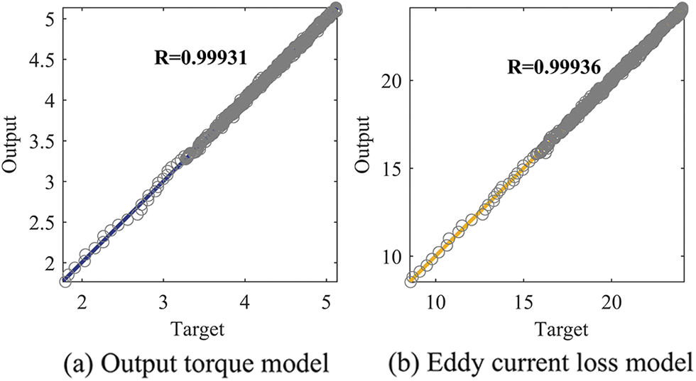
Figure 6: Regression analysis diagram of output torque and eddy current loss data

To test the training network’s generalization ability, select 70% of the samples as training samples and the balance as verification samples. Train the LMBP neural network with training samples, and test the generalization ability of the trained LMBP neural network with validation samples. The network model is run ten times under identical conditions. The projected output values are then statistically analyzed, and their MSE is calculated.

Table 3 shows the maximum, minimum, and average MSE values in the 10 test results of the LMBP neural network and the standard BP neural network. The PMEC model established using the LM algorithm to improve the BP neural network has superior prediction accuracy and generalization capacity. Furthermore, the modeling results based on standard BP neural networks fluctuate more violently. In the output torque and eddy current loss model of PMEC, the difference between the maximum and minimum MSE values of the standard BP neural network is 0.0103 and 0.4791, respectively, while the difference based on LMBP neural network modeling is only 0.0003244 and 0.0106, respectively. Therefore, the prediction output based on LMBP neural network modeling is more stable.

4  Multi-Objective Optimization Design of PMEC

4.1 Novel Competitive Mechanism-Based MOPSO

In MOPSO, the diversity of the population mainly comes from the difference between personal optimum and global optimum. Due to the global influence of the global optimum, the personal optimum may be similar to it or even have the same value, resulting in a reduction in population diversity [27]. In order to eliminate their impact on diversity, a competition mechanism is introduced to improve MOPSO.

4.1.1 Competitive Swarm Optimizer (CSO)

CSO introduces the survival competition mechanism of the fittest in biology based on PSO. In each iteration, particles are not updated with their personal and global optimums. Instead, they are randomly paired for comparison and update the loser with the winner’s information, thereby avoiding premature convergence and increasing the variety of the population.

Take the minimization problem as an example. First, initialize a population p(t) containing N particles, where N is the population size and t is the number of iterations. Randomly divide each generation’s particle population p(t) into N/2 pairs. Then select a pair of particles to compete according to their fitness values. Those particles with smaller fitness values are called winners and will enter the next generation p(t+1) directly. The losers with large fitness values must learn from the winners to update their position and velocity vectors to enter the next generation. One iteration has been completed when all particles are transferred to the next generation.

The updated formulas for the velocity vector and position vector of the loser after the competition are as follows:

Vlo,k(t+1)=R1(k,t)Vlo,k(t)+R2(k,t)(Xwi,k(t)−Xlo,k(t))+φR3(k,t)(X¯k(t)−Xlo,k(t))(5)

Xlo,k(t+1)=Xlo,k(t)+Vlo,k(t+1)(6)

where Xwi,k(t),Xlo,k(t),Vwi,k(t) and Vlo,k(t) respectively represent the position vector and velocity vector of the winner and loser in the kth round of iteration t, R1(k,t),R2(k,t) and R3(k,t) are three random vectors distributed in [0,1]n, X¯k(t) is the average position value of all contemporary particles, and φ is the control parameter to adjust the influence of X¯k(t).

4.1.2 Motivation and Framework of NCMOPSO

Although CSO can improve the diversity of PSO, there are several limitations. First, the diversity of winners in the parent generation has not improved. Because winners directly enter offspring without position updating. Chaotic search can be used to deal with the winners because chaotic dynamics have the characteristics of ergodicity, randomness, and irregularity. Second, if the parent population lacks diversity, the population will converge prematurely. Therefore, the mutation strategy can be used to avoid the population falling into a local optimum.

Algorithm 1 shows the framework of the NCMOPSO. Its major cycle mainly includes an update strategy based on the novel competition mechanism and environmental selection. They will be detailed in the following sections.

4.1.3 The Novel Competition Mechanism

The proposed competition mechanism includes pairwise competition, particle update, and mutation. In pairwise competition, the population p(t) is randomly divided into N/2 pairs. Then, compare the dominance relationship between the two particles in each pair according to the Pareto dominance relationship. If one particle can dominate the other, the dominant particle is the winner. If the two particles are nondominated by each other, select the winner according to the crowding distance ranking in the nondominated sorting genetic algorithm-II (NSGA-II) [28].

After the winner is determined, the loser’s position vector and velocity vector are updated by learning from the winner. The updated equations are Eqs. (5) and (6) in CSO. In order to improve the diversity of the winners, an update strategy was designed based on a chaotic search. It is based on the well-known logistic equation [29], which is defined as:

zn+1=μ⋅zn(1−zn)n=0,1,2⋯(7)

where zn is a variable, and μ is a control parameter. When μ=4, an utterly chaotic sequence can be iterated from any initial value z0∈[0,1].

The primary measure to update the winner is to use the ergodicity of chaotic dynamics to search for the winner and generate chaotic sequences. The process of chaotic search is defined as:

pim+1=4⋅pim(1−pim)(8)

where pi is the ith chaotic variable, m represents the number of chaotic search iterations, and pim distribution in [0,1] requires pi0∈(0,1). After each competition, the winner particle is iterated M times using Eq. (8) to generate a chaotic sequence of size M. Calculate the fitness value and crowding distance of particles in the chaotic sequence, and then select the best particle to update the original winner.

The rapid convergence of MOPSO may cause the population to gather around some particles or a specific area prematurely, thus losing diversity. Therefore, after the particles are updated, a time-varying mutation strategy is designed to mutate the particles based on the idea of [30]. The mutation formula is shown below:

xi(t+1)={xi(t)+cg(u(j)−l(j))Pmut,Pmut≥randxi(t),Pmut<rand(9)

Pmut=(1−tTmax)5Km(10)

where Pmut is the probability of mutation, Tmax is the maximum number of iterations, t is the current number of iterations, cg is the random number subject to the Gaussian distribution with a mean value of 0 and variance of 1, u(j) and l(j) are the upper bound and lower bound of the jth dimension decision variable respectively, and Km is the mutation parameter.

The detailed process of the updating strategy based on the novel competition mechanism is shown in Algorithm 2.

4.1.4 Environmental Selection Strategy

During the initial iteration, few Pareto optimal solutions will lead to poor competitiveness and convergence. However, a too-large Pareto optimal solution set in the later iteration period will lead to insufficient diversity. The angle-penalty distance (APD) proposed in the reference vector-guided evolutionary algorithm (RVEA) [31] can dynamically balance convergence and diversity in the optimization process according to the number of targets and the number of iterations. The APD between reference vectors and particles in RVEA is calculated as the following equation:

APDr∈R,pi∈P(pi,r)=(1+D(tTmax)2⟨G(pi),r⟩mins∈R,s≠r⟨s,r⟩)||G(pi)||(11)

where D is the dimension of the target space, R is the set of reference vectors, t is the number of iterations, and Tmax is the maximum number of iterations. G(pi) is the target vector of the particle pi, ⟨G(pi),r⟩ and ⟨s,r⟩ are the angles between G(pi) and r, and between s and r, respectively.

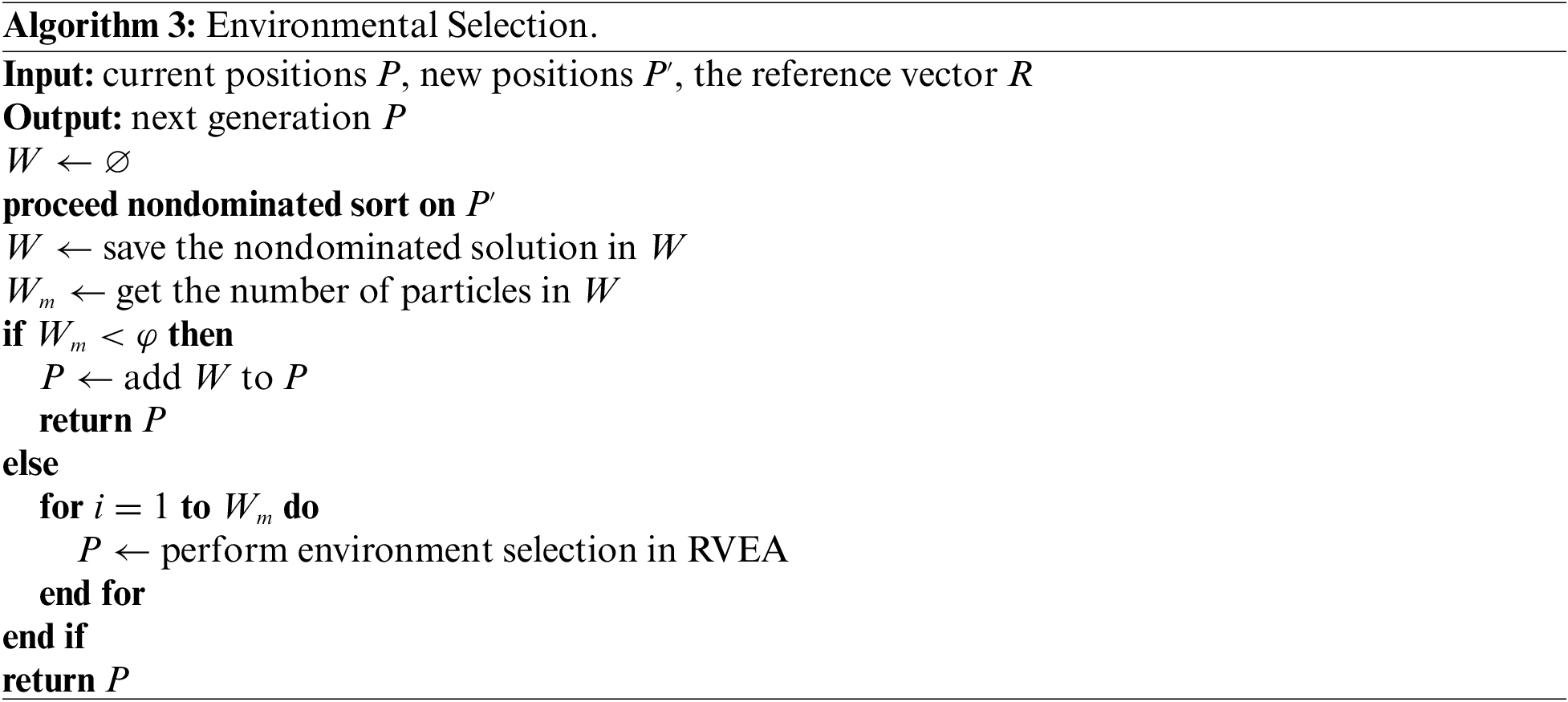
The environmental selection proposed in RVEA can be used based on constraining the size of the nondominant solution set. When the size of the nondominant solution set is smaller than γ, the nondominant solution and parent directly enter the next generation. When the size of the nondominant solution set is larger than γ, the new nondominant solution set is determined through the environmental selection of the RVEA algorithm. The study of Pareto optimal solution set size constraints in adaptive competitive multi-objective swarm algorithm based on inverse modeling [32] shows that the effect is best when γ=N/20. Algorithm 3 shows the details of the environmental selection strategy.

4.2 Multi-Objective Optimization Model of PMEC

According to the analysis of different structural parameters in Chapter 2, the thickness of the copper disk and the thickness, length, and width of the PM are selected as decision variables. The optimization goal is to increase output torque while decreasing eddy current loss and cost. The LMBP neural network fits the fitness functions of output torque and eddy current loss. The cost is also of great significance in the design of PMEC, mainly from the copper disk, PM, and back iron materials. In order to simplify the calculation, it is assumed that the price of the PM is ten times the price of the copper disk and the back iron. Then the approximate fitness function of the cost can be expressed as:

{V=voldriver+10volmagnet=πrav2W+10Nmx2x3x4pW=x1+2sb(12)

where rav is the average radius of the copper disk of PMEC, Nm is the number of permanent magnets, x1 is the width of the thickness of the copper disk, x2,x3 and x4 are the thickness, length, and width of PM, respectively, and sb is the thickness of the back iron.

There is the multi-objective optimization model of PMEC:

{minPloss=f1(X)          s.t.2≤x1≤10maxT=f2(X)                           4≤x2≤12minV=f3(X)                            10≤x3≤50                                                                      25≤x4≤75(13)

where X=(x1,x2,x3,x4), f1(X),f2(X) is the functional relationship of PMEC eddy current loss and output torque concerning decision variables established by the LMBP neural network, respectively, and f3(X) is the functional relationship between PMEC cost and decision variables. Fig. 7 shows the specific optimization process for PMEC.

Figure 7: Flow chart of the optimization process

5  Optimization Results and Analysis

In order to verify the performance of NCMOPSO, it is compared with the popular NSGA-II [28], dominance-weighted uniformity (DWU) multi-objective evolutionary algorithm [33], direction-guided evolutionary algorithm (DGEA) [34], and existing PSOs such as MOPSO with multiple search strategies (MMOPSO) [35], speed-constrained multi-objective particle swarm optimization (SMPSO) [36], multi-objective particle swarm optimization algorithm based on decomposition (MPSOD) [37], and MOPSO [38]. To be fair, the parameters used in the comparison algorithm are the original paper’s recommended values. Table 4 shows the parameters of the proposed NCMOPSO.

The proposed NCMOPSO and seven other multi-objective optimization algorithms are applied to the optimization model of PMEC, and the resulting solution is shown in Fig. 8.

Figure 8: Solution set obtained by proposed NCMOPSO and other optimization algorithms

In Fig. 8, f1 is eddy current loss, f2 is output torque, and f3 is the cost of PMEC. The particle distribution in the solution set obtained by the proposed NCMOPSO is more uniform and extensive than that of other optimization algorithms, which indicates that it solves the problem of poor diversity in MOPSO to a certain extent.

To make a more comprehensive evaluation of the performance of NCMOPSO, the hypervolume (HV) indicator is used to evaluate the eight optimization algorithms. It can simultaneously evaluate the convergence and distribution of the solution set. Hv is a strictly monotonous evaluation index in the Pareto dominance relationship. The higher the HV value, the better the comprehensive performance of the algorithm. The expression of HV is:

HV=δ(∪i=1|S|vi)(14)

where δ represents the Lebesgue measure used to measure volume, |S| represents the size of the nondominated solution set, and vi represents the super volume formed by the reference point and the ith solution in the solution set. The HV values of the proposed NCMOPSO and seven other multi-objective optimization algorithms are shown in Fig. 9.

Figure 9: The HV values of the proposed NCMOPSO and seven other optimization algorithms

The proposed NCMOPSO has the largest HV value, which shows that its comprehensive performance is the best. To sum up, the proposed algorithm effectively balances convergence and diversity.

In Fig. 10, the solution set obtained by NCMOPSO optimization is compared with the structural parameters of the original PMEC. It is found that at point A, the eddy current loss is lower than the initial value, and the output torque is higher than the initial value, but the cost is also higher than the initial value; at point B, the eddy current loss and cost are lower than the initial value, but the output torque is lower than the initial value; at point C, the output torque is higher than the initial value, and the cost is lower than the initial value, but the eddy current loss is higher than the initial value.

Figure 10: Comparison between the solution set obtained by NCMOPSO and the prototype value

It can be concluded that these three objective functions of eddy current loss, output torque, and cost are conflicting and cannot be optimized simultaneously. A better goal will lead to a worse goal. Select a compromise solution from the solution set as the optimization result, as shown in Table 5. Compared with the prototype, the optimization results show that the output torque increases while the eddy current loss and cost are reduced, which can improve transmission performance while suppressing eddy current loss.

To further validate the performance of NCMOPSO, compare the optimization results obtained with other PSO methods, as shown in Table 6. When the obtained results are worse than NCMOPSO, deepen the data color. The optimization results obtained by NCMOPSO can dominate the results obtained by other PSO methods. They are the optimal solutions among all the results.

The finite element simulation model is established using the optimized PMEC structural parameters, and then the electromagnetic characteristics of PMEC before and after optimization are analyzed.

Fig. 11 compares eddy current loss and output torque before and after optimization. The eddy current loss and output torque of PMEC are improved after optimization. In addition, the fluctuation amplitude of the output is significantly reduced, which means that PMEC is more stable and its reliability has improved.

Figure 11: Eddy current loss and output torque before and after optimization

Fig. 12 shows the distribution of magnetic induction intensity in the conductor disk before and after optimization. The optimized magnetic induction intensity distribution is more concentrated. The magnetic flux density is significantly increased and more concentrated in the area of the conductor disk corresponding to the PM, which is more conducive to increasing the dragging force between magnetic fields and improving the transmission torque.

Figure 12: Distribution map of magnetic induction intensity in conductor disk before and after optimization

Fig. 13 shows the vector diagram of the eddy current density distribution in the conductor disk after and before optimization. The eddy current in the conductor disk of PMEC has an essential impact on its overall performance. Its induced magnetic field causes the PM and conductor rotor to rotate in the same direction, resulting in torque transfer. In addition, the heat generated by the eddy current in the conductor disk contributes significantly to PMEC power loss. By designing the structural parameters of PMEC, the eddy current path in the conductor disk was optimized. Reducing useless stray current in the eddy current circuit allows more eddy currents for torque transmission, which improves transmission efficiency and reduces eddy current losses.

Figure 13: Vector diagram of eddy current density distribution in conductor disk before and after optimization

In order to verify the accuracy of finite element simulation, a prototype of axial flux PMEC is designed, and an experimental platform is built. Fig. 14 shows the overall structure of the experimental platform. The main equipment includes a base plate, a frequency converter, two AC motors, a PMEC, a torque meter, and a DC motor. The control system mainly includes an industrial personal computer (IPC) for joint operations and monitoring.

Figure 14: Structure of the PMEC experimental platform

Fig. 15 shows the actual experimental platform. During the experiment, the air gap length can be adjusted to a maximum of 6 cm to avoid the impact load when starting. Then adjust the air gap to 4 mm for the experiment. Change the load size and record the output torque data of the PMEC.

Figure 15: Physical image of PMEC experimental platform

Fig. 16 shows the finite element simulation results and the experimental results. The relative slip is limited to 25 to 75 rpm. The difference between the two is relatively small. Therefore, it can be proven that using finite element simulation to verify the optimization results is reliable.

Figure 16: Comparison between finite element simulation results and experiments

6  Conclusion

This paper proposes a new multi-objective optimization algorithm to optimize the structural parameters of PMEC to improve energy transfer efficiency and reduce loss. The accurate PMEC model is the premise of the follow-up system optimization, control, and other research work. Therefore, the LM optimization algorithm is used to improve the BP neural network, and the nonlinear regression model of PMEC is established. Even when the number of training samples is small, it maintains good generalization ability and high stability. Then, a multi-objective optimization model is established based on the LMBP model of PMEC. For the multi-objective optimization problem, NCMOPSO is proposed and applied to the multi-objective optimization model of PMEC. The final PMEC optimization result improves the system’s work efficiency. It lowers energy consumption compared to the prototype by reducing eddy current loss by 1.7824 kW, increasing output torque by 648.2 Nm, and lowering cost by 15.1%. Based on the optimized structural parameters of PMEC, the distribution results of magnetic induction intensity and eddy current density of PMEC before and after optimization are compared through the ANSYS simulation experiment, which verifies that the optimization method is feasible.

Acknowledgement: None.

Funding Statement: This work is supported by the National Natural Science Foundation of China under Grant 52077027.

Author Contributions: The authors confirm contribution to the paper as follows: study conception and design: D. Wang, P. Pan; data collection: D. Wang, B. Niu; analysis and interpretation of results: D. Wang, P. Pan, B. Niu; draft manuscript preparation: D. Wang, P. Pan. All authors reviewed the results and approved the final version of the manuscript.

Availability of Data and Materials: The data used in this paper can be requested from the corresponding author upon request.

Conflicts of Interest: The authors declare that they have no conflicts of interest to report regarding the present study.

References

1. X. K. Cheng, W. Liu, W. Q. Luo, M. H. Sun and Y. Zhang, “A simple modelling on transmission torque of eddy-current axial magnetic couplings considering thermal effect,” IET Electric Power Applications, vol. 16, no. 4, pp. 434–446, 2022. [Google Scholar]

2. S. Mohammadi and M. Mirsalim, “Design optimization of double-sided permanent-magnet radial-flux eddy-current couplers,” Electric Power Systems Research, vol. 108, no. 1, pp. 282–292, 2014. [Google Scholar]

3. T. Lubin and A. Rezzoug, “Improved 3-D analytical model for axial-flux eddy-current couplings with curvature effects,” IEEE Transactions on Magnetics, vol. 53, no. 9, pp. 1–9, 2017. [Google Scholar]

4. K. H. Shin, H. I. Park, H. W. Cho and J. Y. Choi, “Semi-three-dimensional analytical torque calculation and experimental testing of an eddy current brake with permanent magnets,” IEEE Transactions on Applied Superconductivity, vol. 28, no. 3, pp. 5203205, 2018. [Google Scholar]

5. B. Dolisy, S. Mezani, T. Lubin and J. Leveque, “A new analytical torque formula for axial field permanent magnets coupling,” IEEE Transactions on Energy Conversion, vol. 30, no. 3, pp. 892–899, 2015. [Google Scholar]

6. J. Wang, “A generic 3-D analytical model of permanent magnet eddy-current couplings using a magnetic vector potential formulation,” IEEE Transactions on Industrial Electronics, vol. 69, no. 1, pp. 663–672, 2022. [Google Scholar]

7. H. K. Razavi and M. U. Lamperth, “Eddy-current coupling with slotted conductor disk,” IEEE Transactions on Magnetics, vol. 42, no. 3, pp. 405–410, 2006. [Google Scholar]

8. D. Kong, D. Wang, W. Li, S. Wang and Z. Hua, “Analysis of a novel flux adjustable axial flux permanent magnet eddy current coupler,” IET Electric Power Applications, vol. 17, no. 2, pp. 181–194, 2023. [Google Scholar]

9. W. Li, D. Wang, Q. Gao, D. Kong and S. Wang, “Modeling and performance analysis of an axial-radial combined permanent magnet eddy current coupler,” IEEE Access, vol. 8, pp. 78367–78377, 2020. [Google Scholar]

10. S. Mohammadi, M. Mirsalim, S. Vaez-Zadeh and H. A. Talebi, “Analytical modeling and analysis of axial-flux interior permanent-magnet couplers,” IEEE Transactions on Industrial Electronics, vol. 61, no. 11, pp. 5940–5947, 2014. [Google Scholar]

11. H. Zhang, D. Wang, X. Wang and X. Wang, “Equivalent circuit model of eddy current device,” IEEE Transactions on Magnetics, vol. 54, no. 5, pp. 1–9, 2018. [Google Scholar]

12. H. K. Yeo, D. K. Lim and H. K. Jung, “Magnetic equivalent circuit model considering the overhang structure of an interior permanent-magnet machine,” IEEE Transactions on Magnetics, vol. 55, no. 6, pp. 1–4, 2019. [Google Scholar]

13. S. Wang, Y. Guo, D. Y. Li and C. Su, “Modelling and experimental research on the equivalent magnetic circuit network of hybrid magnetic couplers considering the magnetic leakage effect,” IET Electric Power Applications, vol. 13, no. 9, pp. 1413–1421, 2019. [Google Scholar]

14. T. Lubin, S. Mezani and A. Rezzoug, “Simple analytical expressions for the force and torque of axial magnetic couplings,” IEEE Transactions on Energy Conversion, vol. 27, no. 2, pp. 536–546, 2012. [Google Scholar]

15. M. Zec, R. P. Uhlig, M. Ziolkowski and H. Brauer, “Finite element analysis of nondestructive testing eddy current problems with moving parts,” IEEE Transactions on Magnetics, vol. 49, no. 8, pp. 4785–4794, 2013. [Google Scholar]

16. D. Zheng, D. Wang, S. Li, H. Zhang, L. Yu et al., “Electromagnetic-thermal model for improved axial-flux eddy current couplings with combine rectangle-shaped magnets,” IEEE Access, vol. 6, pp. 26383–26390, 2018. [Google Scholar]

17. S. Hogberg, N. Mijatovic, J. Holboll, B. B. Jensen and F. B. Bendixen, “Parametric design optimization of a novel permanent magnet coupling using finite element analysis,” in IEEE Energy Conversion Congress and Exposition (ECCE), Pittsburgh, PA, USA, pp. 1465–1471, 2014. [Google Scholar]

18. A. N. Patel and B. N. Suthar, “Genetic algorithm-based multi-objective design optimization of radial flux PMBLDC motor,” in Int. Conf. on Artificial Intelligence and Evolutionary Computations in Engineering Systems (ICAIECES), Madanapalle, India, pp. 551–559, 2018. [Google Scholar]

19. J. H. Lee, J. Y. Song, D. W. Kim, J. W. Kim, Y. J. Kim et al., “Particle swarm optimization algorithm with intelligent particle number control for optimal design of electric machines,” IEEE Transactions on Industrial Electronics, vol. 65, no. 2, pp. 1791–1798, 2018. [Google Scholar]

20. Z. Y. Xing, J. L. Zhu, Z. Y. Zhang, Y. Qin and L. M. Jia, “Energy consumption optimization of tramway operation based on improved PSO algorithm,” Energy, vol. 258, no. 3, pp. 124848, 2022. [Google Scholar]

21. Z. Y. Xing, Z. Y. Zhang, J. Guo, Y. Qin and L. M. Jia, “Rail train operation energy-saving optimization based on improved brute-force search,” Applied Energy, vol. 330, no. 23, pp. 120345, 2023. [Google Scholar]

22. Q. Chen, Y. Fan, Y. Lei and X. Wang, “Multi objective optimization design of unequal Halbach array permanent magnet vernier motor based on optimization algorithm,” in 13th IEEE Energy Conversion Congress and Exposition (IEEE ECCE), Vancouver, BC, Canada, pp. 4220–4225, 2021. [Google Scholar]

23. P. Pan, D. Wang and B. Niu, “Design optimization of APMEC using chaos multi-objective particle swarm optimization algorithm,” Energy Reports, vol. 7, no. 1, pp. 531–537, 2021. [Google Scholar]

24. M. A. Ahandani, J. Abbasfam and H. Kharrati, “Parameter identification of permanent magnet synchronous motors using quasi-opposition-based particle swarm optimization and hybrid chaotic particle swarm optimization algorithms,” Applied Intelligence, vol. 52, no. 11, pp. 13082–13096, 2022. [Google Scholar]

25. B. Yang, N. Li, L. Lei and X. Wang, “BP neural network fitting for spectra of blast furnace raceway,” in Int. Conf. on Recent Trends in Materials and Mechanical Engineering (ICRTMME 2011), Shenzhen, China, pp. 197–202, 2011. [Google Scholar]

26. M. Li, S. Wibowo and W. Guo, “Nonlinear curve fitting using extreme learning machines and radial basis function networks,” Computing in Science & Engineering, vol. 21, no. 5, pp. 6–15, 2019. [Google Scholar]

27. R. Cheng and Y. Jin, “A competitive swarm optimizer for large scale optimization,” IEEE Transactions on Cybernetics, vol. 45, no. 2, pp. 191–204, 2015. [Google Scholar] [PubMed]

28. K. Deb, A. Pratap, S. Agarwal and T. Meyarivan, “A fast and elitist multiobjective genetic algorithm: NSGA-II,” IEEE Transactions on Evolutionary Computation, vol. 6, no. 2, pp. 182–197, 2002. [Google Scholar]

29. R. M. May, “Simple mathematical models with very complicated dynamics,” Nature, vol. 261, no. 5560, pp. 459–467, 1976. [Google Scholar] [PubMed]

30. C. A. C. Coello, G. T. Pulido and M. S. Lechuga, “Handling multiple objectives with particle swarm optimization,” IEEE Transactions on Evolutionary Computation, vol. 8, no. 3, pp. 256–279, 2004. [Google Scholar]

31. R. Cheng, Y. Jin, M. Olhofer and B. Sendhoff, “A reference vector guided evolutionary algorithm for many-objective optimization,” IEEE Transactions on Evolutionary Computation, vol. 20, no. 5, pp. 773–791, 2016. [Google Scholar]

32. Y. Ge, D. Chen, F. Zou, M. Fu and F. Ge, “Large-scale multiobjective optimization with adaptive competitive swarm optimizer and inverse modeling,” Information Sciences, vol. 608, no. 100791, pp. 1441–1463, 2022. [Google Scholar]

33. G. Moreira and L. Paquete, “Guiding under uniformity measure in the decision space,” in IEEE Latin American Conf. on Computational Intelligence (LA-CCI), Guayaquil, Ecuador, pp. 20–25, 2019. [Google Scholar]

34. C. He, R. Cheng and D. Yazdani, “Adaptive offspring generation for evolutionary large-scale multiobjective optimization,” IEEE Transactions on Systems, Man, and Cybernetics: Systems, vol. 52, no. 2, pp. 786–798, 2022. [Google Scholar]

35. Q. Lin, J. Li, Z. Du, J. Chen and Z. Ming, “A novel multi-objective particle swarm optimization with multiple search strategies,” European Journal of Operational Research, vol. 247, no. 3, pp. 732–744, 2015. [Google Scholar]

36. A. J. Nebro, J. J. Durillo, J. Garcia-Nieto, C. A. Coello, E. Alba et al., “SMPSO: A new PSO-based metaheuristic for multi-objective optimization,” in IEEE Symp. on Computational Intelligence in Multi-Criteria Decision-Making, Nashville, TN, USA, pp. 66–73, 2009. [Google Scholar]

37. C. Dai, Y. Wang and M. Ye, “A new multi-objective particle swarm optimization algorithm based on decomposition,” Information Sciences, vol. 325, no. 9, pp. 541–557, 2015. [Google Scholar]

38. C. A. C. Coello and M. S. Lechuga, “MOPSO: A proposal for multiple objective particle swarm optimization,” in IEEE World Congress on Computational Intelligence (WCCI2002), Honolulu, HNL, USA, pp. 1051–1056, 2002. [Google Scholar]