Application Research on Two-Layer Threat Prediction Model Based on Event Graph

1  Introduction

Network attacks have caused irreparable economic losses to countries, companies, and individuals. One of the most effective ways of dealing with cyber-attacks today is using cyber threat intelligence (CTI). However, many CTIs are not categorized by domain, weakening the sharing effectiveness [1]. Moreover, the heterogeneity of the indicator of compromise (IOC) in CTI leads to severe fragmentation of security information, which requires much time and effort to decipher the potential relationships between them manually [2]. However, threat modeling enables the heterogeneous information in CTI to be combined into a model to understand the cyber security situation better and to provide supporting information for decision-making. At present, there has been a lot of research into threat modeling. Xu et al. [3] modeled the review dataset as a reviewer projection graph to detect opinion spammer groups, who conducted malicious reviews aimed at misleading consumers. Zhao et al. [4] modeled and analyzed the interdependencies between heterogeneous IOCs as well as the interactions between different types of web objects in multi-source data. Their models could describe threat events more comprehensively and effectively, capture the intrinsic interactions between cyber objects and learn the evolutionary patterns of cyber threats. In addition, there are numerous threat modeling researches based on ontology, which construct ontology models specific to the cybersecurity domain. Ontology models can describe a wide range of information about cyber threats in concepts [5], solving the problem that data from different security platforms can be challenging to understand and utilize due to semantic heterogeneity. Wu et al. [6] created a security knowledge ontology that used a standard language to represent assets, vulnerabilities, and attacks. However, the ontology did not include defensive tactics, which resulted in an inadequate definition of the ontology’s classes. Iannacone et al. [7] created an advanced ontology based on malware and the diamond model. Still, the structure was unclear, and entities in multiple datasets remained isolated, making it impossible to search or query for entities and inter-entity relationships. Syed et al. [8] developed the unified cybersecurity ontology, characterized and articulated using the cybersecurity standard. However, the instance data in this ontology model was inadequate and could not keep up with the knowledge base’s continual upgrading. After summarizing the advantages and shortcomings of the previous work, the multi-source threat element analysis ontology (MTEAO) in this paper is built from numerous aspects utilizing data from various knowledge bases. The information in disparate knowledge bases can be linked to minimizing semantic heterogeneity, allowing inference rules to be formed to accomplish correct queries and prospective knowledge inference. At the same time, MTEAO can be regularly updated and enhanced by acquiring threat information from the outside world.

Simultaneously, APT has moved into the mainstream of today’s network assaults. Traditional passive defenses are no longer enough to meet today’s security requirements. Active defense can be targeted by learning and analyzing the attacker’s attack preference [9]. In addition, attack path prediction is a proactive defense approach against APT assault, and graph structures are increasingly being applied to it by scholars. Knowledge graph maps the real world to the data world, which describes concepts, entities, events, and their relationships in the objective world. Based on threat modeling, the concept “attack” is described in the knowledge graph as a relation link between the attackers and devices, changing the attack path prediction issue into the link prediction issue in the knowledge graph. As a result, how to forecast the attack path correctly and effectively is an essential research topic in cyberspace defense. Currently, previous research on attack paths is divided into two main layers: the macro-layer and the micro-layer.

At the macro-layer: Hu et al. [10] proposed a multi-step attack path prediction method by mapping the attack graph into an absorbing Markov chain, which not only ranked the threat levels of nodes but also quantified the probability distribution of attack paths with different lengths, but their method was not scientific for state transition probability calculation. Gong et al. [5] created a threat perspective by simply concatenating the detected assaults without considering the pre-post connection between devices and single-step attacks, which could only forecast the attack paths in simple circumstances. Yuan et al. [11] employed the breadth-first traversal algorithm in the attack path creation approach. The algorithmic model created all tracks in the attack scenario, resulting in path redundancy. A loop elimination algorithm was developed by Zhang et al. [12], which effectively avoided path redundancy and increased the effectiveness of threat path generation. However, they did not create inference rules because their ontology was only based on a graph database’s search function, which could not explore the implicit knowledge. At the micro-layer: Wang et al. [13] evaluated the attack success likelihood. However, the attacker capability level was established without objective calculation findings as a foundation, which might influence the prediction outcomes. Wu et al. [6], Zhang et al. [14] and Sun et al. [15] proposed the models can all predict and analyze attack paths from both macro and micro. Wu et al. [6] and Zhang et al. [14] did not consider factors affecting threat propagation direction when predicting paths, while Sun et al. [15] could not timely give defensive measures for the predicted threats.

In response to the above shortcomings of previous work, this paper proposes the two-layer model TL-TPM to predict the development trend of threat events at both macro and micro-layers. The macro-layer indicates the threat propagation path based on the knowledge graph. It examines both the attack success probability and the threat degree of each device, as well as combining the pre-and post-permissions to assess if the device is likely to be compromised. The micro-layer depicts the evolution process of the attack techniques based on the prediction results of the macro-layer and the temporal characteristics of the attack behavior, making the analysis more consistent with the actual situation of the network attack. The following are this paper’s significant contributions:

1.    Having studied the multi-source network security knowledge bases and integrated the information elements in them, the multi-source threat element analysis ontology and the network security knowledge inference method have been proposed to realize the association among heterogeneous network security knowledge bases.

2.    Using the absorbing Markov chain as a bridge, we have innovatively mapped the attack graph to the event graph. At the same time, the Markov transition matrix is used to optimize the calculation of the event transition probability, making the attack process described by the attack graph can be more visually and accurately presented.

3.    Proposing a two-layer attack prediction model, which combines the knowledge graph and event graph. It provides a comprehensive analysis of the evolution path of an attack from both macro and micro perspectives, visualizing the external trace and internal logic of the threat event development, which provides information and decision support for active defense.

2  Threat Modeling

2.1 Multi-Source Network Security Knowledge Integration and Ontology Construction

Different network security knowledge bases contain different kinds of information about threat events. To better integrate fragmented information for utilization, firstly, we collect, categorize, and organize information about threat events from network security knowledge bases. Secondly, we de-duplicate and fill in the gaps of the information to ensure the accuracy and completeness of them. Finally, the integrated information is classified and graduated to construct a complete ontology that enables fast and accurate access to relevant information for automated or semi-automated incident handling. The following are the knowledge bases utilized to collect information in this paper and Table 1 shows their specifics:

•   Common Platform Enumeration (CPE) [16]

•   Common Vulnerabilities and Exposures (CVE) [17]

•   National Vulnerability Database (NVD) [18]

•   Common Weakness Enumeration (CWE) [19]

•   Common Attack Pattern Enumeration and Classification (CAPEC) [20]

•   Adversarial Tactics, Techniques, and Common Knowledge Matrix (ATT&CK) [21]

•   Detection, Denial, and Disruption Framework Empowering Network Defense (D3FEND) [22]

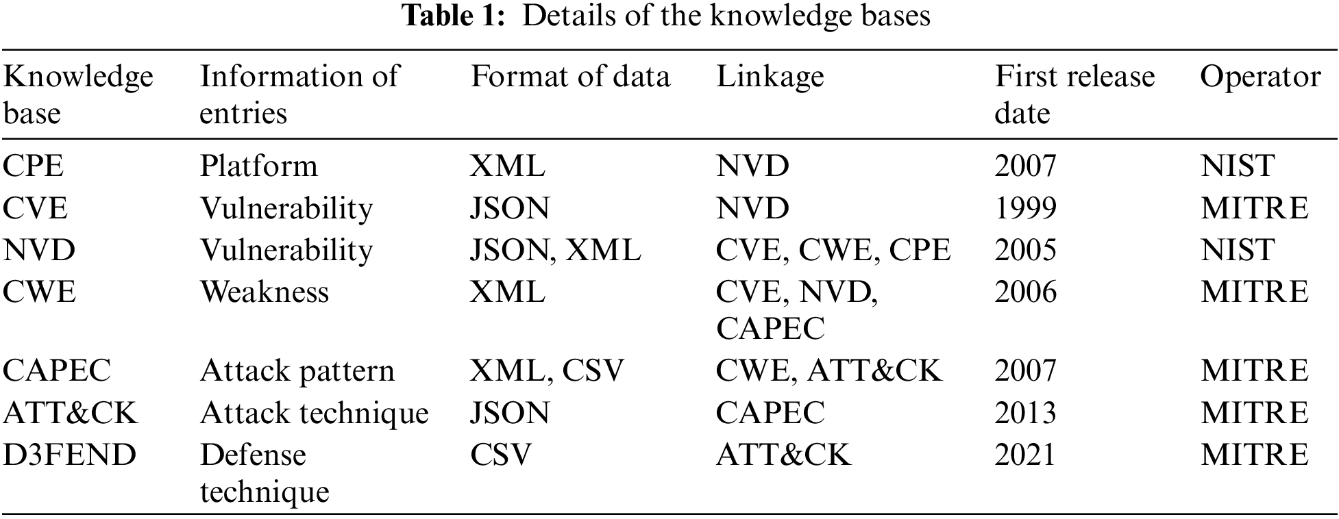
Fig. 1 depicts the relationships between the knowledge bases mentioned above. From these knowledge bases, we extract multi-source network security information and store it in a graph database. In particular, the items in each knowledge base function as nodes in the graph database, while the relational linkages across knowledge bases operate as edges. These edges are not bidirectional between the knowledge bases mentioned above. However, they can be bi-directionally navigated when incorporated into the graph structure. As a result, any node can be used to query the data in any knowledge base.

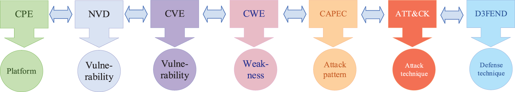
Figure 1: Linkages between knowledge bases

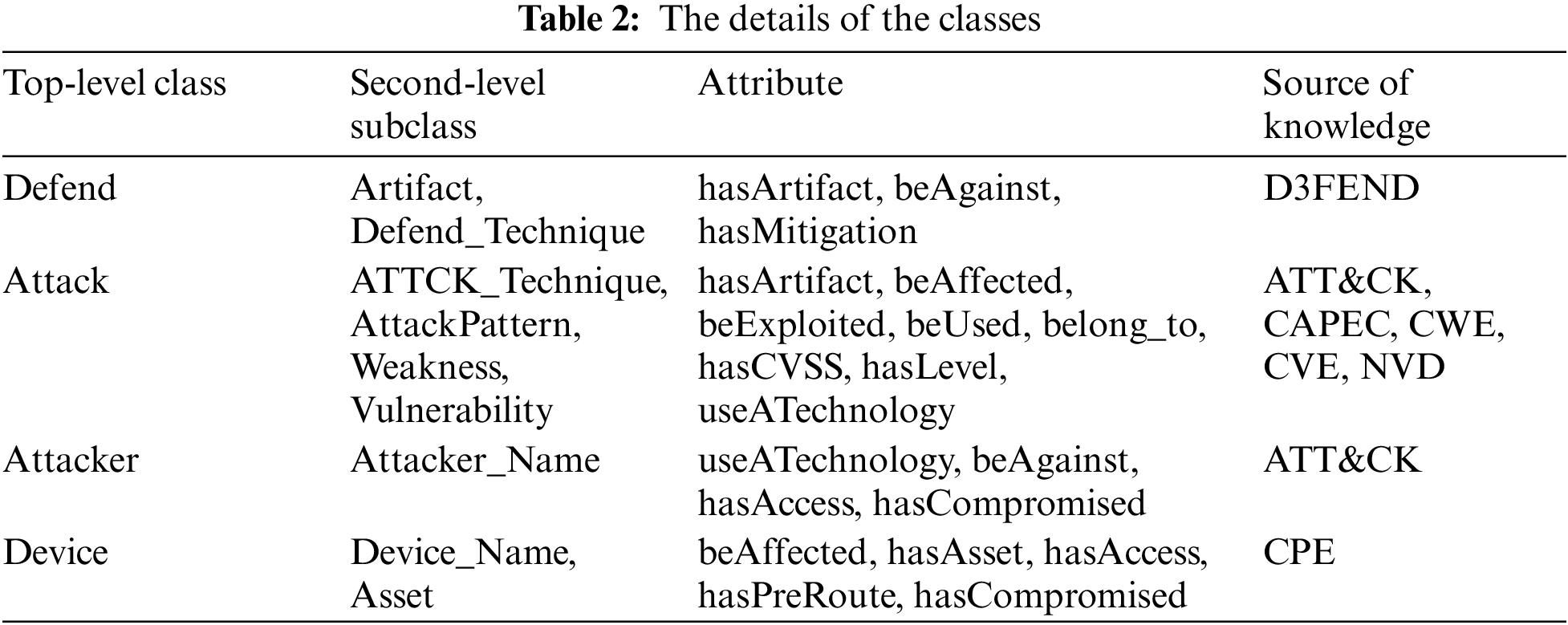
2.2 Classes and Attributes of MTEAO

We successfully linked multiple source knowledge bases and integrated the data from them as a source of security knowledge for developing our ontology model, the multi-source threat element analysis ontology (MTEAO). And we collectively call the entities in it, such as vulnerabilities, weaknesses, attack patterns, attack techniques, defense techniques, etc., as threat elements. The specifics of the MTEAO’s classes are shown in Table 2.

The structure among classes is shown in Fig. 2a, while the logical links among the second-level subclasses are shown in Fig. 2b.

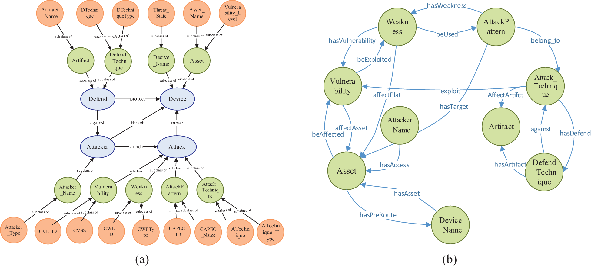
Figure 2: (a) The inclusion relationships among classes; (b) The logical links among the second-level subclasses

2.3 Inference Rules of MTEAO

2.3.1 Design of Inference Rules

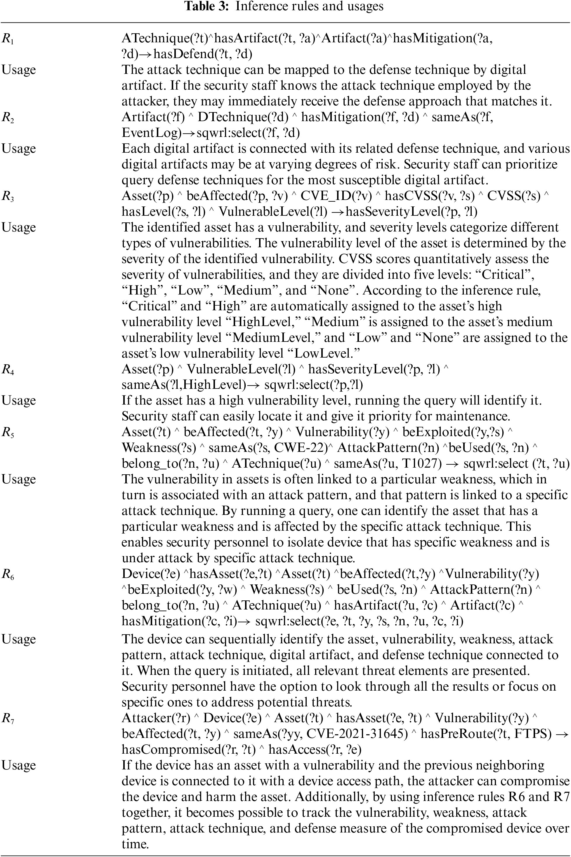
Using inference rules enables us to deduce possible knowledge based on existing information, allowing us to discover new implicit correlations between threat elements. Protégé’s inference engine can execute sequential multi-step inference and aids in comprehending the inferred findings via inference interpretation. Table 3 shows how the seven inference rules in this paper are intended to serve diverse purposes.

2.3.2 Application of Inference Rules

Then, we will demonstrate the practical application of inference rules in combating security threats. Below are two distinct scenarios that will showcase their effectiveness:

1.   Determine the vulnerability level of the asset and whether the asset will be conquered

The asset “arch_newsworld” is stored in the email server and has a vulnerability known as “CVE-2005-3435” with a severity level of “High”. In Fig. 3, the green box shows the vulnerability level of “arch_newsworld” is “HighLevel” by executing inference rule “R3”. Additionally, the officer can use the inference rule “R7” to determine if an attacker can conquer the asset. The red box shows that the attacker can obtain complete control of the email server and compromise the “arch_newsworld” asset.

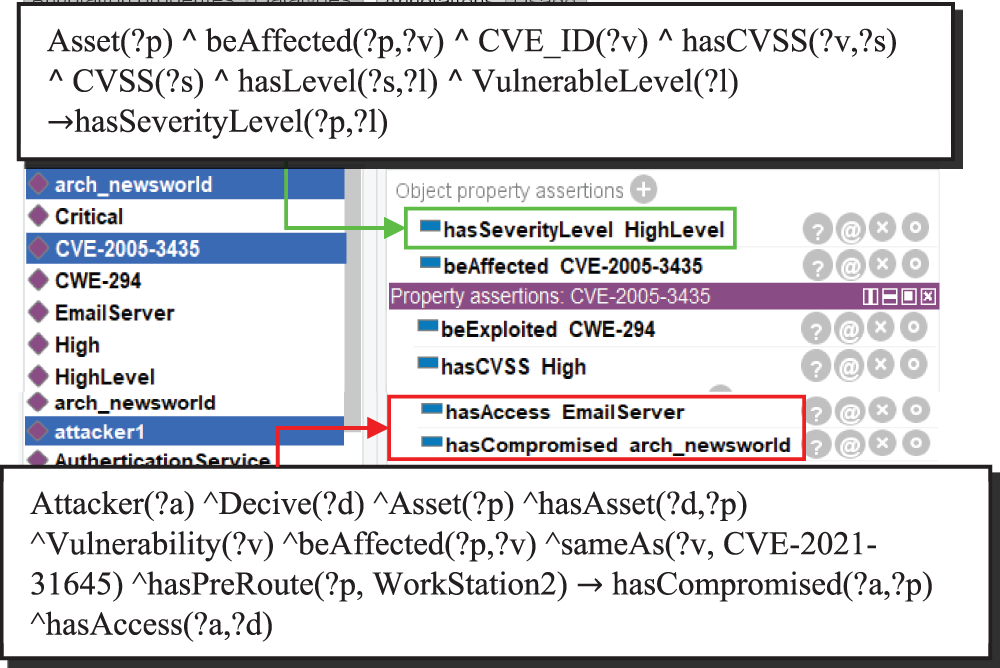
Figure 3: The result of determining the vulnerability level of the asset and whether the asset will be conquered

2.   Search for information on attack and defense

The security officer can execute the “R6” inference rule to retrieve information on devices, assets, vulnerabilities, weaknesses, attack patterns, attack techniques, digital artifacts, and defense techniques. Displayed in the yellow box is the output of utilizing “R6”, as depicted in Fig. 4. The “R1” inference rule can be used by the security officer to search defense techniques that relate to specific attack techniques directly. The green box displays the defense techniques for the attack technique “T1211”.

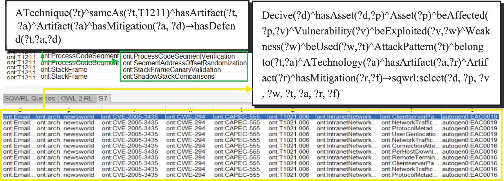
Figure 4: The result of searching for information on attack and defense

3  Two-Layer Threat Prediction Model

In the event of a system threat, the top priority is to address and contain it promptly. As a result, it is crucial to evaluate and forecast the potential progression of the threat. This paper proposes a two-layer threat prediction model called TL-TPM, which aims to enhance the accuracy of predicting attacks. The macro-layer of TL-TPM draws the propagation path of threat between devices and associates these devices with the corresponding threat elements for threat alerting and response; The micro-layer depicts the evolution process of attack techniques while warning of attack techniques with a high probability of use, assisting security personnel to strengthen the prevention of specific attacks. The workflow of this paper is shown in Fig. 5.

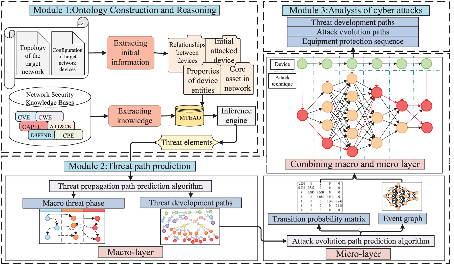
Figure 5: Workflow of the system

3.1 The Macro-Layer of Threat Prediction Based on Knowledge Graph

To accomplish his attack goal, the attacker will exploit weaknesses in the target network and execute a series of consecutive attacks. The macro-layer of TL-TPM maps this set of attack sequences as a propagation path of threat between devices. We describe the concept “attack” in the ontology as a relation link between the attackers and devices, changing the attack path prediction issue into the link prediction issue in the knowledge graph. To aid in the explanation of the below algorithm, the appropriate definitions are provided:

•   Core asset (cas): The target asset the attacker aims to seize or obliterate.

•   Threat degree (thd): The level of risk to the core asset when the device is under attack. The greater the threat level of a device, the more likely it is that an attacker will select that device for the next attack, leading the threat to spread to the core asset. thd ∈ [0, 1].

•   Threat degree interval (tdi): Security personnel determine the interval of threat degree to classify the risk stages according to their needs.

•   Topology layer (tl): The positioning layer of a device in the system topology. The device closer to the core assets is defined as a higher layer.

•   Attack success probability (asp): The success probability of an attacker performing a single-step attack.

•   Device set (Devices): A set of all the devices in the system.

•   Business access relationship (bar): The access and control relationship between two devices. d0→bar1d1→bar2⋯→barndn expresses the business access relationships from device d0 to device dn. And Bar denotes the set of business access relationships.

•   Device access path(dpath): An acyclic series of devices connected by business access relationships. The device access path from the specific device d0 to the core asset located device dn is represented as dpath= {d0,d1,..., dn}.

•   Threat propagation path (tpath): It is an ordered sequence of devices conquered by the attacker.

•   Initial device (ind): The device initially attacked by the attacker.

•   Pre-privilege: It is the pre-condition that a business access relationship exists between device dt and the previous one dt−1.

•   Post-privilege: It is the post-condition that there is a vulnerability in the device, leading the attacker to gain complete control of the device dt by launching an attack.

3.1.1 Calculation of Threat Influence Elements

The role of the attacker’s psychology in the threat spread procedure is overlooked by most existing attack prediction systems. We evaluate the threat degree of the device based on the attack success probability to estimate the threat propagation path, considering that an attacker would always use the most favorable methods to attack the most susceptible device.

1.   Calculation of the Attack Success Probability

Attack success probability refers to the success probability of an attacker performing a single-step attack. Specifically, there are two types of attacks: social engineering attacks and vulnerability exploit attacks. Professional security staff can easily avoid social engineering attacks, so the probability of success is low at 0.2. While the probability of success for vulnerability exploit attacks is determined by the Common Vulnerability Scoring System (CVSS) score [23].

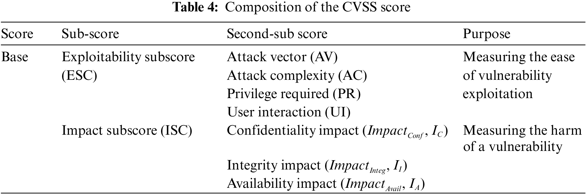
The CVSS score has a base score (Base) that reflects the inherent characteristic of a vulnerability, which remains unchanged over time and environment. The composition of the CVSS score is shown in Table 4. And its calculation formulae are shown in Eqs. (1) and (2).

Base={Roundup(Min[(ESC+ISC),10]),else0,ISC≦0(1)

{ESC=8.22∗AV∗AC∗PR∗UIISC=1−[(1−ImpactConf)×(1−ImpactInteg)×(1−ImpactAvail)](2)

pos=0.1∗Roundup[(Base∗ExploitCodeMaturity)](3)

2.   Calculation of the Threat Degree

If device d0 in the device access path dpath is compromised, the threat degree to the core asset can be calculated in the following way:

i.   When dpath = {d0}, which means that the core asset is present in the initial device of the path, and that device has been compromised, then the threat degree is computed as Eq. (4).

dht(d0, cas)=1(4)

ii.   When dpath≠ {d0}, the attacker can only spread the threat from one device to another by conducting an attack. Therefore, the threat degree of the device can only be determined if the threat propagation path tpath exists on the device access path dpath. If not, it signifies that the threat cannot be disseminated to the core asset via the dpath by attack techniques. As a consequence, the threat degree is 0.

To successfully compromise the high-topology layer device, the low-topology layer device must first be compromised. Consider the ratio of topological layer numbers between the device and the core asset as the weight. A higher weight indicates that device dt is closer to the core asset. In addition, the attacker must take control of every device in the threat propagation path before device dt if he wishes to compromise device dt. So, this weight is then multiplied by the multiplication of the attack success probability of all devices on the threat propagation path passed from the initial device d0 to device dt. In this case, the threat degree is calculated as Eq. (5).

thd(dt,cas)={tldttlcas∗(∏dϵtpathasp(d)),tpath≠∅0, tpath=∅(5)

If device dt has more than one adjacent device, and there is the tpath on the dpath between dt and each adjacent device. Then, the device with the highest threat degree among the adjacent devices is selected as the next target to attack and spread the threat.

3.1.2 Threat Propagation Path Prediction Algorithm

Next, this paper presents the threat propagation path prediction algorithm (TPPPA) based on the knowledge graph. TPPPA not only sequentially strings the attacked device nodes into a path but also associates them with the corresponding multi-source threats elements. It predicts the path while outputting relevant threat information, giving security personnel an intuitive understanding of the attacks being suffered and their countermeasures.

The core code of TPPPA is as follows:

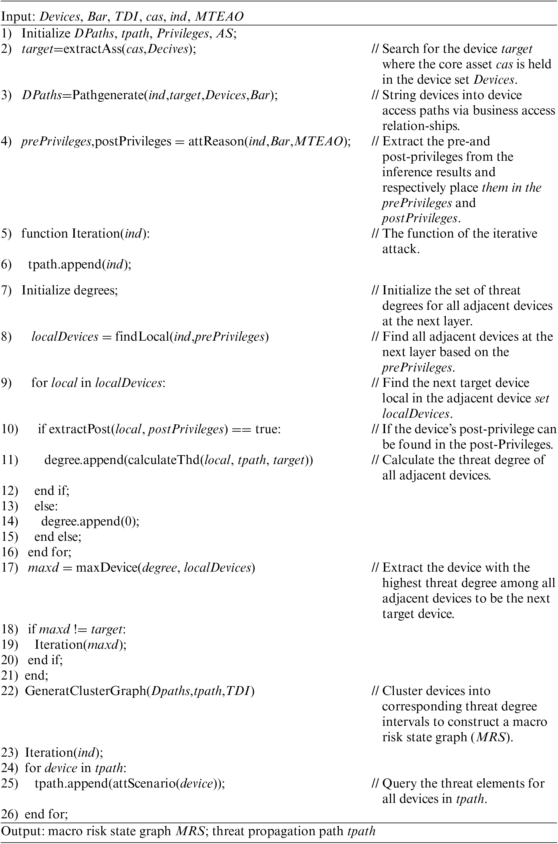
The algorithm described above follows a series of steps: Steps 1)~4) involve initializing the required sets and extracting required data. Steps 5)~21) form the heart of the algorithm, predicting the threat propagation path. Because to completely control the device dt, both requirements must be simultaneously met: 1. The adjacent device dt−1 of device dt had been completely controlled by the attacker. And a device access path exists between the dt−1 and dt. 2. The device dt contains a vulnerability. As a result, the pre-privileges are extracted to establish the device access path and then the post-privileges are extracted to determine whether the threat propagation paths exist. Then, select the device with the highest threat degree among the adjacent devices as the next target. Afterward, create the directed edge to form the complete threat propagation path. Step 22) clusters devices into corresponding threat degree intervals and produces the macro threat state graph. Steps 23) ~26) extract threat elements for all devices in the tpath and presents the result with the knowledge graph.

3.2 The Micro-Layer of Threat Prediction Based on Event Graph

The micro-layer of TL-TPM uses an absorbing Markov chain to map the attack graph to the event graph, which depicts the evolution process of attack techniques. It can warn of attack techniques with a high probability of use, assisting security personnel to strengthen the prevention of specific attacks.

3.2.1 Preliminary Knowledge and Theoretical Arguments

This section first explains the basic concepts of the attack graph and absorbing Markov chain, then argues the rationality of mapping the attack graph to the event graph through the absorbing Markov chain. Finally, the attack evolution path prediction algorithm is presented.

1.   Attack graph

The attack graph (AG) is a visualization method to model the association of multi-step attack behavior and represent the attack process [24]. It is a directed graph that portrays all possible penetration paths of an attacker in the network. An example of an attack graph is shown in Fig. 6.

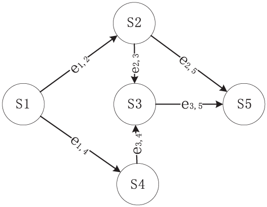
Figure 6: The example of an attack graph

AG is represented by a quadruple AG=(S,E,A,δ), where:

•   S denotes the set of state nodes, S={Si|i=1,2,⋯,j} denotes the set composed of j different state nodes, and the state nodes can be divided into starting state nodes, transition state nodes, and target state nodes. For example, in Fig. 6, S1 is the start state node, S2, S3, S4 are the transition state nodes and S5 is the target state node;

•   E denotes the set of directed edges between state nodes, em,n∈E, em,n represents the edge of the state node Sm pointing to Sn, i.e., a state transfer has occurred from Sm to Sn;

•   A denotes the set of atomic attack nodes, A={ai|i=1,2,⋯,j}, ai is an atomic attack, with each successful attack corresponding to a state transition em,n.

•   δ denotes the set of state transition probabilities, δ(em,n) denotes the probability P(Sm|Sn) of the attacker transferring from state Sm to state Sn, and δ(em,n) is equal to the probability P(a) of an atomic attack a occurring.

2.   Absorbing Markov chain.

The main advantages of Markov processes are the ability to build prediction models in time based on statistical information or the results of operational observations [25]. And the Markov chain (MC) is a Markov process in which both time and state are discrete [26]. For a discrete set S={s1,s2,⋯,sn} containing a finite number of states, each state is only related to the previous adjacent state, called posteriority-free, i.e., P(si|si−1,si−2,⋯s1)=P(si|si−1). The probability P(si|si−1) is the transition probability of the state si→si−1, and the transition probabilities between all state nodes form the state transition probability matrix P.

The absorbing Markov chain (AMC) is an MC that contains at least one absorbing state and from which any one of the states can eventually reach the absorbing state. If an AMC has r absorbing states, t non-absorbing states, and all states are n, then n=r+t. At this point, the state transition probability matrix is expressed as P=[QR0I]. Q is the t×t matrix representing the probabilities of transition between transition states; 0 is the r×t zero matrix; R is the t × r non-zero matrix representing the transition probabilities from transition states to absorbing states; and I is the r×r unit matrix.

3.   Mapping of attack graph to the absorbing Markov chain

In AG, the transition of the current state si to the next state si+1 is only related to whether the state si satisfies the vulnerability exploitation, independent of the previous states, at which point the transition between states is precisely in line with the posteriority-free property of MC; The attacker will eventually reach a stable termination state through a multi-step attack based on vulnerability exploitation, which is consistent with the absorption state of AMC; A network attack has at least one termination state, and an AMC has at least one absorbing state; And the successful probability of atomic attack in AG can be regarded as the state transition probability in AMC. Therefore, AG can be mapped to AMC.

4.   Mapping of absorbing Markov chain to event graph

The event graph (EG) represents events and their relationships as a logically directed graph. It takes abstract and generalized events as nodes, connected to form directed edges that express the evolution process between events. And this process can be considered as a transition between events, then the transition probability on the directed edge represents the probability of the event’s evolution. This probability can be calculated and expressed precisely in terms of the transition matrix of AMC. Thus, AMC can be mapped to the EG. At the same time, we can optimize the Markov transition matrix by considering multiple dimensions affecting the event transition and assigning different weights to them. So far, we have achieved the mapping from AG to EG.

3.2.2 Attack Evolution Path Prediction Algorithm

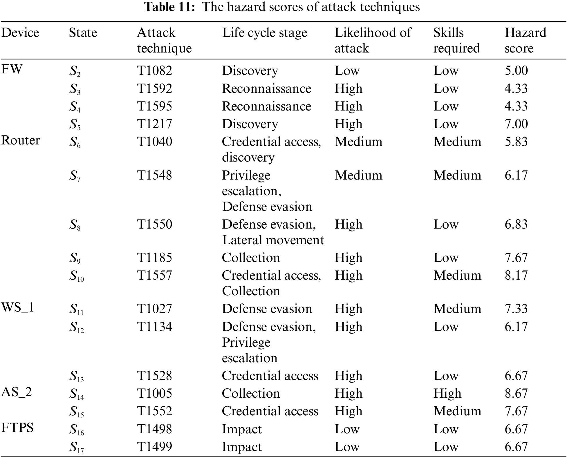
Unlike the way of calculating event transition probability in general EG, this paper optimizes it to reflect the event evolution process better. We propose an available method for measuring the hazard of an attack technique. We calculate the hazard of attack techniques from three metrics: “Life Cycle Stage”, “Likelihood of Attack”, and “Skills Required0”. The higher hazard means the higher the probability that the attacker will use the attack technique, then the higher the likelihood that the attack technique will transfer.

The ATT&CK matrix contains 14 attack strategies, and each attack strategy includes several attack techniques. It represents a complete sequence of attack lifecycle stages in the form of a table from left to right. The further back the attack technique is in the lifecycle stage, the closer it is to complete an attack and the more harmful it is. Therefore, each attack technique is scored according to the attack lifecycle stage it belongs to.

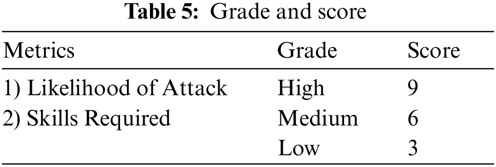
The two metrics in CAPEC are: “Likelihood of Attack” and “Skills Required”. Both metrics measure the probability of an attack occurring and are graded as “High”, “Medium”, and “Low”. As shown in Table 5, we converted them into scores “9,” “6”, and “3” to quantify the probability of using the attack technique. The higher the probability that an attack technique is used, the more harmful it is.

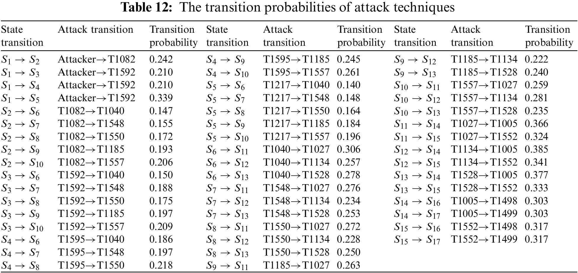
Each attack technique is scored on the above three metrics, and the three scores are summed and averaged for the final attack technique hazard score. Based on the method of attack technique hazard metric, we propose the attack evolution path prediction algorithm (AEPPA). AEPPA normalizes the attack technique hazard score to realize the mapping from AG to AMC and finally constructs the EG with the Markov transition matrix. The core code of AEPPA is as follows:

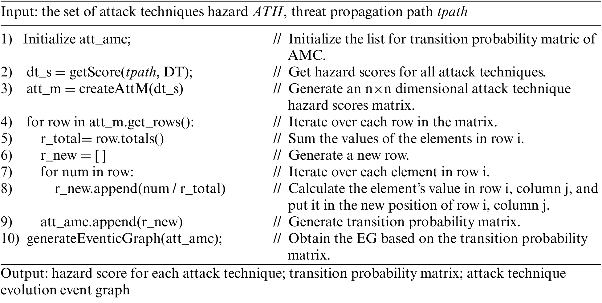
The algorithm described above follows a series of steps: Step (1) initializes the list for transition probability matric of AMC. Step (2) uses the method of attack technique hazard metric to obtain the hazard scores for all attack techniques based on the set of attack techniques hazards. Step (3) generates an n × n dimensional matrix using the hazard scores of all attack techniques. If the attacker and the attack techniques are considered state nodes, then n represents the number of state nodes, and the values of rowi represents the score from the statenodei to all state nodes. Steps (4) ~ Step (9) calculate and obtain the transition probability of each attack technique to itself and any other attack technique, and put them into the matrix list in Step (1). At this point, we obtain the transition probability matrix of AMC. Step (10) gets the EG based on the transition probability matrix.

AEPPA finally outputs the hazard score for each attack technique and the transition probability matrix of the attack techniques, enabling the subsequent analysis of the evolution process to depend on accurate data. At the same time, the visualization of EG enhances the understanding of the evolution process of threat events.

4  Experiment

4.1 Scene of the Experiment

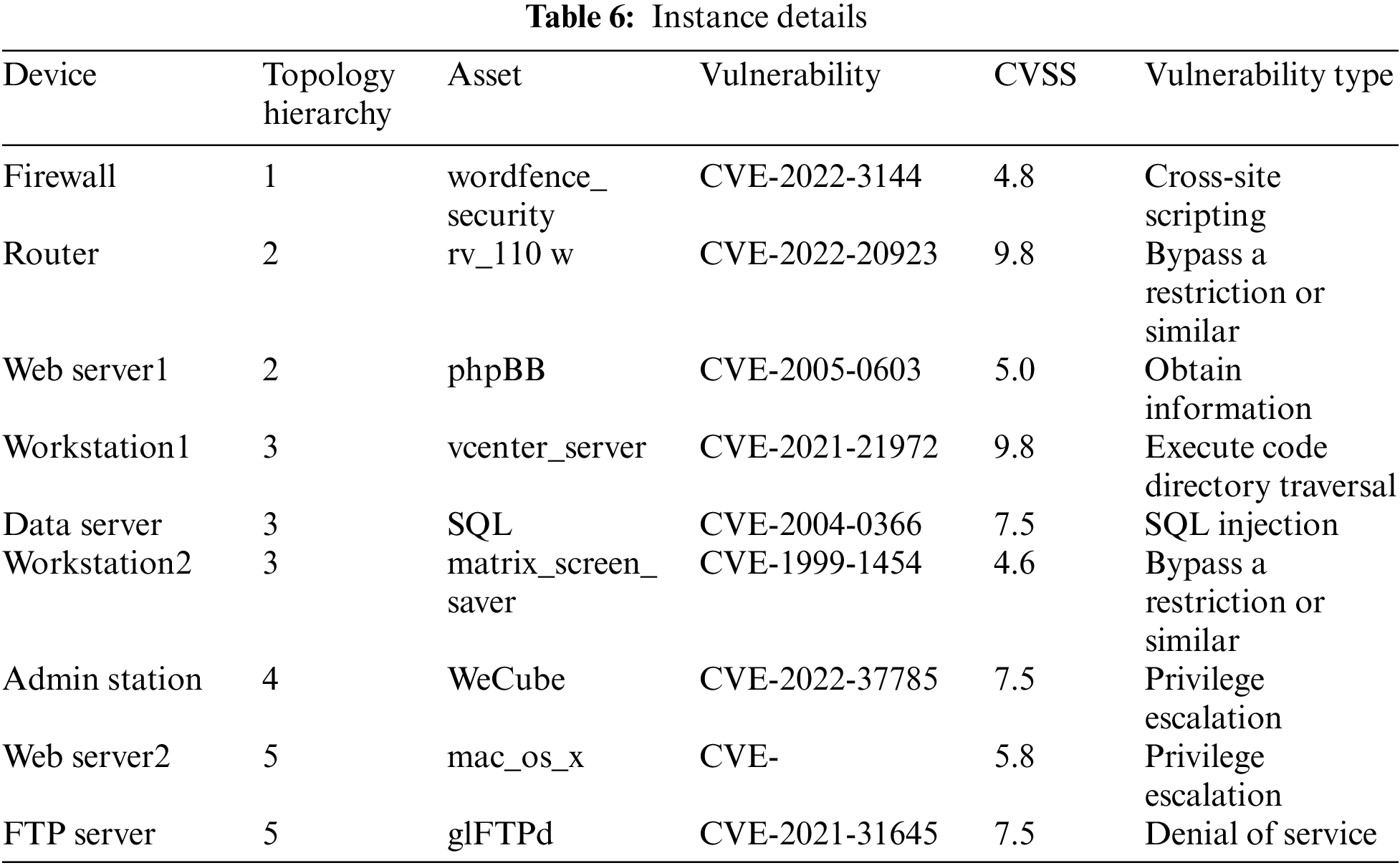
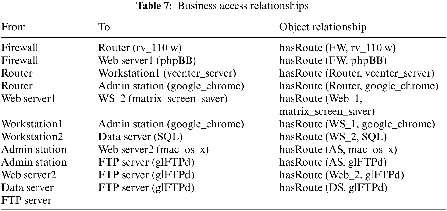
The experiment scene is shown in Fig. 7. The system consists of three subnets, with a firewall and the intrusion detection systems (IDS) deployed to achieve access control and intrusion detection. The firewall allows only the workstation and web server in the demilitarized zone (DMZ) to interact with the outside world, and the network line of the workstation1 is connected from the router; Subnet 1 deploys an administration station, a web server, and a file transfer protocol server. And the router also connects with the administration station, which can interact with workstation1 and access the web server2 and file transfer protocol server; Subnet 2 deploys a workstation and a data server. Web server1 and workstation2 have user accounts of the data server and can access the data server. Tables 6 and 7 present the corresponding information and the business access relationships of the devices in the system.

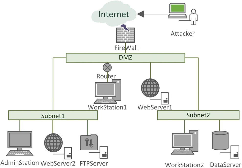
Figure 7: Scene of the experiment

4.2 Threat Prediction

The following initial conditions are given in Table 8 according to the experiment scene. In this section, predictions are respectively made at the macro-layer and micro-layer.

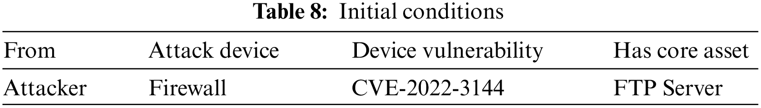
4.2.1 Macro Threat Prediction Experiment Based on Knowledge Graph

Based on the threat degrees of the devices, users can set the appropriate threat degree intervals according to their needs to divide the threat status stages and cluster devices with the same threat degree in the same interval. Assume that the enterprise stipulates that the threat degree does not exceed 0.15 is low-risk status, 0.15 to 0.20 is medium-risk status, and over 0.20 is high-risk status. And the three risk states of low, medium, and high are respectively marked with blue, yellow, and red colors. Executing the TPPPA based on the initial conditions, the macro risk state graph is constructed as shown in Fig. 8. The circles in Fig. 8 represent the devices under attack; the dotted links constitute the device access paths; and the solid links form the threat propagation path, indicating the actual trajectory of the threat as it moves from the low threat degree devices to the high threat degree devices. The threat degree and vulnerability type of each device is shown in the rectangular box. For simplicity of expression, the devices are replaced by abbreviations, e.g., the firewall is written as FW.

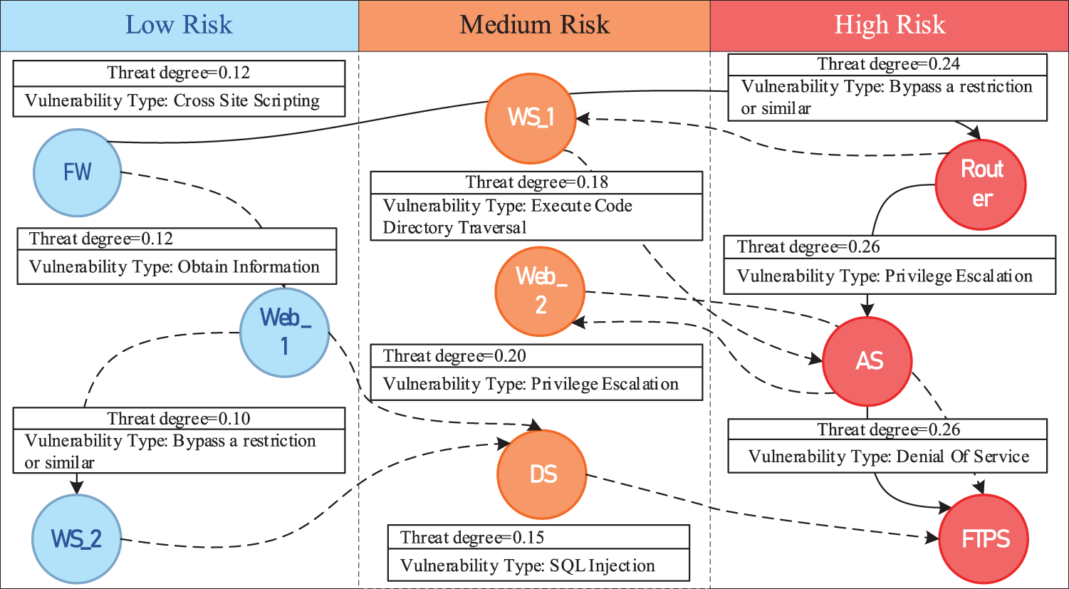
Figure 8: Macro risk state graph

At the same time, TPPPA calculates the devices most likely to be compromised by the attacker at each step, links them sequentially into the path, and connects them to the associated multi-source threat elements for a complete threat propagation path graph. The threat propagation path is marked with black arrows in Fig. 9, and the different colored circles represent different threat elements. Security personnel can rely on the graph to quickly grasp the threat and take appropriate defensive measures for each attack to contain the spread of the threat.

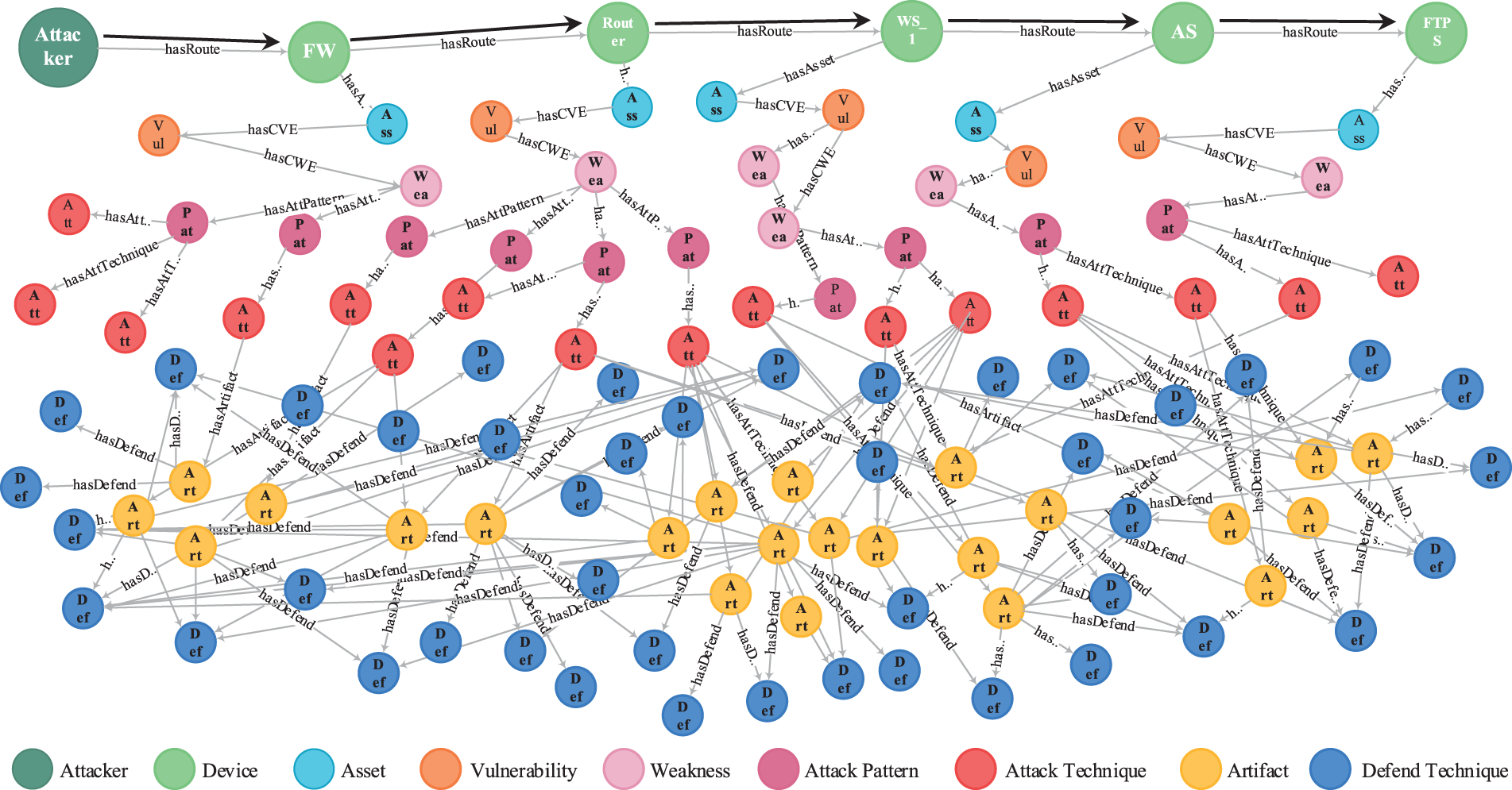
Figure 9: Threat propagation path and threat elements

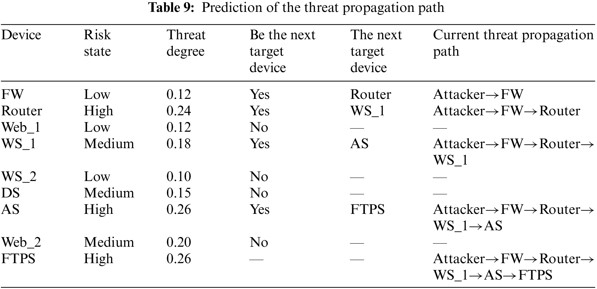
Based on the experiment results, the attacker’s intent was analyzed as follows:

1.    The attacker conquered Firewall (FW) by attacking the vulnerability “CVE-2022-3144” in the software “Wordfence_Security”, which caused FW to be injected malicious web scripts into the settings and to be compromised completely.

2.    Then, the attacker attacked the Router by exploiting the vulnerability “CVE-2022-20923” in hardware “rv_110w”, which allowed the unauthenticated attacker to bypass authentication.

3.    Since Work Station 1 (WS_1) was connected from the Router and its server management software “vcenter_server” contained a remote code execution vulnerability “CVE-2021-21972”. The attacker used CVE-2021-21972 to execute commands with unrestricted privileges and thus gained complete control of WS_1.

4.    There was a business access path between WS_1 and the Admin Station (AS), and the attacker attacked the AS along the network. AS owned the software “WeCube”, which contained the vulnerability “CVE-2022-37785” that caused plaintext passwords to be displayed in the terminal plug-in configuration. The attacker then exploited the vulnerability to steal passwords and gain complete control of AS.

5.    Via AS, the attacker accessed the FTP Server (FTPS), where the core asset is located. The FTPS contained the software “glFTPd” with the vulnerability “CVE-2021-31645”. By breaking the link limit with CVE-2021-31645, the attacker triggered a threat of denial service.

Combined with the macro risk state graph, the experiment results were compiled to present the corresponding prediction information, as shown in Table 9.

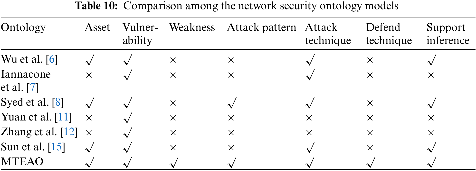
Through the above analysis, the attack steps can be visualized, and the predicted threat propagation path can be used to contain the threat spread in time, which proves the effectiveness and practicality of TPPPA. While TPPPA is based on the ontology model MTEAO, this ontology model extends and improves the modeling knowledge of the security domain compared to the previous work. In Table 10, the MTEAO is compared to other ontology models, and the results are presented below:

4.2.2 Micro Threat Prediction Experiment Based on Event Graph

Based on the prediction results of the threat propagation path in Experiment 4.2.1 and executing AEPPA, the attack technique hazard scores of the devices, the Markov transition probability matrix, and the attack technique evolution event graph are obtained to deepen the prediction.

AEPPA first takes the path predicted by TPPPA as input and outputs the state transition matrices P and Q, then calculates the matrix N according to the formula N=(I−Q)−1. The matrix N represents the expected number distribution of state node visits. The values in the first row of it are the number of visits from the state node S1 to each remaining state node. In the context of the experiment in this paper, the values in the first row of the matrix N can be interpreted as the number of times the attacker uses each attack technique. And the higher the number of times the attack technique is used, the higher the probability of its use. Matrices P, Q, and N are shown below. Tables 11 and 12 give information about the attack techniques based on the results returned by TEPPA.

P=[00.2420.2100.2100.33900000000000000.1260000.1470.1550.1720.1930.2060000000000.111000.1500.1580.1750.1970.20900000000000.13800.1860.1970.2180.2450.261000000000000.1680.1400.1480.1640.1840.1960000000000000.22400000.3060.2570.27800000000000.2340000.2780.2340.253000000000000.253000.2720.2280.2500000000000000.27500.2630.2220.24000000000000000.2880.2590.2180.235000000000000000.310000.3660.32400000000000000.27400.3850.341000000000000000.2900.3770.3330000000000000000.39400.3030.303000000000000000.3650.3170.3170000000000000001000000000000000001]

Q=[00.2420.2100.2100.339000000000000.1260000.1470.1550.1720.1930.20600000000.111000.1500.1580.1750.1970.209000000000.13800.1860.1970.2180.2450.2610000000000.1680.1400.1480.1640.1840.19600000000000.22400000.3060.2570.278000000000.2340000.2780.2340.2530000000000.253000.2720.2280.25000000000000.27500.2630.2220.240000000000000.2880.2590.2180.2350000000000000.310000.3660.324000000000000.27400.3850.3410000000000000.2900.3770.33300000000000000.3940000000000000000.365]

N=[1.0000.2770.2360.2440.4070.2300.2460.2800.3240.3510.5660.4530.5020.9420.79501.1440000.2170.2320.2630.3050.3310.5340.4270.4730.8870.749001.125000.2170.2320.2640.3060.3300.5340.4270.4730.8880.7500001.1600.2780.2980.3390.3920.4250.6860.5480.6081.1410.96300001.2020.2170.2320.2640.3050.3310.5340.4270.4730.8880.750000001.28900000.5710.4560.5050.9490.8010000001.3050000.5260.4210.4650.8740.73800000001.339000.5280.4200.4710.8790.742000000001.37900.5260.4220.4660.8760.7390000000001.4040.5270.4220.4660.8760.73900000000001.449000.8750.739000000000001.37700.8750.7400000000000001.4080.8760.73900000000000001.6500000000000000001.575]

TEPPA first links the attack techniques into the AG, constructs the AMC based on the AG, and then maps the AMC to the EG. Fig. 10 shows the AG and the mapped attack technique evolution event graph, where the state transition probabilities on the edges have been normalized.

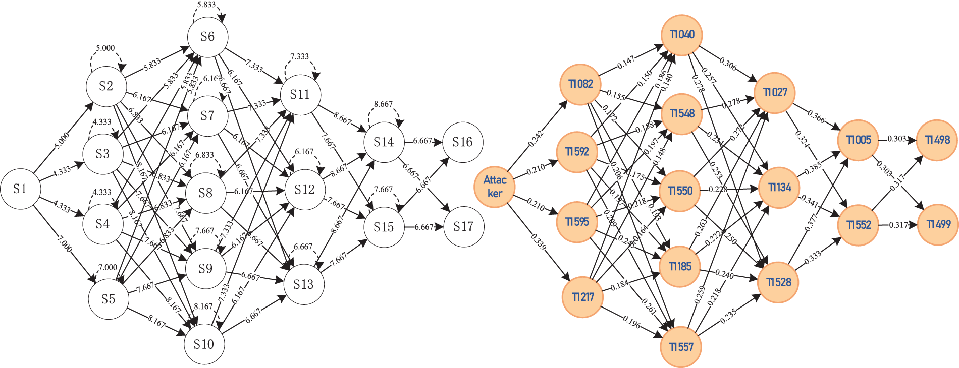
Figure 10: Mapping of attack graph to attack technique evolution event graph

In Fig. 11, the red circles indicate the attack techniques with the highest probability of being used to compromise each device. They are connected by red lines to form the attack technique evolution path with the highest probability. Finally, we integrate the prediction results from the macro and micro-layer, which enables the mapping of the attacked devices to the attack techniques. Security personnel can visualize the most likely attack paths and techniques attackers use to protect critical devices and prevent specific attack techniques better.

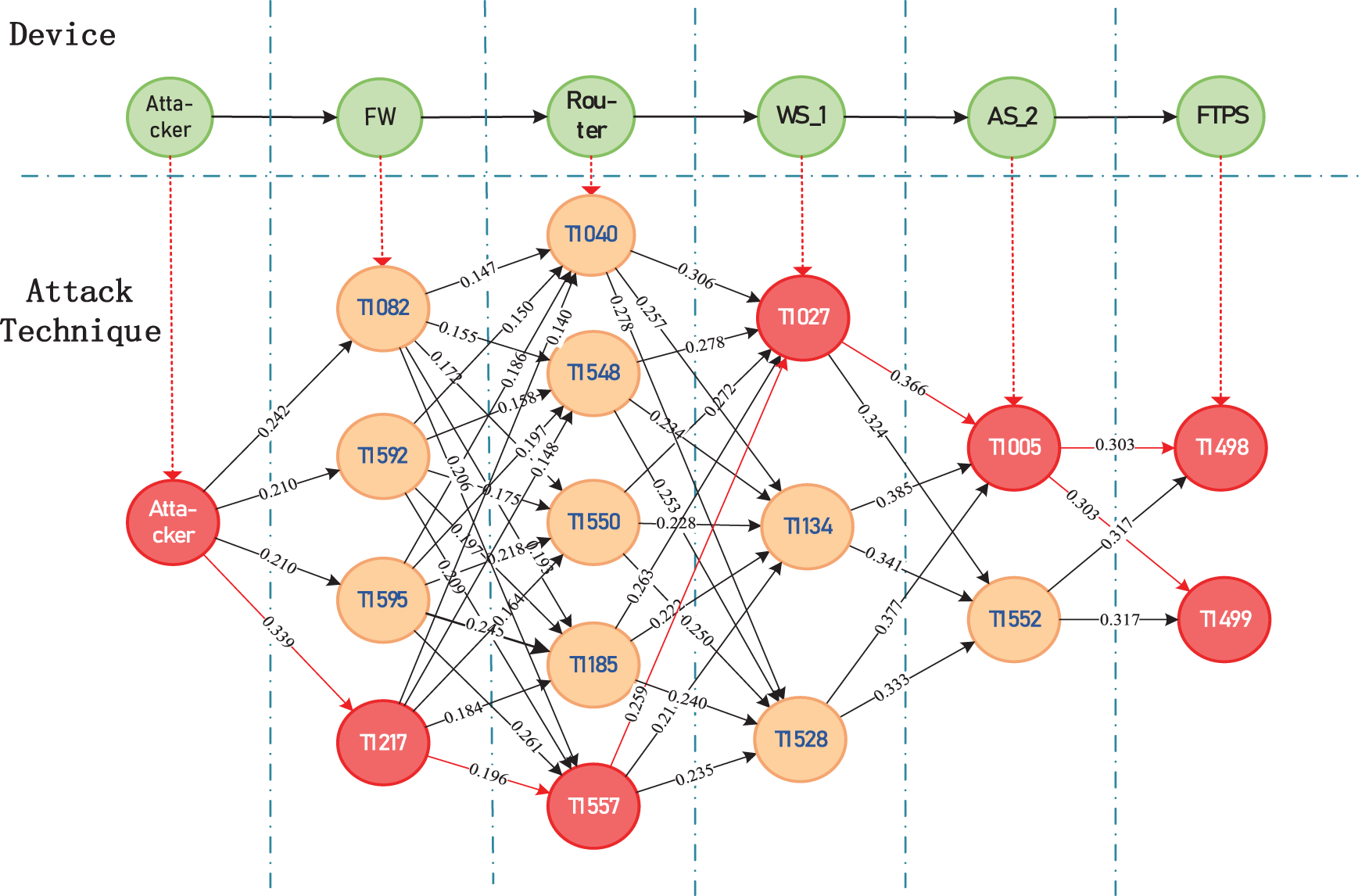
Figure 11: TL-TPM combines macro and micro-layer

A device can be attacked by more than one attack technique, so when the probabilities of all possible attack techniques are summed, the higher the value, the higher the probability of the device being attacked. We regard this probability as the hazard degree of the device and determine the protection sequence of the device according to the hazard degree. In summary, the protection sequence of the device in the threat propagation path can be predicted based on the matrix N. As seen in Fig. 12, FW, Router, WS_1, and AS are the devices in the threat propagation path predicted by TPPPA. S2–S15, respectively, correspond to an attack technique, clustered according to the attacked device FW, Router, WS_1, and AS. The bar chart shows the number of visits to each attack technique, which represents the use probability of it. The line in the graph shows the sum of the use probabilities of all attack techniques for each device, i.e., the risk degree of the device.

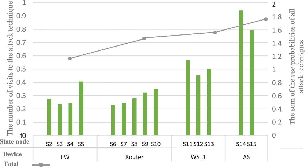
Figure 12: Expected number distribution of using each attack technique

The higher the risk degree of the device, the higher the priority to protect it. Therefore, from the line in Fig. 12, we can see that the sequence of device protection in the threat propagation path predicted by AEPPA is: AS>WS_1>Router>FW. Meanwhile, the attack technique T1005, represented by the state node S14, has the highest number of node visits. It indicates that the attacker will most likely use T1005, so AS should be strengthened to defend T1005.

4.3 Contrast Analysis

In this section, to illustrate the effectiveness of TL-TPM, this paper compares it with Hu et al.’s [10] model. Specifically, TL-TPM compares the prediction results of the device repair sequence and threat propagation path, and the time complexity. Finally, it compares with several previous models in a comprehensive way.

1.   Prediction of Device Repair Sequence

We use Hu Hao’s method to obtain his device repair sequence for this experiment scene. The topology of the experiment scenario is shown in Fig. 13. Similarly, his method needs to derive the state transition probability matrices P’ and N’, and the values in the first row of the matrix N′ are used to determine the sequence of repair. The matrices P’ and N’ are shown below.

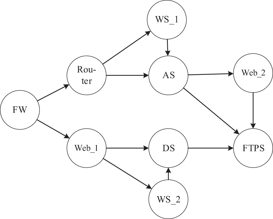
Figure 13: The topology of the experiment scenario

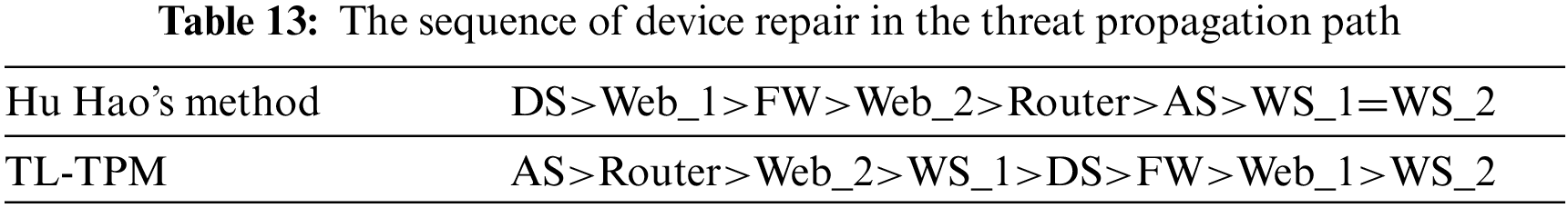
To illustrate the effectiveness and superiority of TL-TPM, we compare the predicted outcomes of device repair sequences of TL-TPM with Hu Hao’s method. Table 13 illustrates the device repair sequences, and it can be observed that Hu Hao’s method indicates that DS should be prioritized for repair when adopting network security measures, but TL-TPM indicates that AS should be prioritized for repair.

P′=[01.0000000000000.1090.6410000.250000000.4180.1630.418000000000.2800.7190000000000.71900000.280000000.3330.3330.333000000000.23800.5240.2380000000.5000.50000000000000.6880.3120000000001]N′=[1.0001.1221.2360.2802.5550.4210.3680.2800.61701.1221.2360.2802.5550.4210.3680.2800.617001.7180.3893.55100000001.3893.554000000003.5590000000001.4991.310.9992.2010000001.31202.2040000001.31222.204000000003.205]

For this discrepancy, we analyze the effect of device node repair. Repairing a device node, i.e., deleting it and all edges associated with it in the topology graph, and then counting the number of remaining attack paths, the results are shown in Fig. 14. And from Fig. 13, it can be found that there are six attack paths that can attack FTPS. It is clear that when priority is given to protecting AS, i.e., the device node is removed from the graph, and the remaining attack paths are two. While the DS is removed, the remaining attack paths are four. Therefore, the result of TL-TPM is more scientific and accurate. If the device nodes are repaired sequentially according to the repair sequence in Table 13, it can be seen from Fig. 15 that both Hu Hao’s method and TL-TPM leave only two attack paths after repairing the device for the third time, and leave no attack paths after repairing the device for the fourth time. But TL-TPM overall outperforms Hu Hao’s approach by intercepting more attack paths earlier.

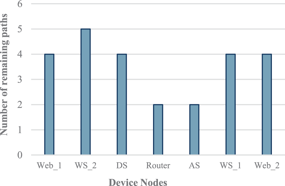
Figure 14: The number of remaining paths after node repair

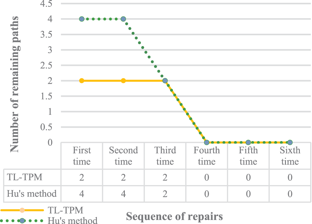
Figure 15: The remaining attack paths after repairing devices in sequence

2.   Prediction of Threat Propagation Path

Next, we compare the threat propagation path predicted by TL-TPM and Hu Hao’s method. Hu Hao’s model first obtains the state transition probability of each device node according to P′, then the state transition probabilities of the device nodes in each attack path are cumulatively multiplied to calculate the probability of success in compromising the core asset along that path. The path with the highest probability of success is used as the final predicted threat propagation path. The lengths of all threat propagation paths and their success probabilities are shown in Table 14.

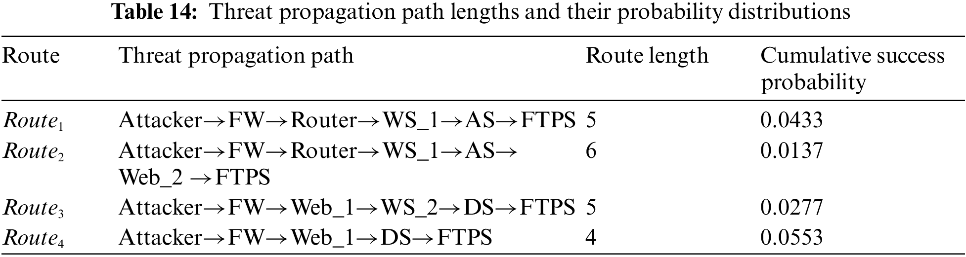
The results in the Table 14 show that Route4 has the highest probability of success. Therefore, the path predicted by Hu Hao’s algorithm is Route4. And as seen from the previous section, the path predicted by TL-TPM is Route1, which differs significantly from the path Route4 indicated by Hu Hao. This is because Hu Hao’s method multiplied cumulatively the transition probabilities between all devices in the path and simply chose the path with the highest cumulative success probability value, not considering that the attacker penetrated gradually. When the attacker is faced with two attackable devices, he always selects the device that is more favorable to him, i.e., the one with the higher risk degree, to attack. As shown in Table 14, although Route4 has a higher cumulative success probability than Route1, the risk degree of Router in Route1 is higher than that of Web_1 in Route4. As a result, the attacker is more likely to choose Router to attack and follow the Route1. Overall, TL-TPM takes a comprehensive view from the attacker’s point to reflect the actual situation more accurately.

3.   Comparison of Time Complexity

Then, we compare the time complexity of TL-TPM with that of Hu Hao’s model. TL-TPM includes two layers, each containing one main algorithm.

Firstly, the time complexity of TPPPA in the macro-layer is analyzed. According to the algorithm logic, assuming that there are n devices between the initial device ind and the device target where the core asset is located. And the average number of adjacent devices at the next layer for each device is m. Then a total of (n−1)m devices need to be calculated for the threat degree from the ind to the target. So, the time complexity of execution from ind to target is O((n−1)m). Because m is constant, the time complexity of the algorithm is O(n).

Secondly, the time complexity of AEPPA in the micro-layer is analyzed. Executing AEPPA is based on the result of TPPPA. Assuming a total of n attack techniques are extracted from the result, calculating their state transition probabilities requires the generation of two matrices with a time complexity of O(n2). Therefore, the time complexity of TL-TPM to obtain the final prediction result is O(n2) + O(n), i.e., O(n2), while the time complexity of Hao Hu’s model is O(n3). As a result, TL-TPM is superior in terms of time complexity.

4.   Comparison of Other Prediction Models

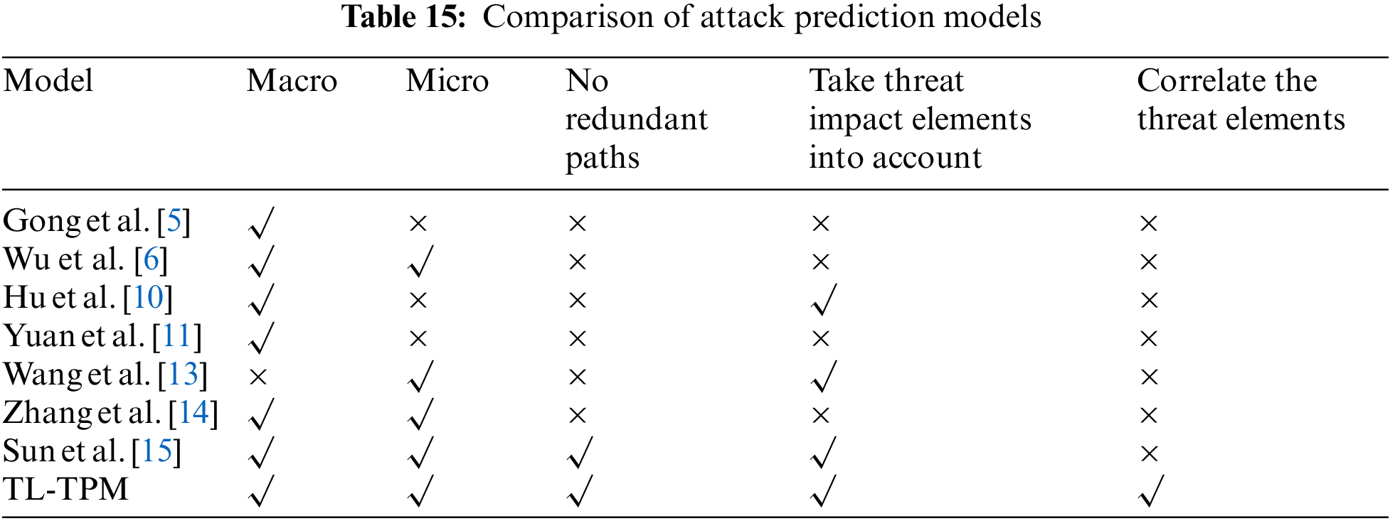
Comparing TL-TPM with other attack prediction models, the results in Table 15 show that TL-TPM is more advanced with considering both macro and micro-layers to predict threat development. It considers the threat impact elements (attack success probability, threat degree) and avoids path redundancy. Furthermore, only this paper’s research has the capability of predicting the threat propagation path while correlating the attacked devices with their respective threat elements, broadening the range of predictions. Moreover, TL-TPM can accurately predict the attack techniques, not only letting security personnel know which devices should be protected in priority but also which attack techniques should be strengthened against.

5  Conclusion

Unlike most previous works that predict the attack based on only one layer, this paper proposes a two-layer model TL-TPM that predicts the development trend of threat events from both macro and micro-layers. The macro-layer proposes the threat propagation path prediction algorithm TPPPA based on the knowledge graph. TPPPA measures the device threat degree by combining system topology and attack success probability. Based on the device threat degree, it predicts the devices under attack, then links them sequentially into threat propagation path and correlates each device with relevant threat elements, which provides decision support for defense response. The micro-layer proposes the attack evolution path prediction algorithm AEPPA based on the event graph. AEPPA combines the prediction results of the macro-layer with the temporal characteristics of the attack behaviors and innovatively maps the attack graph to the event graph using the absorbing Markov chain as a bridge, which accurately portrays the evolution of the attack techniques used in threat events. Finally, the macro-layer and micro-layer prediction results are integrated to visualize the external path and internal logic of threat event development, enabling security personnel to quickly grasp the threat status of system devices and focus on defense.

However, TL-TPM does not consider zero-day vulnerabilities when predicting threats, and the current algorithms and inference rules only work with known vulnerabilities. For future work, we will use the relationship paths linking attacker entities to target entities in the knowledge graph as features and construct attack samples using historical attack data for the given system. Then, we use machine learning to learn the path features in the attack samples to distinguish the zero-day vulnerabilities from the known vulnerabilities. Meanwhile, TL-TPL does not consider the vulnerability lifecycle, which may affect the calculation of the attack success probability. As a result, we will take the vulnerability lifecycle into account, quantitatively analyze the change in vulnerability exploitability over time, optimizing the calculation of the state transition matrix.

Acknowledgement: The authors would like to thank the reviewers for the correct and concise recommendations that help present the materials better.

Funding Statement: The authors received no specific funding for this study.

Author Contributions: The authors confirm contribution to the paper as follows: methodology: Shuqin Zhang; conceptualization: Shuqin Zhang, Xinyu Su; investigation: Yunfei Han; data curation: Peiyu Shi; analysis and interpretation of results: Yunfei Han, Tianhui Du; validation: Tianhui Du; draft manuscript preparation: Xinyu Su. The authors declare that they have no conflicts of interest to report regarding the present study.

Availability of Data and Materials: The ontology and data can be obtained by contacting the corresponding author.

Conflicts of Interest: The authors declare that they have no conflicts of interest to report regarding the present study.

References

1. J. Zhao, Q. Yan, J. Li, M. Shao, Z. He et al., “TIMiner: Automatically extracting and analyzing categorized cyber threat intelligence from social data,” Computers & Security, vol. 95, pp. 101867, 2020. [Google Scholar]

2. J. Zhao, Q. Yan, X. Liu, B. H. Li and G. Zuo, “Cyber threat intelligence modeling based on heterogeneous graph convolutional network,” in Proc. of the 23rd Int. Symp. on Research in Attacks, Intrusions and Defenses (RAID 2020), San Sebastian, Spain, pp. 241–256, 2020. [Google Scholar]

3. G. X. Xu, M. X. Hu and C. Ma, “Secure and smart autonomous multi-robot systems for opinion spammer detection,” Information Sciences, vol. 576, pp. 681–693, 2021. [Google Scholar]

4. J. Zhao, M. L. Shao, H. Wang, X. M. Yu, B. Li et al., “Cyber threat prediction using dynamic heterogeneous graph learning,” Knowledge-Based Systems, vol. 240, pp. 108086, 2022. [Google Scholar]

5. L. Gong, R. B. Si and Y. Tian, “Research on key technologies of ontology based threat modeling for cyber range,” Journal of CAEIT, vol. 15, no. 12, pp. 1139–1144, 2020 (In Chinese). [Google Scholar]

6. S. Y. Wu, Y. Zhang and W. Cao, “Network security assessment using a semantic reasoning and graph based approach,” Computers & Electrical Engineering, vol. 64, pp. 96–109, 2017. [Google Scholar]

7. M. Iannacone, S. Bohn, G. Nakamura, J. Gerth, K. Huffer et al., “Developing an ontology for cyber security knowledge graphs,” in Proc. of the 10th Annual Cyber and Information Security Research Conf., New York, NY, USA: Association for Computing Machinery, pp. 1–4, 2015. [Google Scholar]

8. Z. Syed, A. Padia and T. Finin, “UCO: A unified cybersecurity ontology,” in Workshops at the Thirtieth AAAI Conf. on Artificial Intelligence, Vancouver, British Columbia, Canada, pp. 195–202, 2016. [Google Scholar]

9. J. Zhao, X. D. Liu, Q. B. Yan, B. Li, M. L. Shao et al., “Automatically predicting cyber attack preference with attributed heterogeneous attention networks and transductive learning,” Computers & Security, vol. 102, pp. 102152, 2021. [Google Scholar]

10. H. Hu, Y. L. Liu, H. Q. Zhang, Y. J. Yang and R. G. Ye, “Route prediction method for network intrusion using absorbing Markov chain,” Journal of Computer Research and Development, vol. 55, pp. 831–845, 2018. [Google Scholar]

11. B. T. Yuan, Z. L. Pan, F. Shi and Z. H. Li, “An attack path generation methods based on graph database,” in IEEE 4th Information Technology, Networking, Electronic and Automation Control Conf. (ITNEC), Chongqing, China, pp. 1905–1910, 2020. [Google Scholar]

12. K. Zhang and J. J. Liu, “A threat path generation method based on knowledge graph,” Computer Simulation, vol. 39, no. 4, pp. 350–356, 2022. [Google Scholar]

13. S. Wang, G. M. Tang and G. Kou, “Attack path prediction method based on causal knowledge net,” Journal on Communications, vol. 37, pp. 188–198, 2016. [Google Scholar]

14. X. Zhang, S. G. Huang, Y. Xia and S. H. Song, “Attack graph-based method for vulnerability risk evalution,” Application Research of Computers, vol. 27, no. 1, pp. 278–280, 2010. [Google Scholar]

15. C. Sun, H. Hu, Y. J. Yang and H. Q. Zhang, “Two-layer threat analysis model integrating macro and micro,” Chinese Journal of Network and Information Security, vol. 7, no. 1, pp. 143–156, 2021. [Google Scholar]

16. NIST, “Common platform enumeration,” [Online]. Available: https://nvd.nist.gov/Products/CPE (accessed on 21/03/2023) [Google Scholar]

17. MITRE, “Common vulnerabilities and exposure,” [Online]. Available: https://cve.mitre.org (accessed on 21/03/2023) [Google Scholar]

18. NIST, “National vulnerability databased,” [Online]. Available: https://nvd.nist.gov (accessed on 21/03/2023) [Google Scholar]

19. MITRE, “Common weakness enumeration,” [Online]. Available: https://cwe.mitre.org/ (accessed on 21/03/2023) [Google Scholar]

20. MITRE, “Common attack pattern enumeration and classification,” [Online]. Available: https://capec.mitre.org (accessed on 21/03/2023) [Google Scholar]

21. MITRE, “ATT&CK matrix for enterprise,” [Online]. Available: https://attack.mitre.org/ (accessed on 21/03/2023) [Google Scholar]

22. MITRE, “D3FEND,” [Online]. Available: https://d3fend.mitre.org (accessed on 21/03/2023) [Google Scholar]

23. FIRST, “Common vulnerability scoring system,” [Online]. Available: https://www.first.org/cvss/ (accessed on 21/03/2023) [Google Scholar]

24. S. E. Wang, C. X. Liu and X. S. Liu, “A method of 5G network security risk assessment based on attack graph,” Computer Applications and Software, vol. 40, pp. 289−296+335, 2023. [Google Scholar]

25. V. V. Kovtun, I. Izonin and M. Greguš, “The functional safety assessment of cyber-physical system operation process described by Markov chain,” Scientific Reports, vol. 12, pp. 7089, 2022. [Google Scholar] [PubMed]

26. H. Y. Kang and M. L. Long, “Research on network attack analysis method based on attack graph of absorbing Markov chain,” Journal on Communications, vol. 44, pp. 122–135, 2023. [Google Scholar]