Cross-Project Software Defect Prediction Based on SMOTE and Deep Canonical Correlation Analysis

1  Introduction

Software Defect Prediction (SDP) plays a crucial role in software testing, as it helps testers allocate resources more effectively and improve testing efficiency [1]. The principle of defect prediction is to identify faulty code units from a data corpus using learning models, to estimate the remaining defects in the system. Training data for defect prediction can come from within the project (Within-Project Defect Prediction, WPDP) or across projects (Cross-Project Defect Prediction, CPDP). However, when there are new projects or limited historical defect data, WPDP may not be sufficient to address these issues, and CPDP is needed to solve the problem of insufficient data. CPDP [2] is a method that builds a prediction model on a source dataset and applies it to a target dataset. CPDP methods include homogeneous defect prediction (CPDP-CM) and heterogeneous defect prediction (HDP) [3], with the difference being that the former uses the same set of metrics for both the source and target project sets, while the latter uses different metric sets. Currently, CPDP is mainly used to address distribution differences between the source and target data [4]. Researchers have proposed several methods [5–7] and achieved promising results in defect prediction.

1.1 Motivation

Currently, CPDP faces challenges such as class imbalance [8–9] and different metric distributions. Class imbalance refers to situations where some classes have a significantly larger number of samples than others. Machine learning algorithms typically assume that the sample sizes of different classes are roughly similar, so when a class imbalance occurs, the effectiveness of the learning algorithm is compromised. When software engineers have sufficient training data from the same project or other projects with a common metric set, they can use CPDP models [10–11] for cross-project defect prediction. However, these CPDP methods may not be applicable if there is a lack of sufficient data or if the source and target projects have different metric sets [3,12].

Furthermore, there are cases where the source and target projects have different metric sets, making it challenging to find similarities in their data distributions in linear feature space. For example, existing HDP methods only consider linear correlation between the features (metrics) of the source and target projects. Specifically, Jing et al. [12] aimed to find linear correlations between the source and target in the original feature space. Nam et al. [3] aimed to match the source and target metrics by measuring the linear similarity of each source-target metric pair. These models may encounter problems with linear inseparability, as they are insufficient to evaluate nonlinear correlations between features. In conventional CPDP methods, there is no significant association between the items in the source and target data sets, resulting in insufficient linear correlation in terms of data features. However, if this paper can identify similar features between the source and target data sets and extract the maximum feature-correlated subset from the two sets of data that lack linear correlation, it would significantly aid in enhancing the predictive performance of the CPDP model by leveraging the feature correlation within the datasets. Therefore, it is necessary to address both class imbalance and the nonlinear correlations between data features.

1.2 Contributions

Based on the aforementioned issues, this paper proposes a novel CPDP method called S-DCCA, aiming to address the problems of data distribution differences and linear inseparability. S-DCCA utilizes deep canonical correlation analysis (DCCA) to identify the correlations among different datasets. By doing so, this paper obtains the maximum correlated feature subset and eliminates redundant features, and constructs a cross-project defect prediction model for evaluation. Additionally, to alleviate the class imbalance in cross-projects, S-DCCA employs the SMOTE data sampling technique to balance the class distribution.

In this study, this paper conducted detailed experiments using 27 different defect prediction datasets. This paper adopted AUC and F1 as evaluation metrics. To explore the performance of our S-DCCA method, this paper compared it with several state-of-the-art methods, namely Transfer Component Analysis (TCA+) [10], Correlation Feature and Instance Weighting Transfer Naive Bayes (CFIW-TNB) [13], minimum Hamming distance based on the Burak filter (BurakMHD) [14], Joint Feature Representation with Double Marginalized Denoising Autoencoders (DMDAJFR) [15] and multi-source-based cross-project defect prediction (MSCPDP) [16]. The results of the experiments demonstrate that our method achieves promising prediction accuracy. Compared to these three methods, our approach improves AUC by 1.2% to 10.7% and F1 by 5.5% to 27.6%. The main contributions of this paper are as follows:

•   This paper proposes a novel CPDP method called S-DCCA, which combines the SMOTE sampling technique with DCCA, achieving satisfactory prediction accuracy.

•   This paper utilizes the DCCA method to discover data correlations between source and target projects, thereby obtaining the maximum linearly correlated subset. To our knowledge, this paper is the first to apply DCCA in the context of CPDP.

•   This paper conducts experiments on 27 target projects and discusses the experimental results, providing evidence of the effectiveness of our proposed method.

The remaining part of this paper is organized as follows: Section 2 presents related work on cross-project defect prediction and canonical correlation analysis. Section 3 describes the proposed method. Section 4 introduces the experimental settings required to validate the proposed method. Section 5 presents and analyzes the experimental results generated by the proposed method. Section 6 discusses the threats to validity. Finally, Section 7 concludes the paper.

2  Background and Related Work

This section presents the existing work related to CPDP methods and CCA methods.

2.1 Cross-Project Defect Prediction Methods

The objective of CPDP is to identify modules in the target project that potentially contain defects. To improve the performance of CPDP models, many new methods have been proposed. Existing CPDP methods can be roughly categorized into three types: project and metric selection, feature selection, and classifier approaches. In terms of project and metric selection, Wen et al. [17] combined source selection with Transfer Component Analysis (TCA+) transfer learning and conducted empirical studies on feature and project selection. Liu et al. [18] proposed a two-stage cross-project prediction model. They selected the two most suitable source projects in the first stage and then applied TCA+ separately on the two projects to train the models. This approach addressed the instability issue of TCA+. Asano et al. [19] used a Bandit algorithm to determine the most suitable projects to enhance the model’s performance; Regarding feature selection, data quality has a significant impact on model performance, and selecting appropriate predictive metrics in CPDP is also an important aspect, which can be done automatically or manually; In terms of classifiers, the classification stage is the final step of CPDP models, and researchers have been dedicated to improving the performance of classifiers. Various methods have been proposed to enhance this stage. Qiu et al. proposed a novel distribution adaptation method called Joint Distribution Matching (JDM) to reduce the divergence between source and target projects [20]. Li et al. attempted to compare the performance of different combinations of popular transfer learning methods and classification techniques [21]. Vashisht et al. explored the influence of heterogeneous software metrics on source and target projects [22]. Cui et al. introduced an Isolation Forest (iForest) filter to alleviate the difference in data distributions between source and target projects [23], while Yu et al. investigated the effectiveness of feature subset selection and feature ranking methods [24].

Furthermore, many CPDP methods have been proposed in terms of similarity measurement. Similarity measurement allows for the selection of source instances that are most similar to the target instances, which is then used to select suitable training data. Turhan et al. [2] introduced a Burak filtering method that selects the k most similar instances from the source dataset to the target dataset and uses them as training data. Building upon the Burak filter, Peters et al. [25] proposed a new Peters filter method that finds the instances in the training data set (TDS) that are closest to the test instances, and selects the instances closest to the test instances as the final filtered TDS, utilizing the structure of other projects to choose training data. He et al. [26] proposed the TDSelector method by simplifying the training data and using a linear weighted function of instance similarity and defect quantity. This method considers both the similarity and the number of defects for each training instance. Yuan et al. [27] introduced the ALTRA method, which utilizes an instance-based filtering approach to select modules from the source dataset that are more similar to the target dataset. By using a two-stage iterative strategy with the unlabeled modules from the target dataset, a certain number of modules are selected. Firstly, representative unlabeled modules are chosen using active learning and labeled by experts in the first stage. Then, TrAdaBoost is employed to determine the weights of the labeled modules and a weighted variable support vector machine is used to build the model for the next iteration.

Although most CPDP methods focus on reducing the distribution differences between source and target data, there are still issues related to defect prediction data features and hyperparameter optimization [8,18,28]. This paper proposes a novel approach that utilizes Deep Canonical Correlation Analysis (DCCA) [29] to compute the similarity between source and target projects and selects training data in a supervised manner. Unlike other methods, by using DCCA, it is possible to obtain the maximum linearly correlated subset more accurately, thereby improving the performance of CPDP model training.

2.2 Canonical Correlation Analysis Methods

Canonical Correlation Analysis (CCA) [30] is a powerful tool used to find correlations between two sets of variables. It has been widely applied in transfer learning and research on data distribution similarity. CCA aims to learn a pair of projection transformations that correspond to the two sets of variables, such that the projected variables have maximum correlation. Jing et al. [12] introduced this effective transfer learning method, CCA, into cross-company defect prediction to make the data distributions of source and target companies similar. Li et al. [31] proposed a novel Cost-sensitive Transfer Kernel Canonical Correlation Analysis (CTKCCA) that utilizes kernelized canonical correlation analysis (KCCA) to make the data distributions of source and target projects more similar in a nonlinear feature space. Andrew et al. [29] introduced Deep Canonical Correlation Analysis (DCCA), which may be more suitable for natural, real-world data such as visual or audio data compared to KCCA. DCCA has a fast computation speed for testing representations and does not require inner product computation. Liu et al. [32] applied DCCA to multimodal sentiment recognition and found that DCCA exhibits better robustness, with transformed features from different modalities being more homogeneous and discriminative in terms of sentiment.

Different from existing CPDP models, our approach introduces DCCA. The distinction between our method and the aforementioned CCA-based methods lies in the fact that this paper first introduces DCCA into the field of cross-project software defect prediction and proposes the S-DCCA method, which incorporates the SMOTE data sampling technique.

2.3 Canonical Correlation Analysis Methods

There are numerous data resampling techniques proposed for addressing class imbalance to improve predictive performance. Among these techniques, SMOTE, proposed by Chawla et al. [33], is one of the most popular techniques used for synthetic data generation. It is an improvement over random oversampling, which, although balances the sample set, may introduce certain issues such as multiple replications of minority class samples, increasing data complexity, and the risk of overfitting. Generally, in oversampling, instead of simply duplicating samples, new samples are generated using certain methods, which can reduce the risk of overfitting. In comparison to other class imbalance techniques, sampling techniques only modify the instance distribution, making them easier to implement and not reliant on the model. Goel et al. [34] evaluated data sampling techniques in CPDP and concluded that the synthetic minority oversampling technique (SMOTE) was suitable for handling class imbalance. Cheng et al. [35] proposed a group SMOTE algorithm with a noise filtering mechanism (GSMOTE-NFM), which utilizes a Gaussian mixture model to accurately estimate the probability density of each training instance, further identifying and filtering out noise instances, and grouping instances based on their distribution characteristics for individual sampling. Bennin et al. [36] demonstrated the impact of data resampling methods on software defect prediction models. Gao et al. [37] found that SMOTE improved the performance of CPDP models. This indicates that the SMOTE method is widely applied in CPDP and effectively handles class imbalance issues.

3  Research Methodology

In this section, this paper will provide a detailed description of the Cross-Project Defect Prediction based on SMOTE and Deep Canonical Correlation Analysis (S-DCCA) proposed in this paper. Fig. 1 illustrates the overall framework of the S-DCCA method.

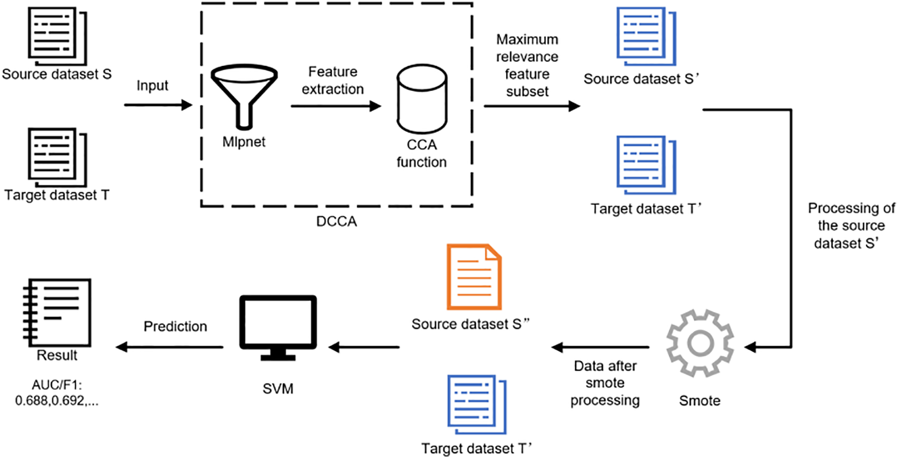
Figure 1: The S-DCCA methodological framework

3.1 Deep Canonical Correlation Analysis Methods

Fig. 2 depicts the schematic diagram of DCCA, which consists of the following steps.

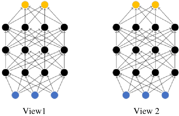
Figure 2: DCCA schematic

The diagram consists of two learning deep networks so that the output layers (the top layers of each network) have maximum correlation. The blue nodes correspond to input features (n1 = n2 = 3), the black nodes are hidden units (c1 = c2 = 4), and the output layer is yellow (o = 2). Both networks have d = 4 layers. Let us assume that each intermediate layer of the first view in the network has c1 units, while the final (output) layer has o units. Let x1∈Rn1 represent the parameters for the first view. The output of the first layer for an instance x1 is given by y1=s(W11x1+b11)∈Rc1, where W11∈Rc1×n1 represents the weight matrix, b11∈Rc1 represents the bias vector, and s:R↦R is a non-linear function applied component-wise. Then, the output y1 can be used to compute the output of the next layer, such as y2=s(W21h1+b21)∈Rc1, and so on, until the final representation f1(x1)=s(Wd1yd−1+bd1)∈Ro is computed for the network with d layers. The instance for the second view, represented by f2(x2), is computed in the same way but with different parameters Wl2 and bl2. The objective is to jointly learn the parameters of both views, Wlυ and blv, to maximize corr(f1(X1),f2(X2)). If α1 represents the vector of all parameters Wl1 and bl1 for the first view for l = 1, ..., d, and α2 represents the vector of all parameters Wl2 and bl2 for the second view, then

(α1∗,α2∗)=argmax(α1,α2)corr(f1(X1;α1),f2(X2;α2))(1)

To obtain (α1∗,α2∗), this paper follows the gradient of the correlation objective estimated based on the training data. Let H1∈Ro×m and H2∈Ro×m be matrices whose columns are the top-layer representations generated by the deep models on the two views, for a training set of size m. Let H¯1=H1−1mH1 be the centered data matrix (or H¯2), and define ∑∧12=1m−1H¯1H¯2' and ∑∧12=1m−1H¯1H¯2' as regularization constants r1 (or Σ^22). Assuming r1 > 0, Σ^11 is positive definite. The parameters Wlυ and blv of DCCA are trained to optimize this quantity using gradient-based optimization. The total correlation of the first k components of H1 and H2 is the sum of the first k singular values of the matrix T=Σ^11−12Σ^12Σ^22−12, when k = o:

corr(H1,H2)=‖ T ‖tr=tr(T′T)12(2)

To compute the gradients of corr(H1,H2) concerning all parameters Wlυ and blv, this paper can compute the gradients concerning H1 and H2 separately and then use back-propagation. If the singular value decomposition of T is given by T=UDV', then

∂corr(H1,H2)∂H1=1m−1(2∇11H¯1+∇12H¯2)(3)

where

∇12=Σ∧11−12UV'Σ∧22−12(4)

∇11=12Σ∧11−12UDU'Σ∧11−12(5)

where ∂corr(H1,H2)∂H2 has a symmetric expression. This method uses a novel non-saturating sigmoid function based on cubic roots to determine the output of nodes in the DCCA network.

3.2 S-DCCA Model Construction

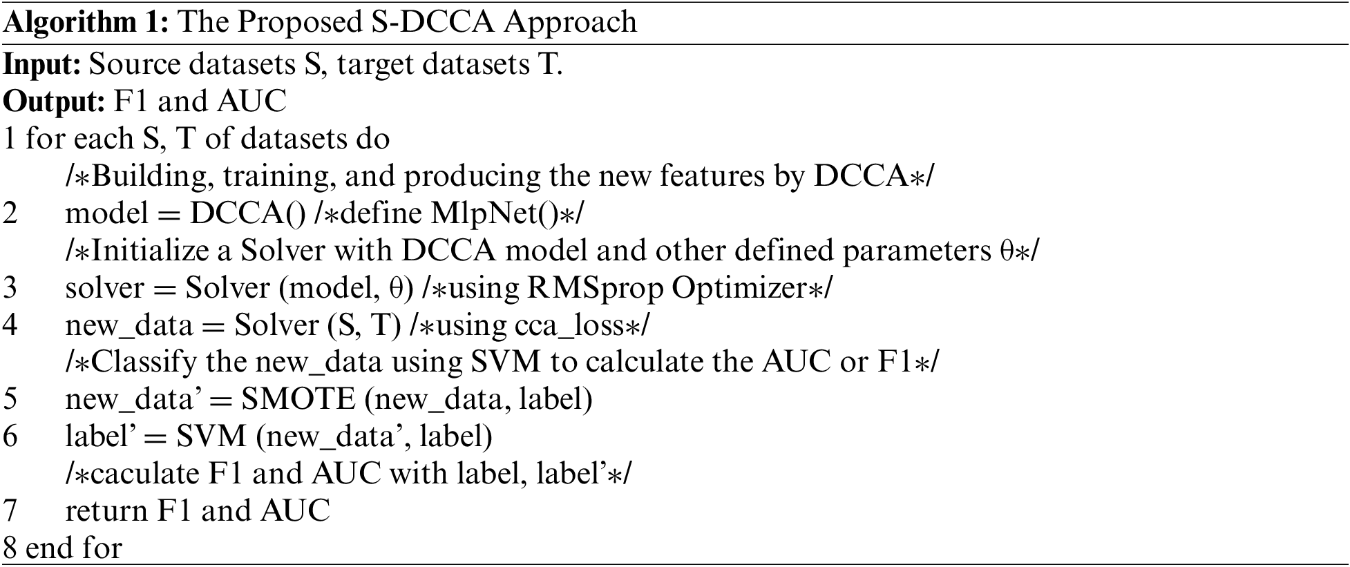
Implementation Steps and Algorithm 1 of the S-DCCA Method:

Loading Data: This paper shows the source dataset and target dataset, converts them into tensors, and preprocesses them. Then, this paper split the data into training and testing sets.

Model Construction: A deep neural network model, MlpNet, is created to map the source dataset and target dataset through nonlinear transformations. The model consists of multiple hidden layers, initialized based on the given number of nodes in each hidden layer and input size. MlpNet is capable of capturing the complex relationships within the dataset and generating more expressive feature representations, thereby providing more accurate and discriminative inputs for subsequent CCA computations.

Defining the Loss Function: This paper uses the CCA loss function to compute the correlation between the two datasets. The computation process includes the following steps:

•   Normalize the outputs of the source dataset and target dataset by subtracting the mean and dividing by the standard deviation;

•   Calculate the covariance matrices of the source dataset and target dataset;

•   Perform singular value decomposition on the covariance matrices to obtain singular values and singular vectors;

•   Compute the correlation based on the singular values and singular vectors.

By optimizing the CCA loss function, the DCCA method maximizes the correlation between the datasets, obtaining the subset of maximally correlated features and improving the joint learning performance of multiple datasets.

Model Training: During the training process, DCCA incorporates the Root Mean Square Propagation (RMSprop) optimizer, which utilizes adaptive learning rates and regularization to optimize the model’s performance. RMSprop is a method used for gradient computation in deep learning, and the regularization term helps prevent overfitting by removing redundant features, resulting in more stable and reliable outcomes. The regularization term typically includes L1 or L2 regularization. L1 regularization helps generate sparse solutions and aids in removing redundant features, while L2 regularization prevents excessive model complexity by preventing the weights from becoming too large. This paper trains the model and optimizes the corresponding parameters such as learning rate, batch size, and regularization parameters.

Model Testing: This paper evaluates the model on the testing set by calculating the loss value and output.

Feature Processing: Based on the division of the training and testing sets, a dataset with new feature data is obtained.

Data Processing: To address the class imbalance, the SMOTE oversampling technique is applied to the preprocessed source dataset, with the corresponding parameters adjusted accordingly.

Classification: This paper employs a linear kernel support vector machine (SVM) to classify the new data. The performance is evaluated using evaluation metrics based on the predictions of the testing set.

In summary, firstly, this paper utilizes a deep neural network to initialize the two input data sets. This paper employs a Multi-Layer Perceptron (MlpNet) to receive the input data and perform non-linear transformations and feature extraction through multiple hidden layers. Each hidden layer consists of a linear layer and an activation function. In the forward propagation process (from the input layer to the output layer), the input data first passes through the linear layer of the first hidden layer. The linear transformation maps the input data to the feature space of the hidden layer. Then, a non-linear transformation is applied to the linearly mapped results through the activation function, introducing a richer representation space. This non-linear transformation and feature extraction process iterates through each hidden layer. Each hidden layer receives the output of the previous hidden layer as input and maps it to a new feature space. Through multiple iterations of hidden layers, the model can gradually learn higher-level abstract feature representations. The last hidden layer does not have an activation function, only a linear layer. This linear layer maps the output of the last hidden layer to the output layer’s dimension. This step can be seen as mapping and reconstructing the extracted features to output the final result. Through this non-linear transformation and feature extraction process, MlpNet can extract more representative and discriminative feature representations from the raw data for subsequent correlation analysis and model training.

Secondly, This paper employs the CCA loss function and selects the top Outdim_size singular values to calculate the correlations using singular value decomposition and eigenvalue decomposition, resulting in the best correlations.

Thirdly, This paper utilizes the RMSprop optimizer to train the extracted feature data, enhancing model performance with adaptive learning rates and regularization. This paper sets the learning rate and regularization term parameters, which facilitate generating sparse solutions to prevent overfitting and achieve the effect of removing redundant features.

Lastly, this paper applies the Smote oversampling technique to the processed data for handling class imbalance. After evaluating the classification results, this paper obtain the detailed steps for constructing the S-DCCA model.

4  Experimental Setup

4.1 Research Questions

To systematically evaluate the proposed S-DCCA method, this paper addresses the following research questions:

RQ1: Which classifier performs the best in the DCCA-based cross-project defect prediction model?

In this study, this paper compares the performance of different classifiers under the same experimental settings to determine which classifier yields the best results. The selected best classifier will be used for subsequent model evaluation.

RQ2: How does the proposed S-DCCA method perform compared to competing CPDP methods?

This paper compares the proposed method with existing state-of-the-art CPDP methods to assess the effectiveness of the predictions obtained after training the S-DCCA model, using evaluation metrics as benchmarks.

RQ3: Does the use of sampling techniques lead to improvement? Which sampling algorithm, when combined with DCCA, yields the best results?

In this study, this paper compares the performance of DCCA combined with other sampling algorithms to assess the effectiveness of DCCA when utilizing sampling methods. By evaluating the metrics, this paper can determine the impact of sampling techniques on the performance of DCCA. Furthermore, this paper identifies the most effective sampling algorithm in combination with DCCA and selects it for subsequent model evaluations.

4.2 Data Set

This paper utilizes four publicly available datasets: ReLink, AEEEM, NASA, and PROMISE [38–40], encompassing a total of 27 projects. Table 1 presents a detailed summary of these repositories. Each project within ReLink, AEEEM, NASA, and PROMISE comprises 26, 61, 21, and 20 metrics, respectively. Bal et al. [41] employed datasets such as AEEEM, NASA, Relink, and PROMISE. Xu et al. [28] utilized datasets including AEEEM, NASA, and Relink. Additionally, Zhao et al. [42] made use of the Relink and AEEEM datasets.

4.3 Evaluation Measures

This paper evaluates the performance of the model using two widely used metrics, namely AUC and F1. These commonly used metrics are adopted in various CPDP approaches. Bal et al. [41] employed the AUC evaluation metric, while Yuan et al. [27] utilized both AUC and F1 metrics. Similarly, Sun et al. [43] employed AUC and F1 metrics. Table 2 presents the confusion matrix, which is a table used to summarize the classification model’s results. True Positive Rate (TPR), also known as recall, refers to the frequency at which the model correctly predicts positive instances out of all actual positive instances. False Positive Rate (FPR) represents the frequency at which the model incorrectly predicts positive instances out of all actual negative instances. The formulas are as follows:

TPR=R=TPTP+FNFPR=FPFP+TN(6)

ROC represents the curve formed by plotting TPR against FPR at different classification thresholds. The area under the ROC curve (AUC) indicates the overall performance of the classification model, with a larger area indicating better performance.

Precision refers to the frequency at which the model correctly predicts positive instances. Recall, on the other hand, is the frequency at which the model correctly identifies positive instances out of all actual positive labels. The formulas are as follows:

Precise=P=TPTP+FPRecall=R=TPTP+FN(7)

The F1 score represents the harmonic mean of precision and recall, providing an overall reflection of the algorithm’s performance. The harmonic mean F1 can reflect the algorithm’s performance as a whole:

F1=2∗P∗RP+R=2TP2TP+FP+FN(8)

Both AUC and F1 score range from 0 to 1, where higher values indicate better predictive performance.

4.4 Comparison Methods

To evaluate the effectiveness of S-DCCA, this paper compares it with a range of representative CPDP methods, including TCA+ [10], CFIW-TNB [13], BurakMHD [14], DMDAJFR [15] and MSCPDP [16]. Nam et al. [10] used the state-of-the-art transfer learning method, TCA, to make the feature distributions in source and target projects similar, and proposed TCA+ which selects appropriate normalization methods for TCA. Zou et al. [13] introduced a CPDP model called CFIW-TNB based on NBC with a dual-weight mechanism, which can improve the performance of predictors better than single-instance weighting or feature weighting. Bhat et al. [14] proposed a training data selection method (BurakMHD) that first transforms the dataset and then filters the training data, which helps select relevant data for CPDP. Zou et al. [15] proposed a novel feature representation learning transfer method that addresses the issue of existing CPDP methods ignoring local representations and mixing instances with different class labels, resulting in problematic fuzzy predictions near the decision boundary. Zhao et al. [16] introduced a new MSCPDP method that can simultaneously utilize knowledge from multiple source projects related to the target project to construct a defect prediction model.

To evaluate whether DCCA benefits from sampling techniques, this paper selected four commonly used sampling techniques, including Random Oversampling (ROS), Random Undersampling (RUS), ADASYN [44], and SMOTE.

4.5 Parameter Settings

Firstly, to address the class imbalance problem, this paper employed the SMOTE [33] sampling technique to alleviate this issue. Secondly, this paper used a linear SVM as the classifier for evaluation, and in Section 5.1, this paper explains why we chose the SVM classifier. For the parameters of the three comparison methods mentioned above, this paper kept them consistent with the original papers. For the size of the new space learned by the S-DCCA model (the number of new features), outdim_size was set to 10. The input sizes for both sets of data, input_shape1, and input_shape2, were set to 61. Regarding the parameters for training the network, this paper utilized the Root Mean Square Propagation (RMSprop) optimizer, with a batch size of 800 samples per training batch. The learning rate was set to 1e-3, and the regularization parameter (reg_par) was set to 1e-5.

4.6 Evaluation Settings

This paper uses 27 projects from four publicly available datasets as the benchmark dataset. To evaluate the performance of the CPDP models, this paper selects one project from the same dataset as the source data and another project as the target data, resulting in 200 combinations. For each combination, this paper randomly samples data from the source dataset and uses 80% of the instances as training data based on the Pareto principle. To assess the performance of CPDP methods, this paper repeats the above steps 30 times and calculates the average performance across all combinations in the same dataset.

4.7 Statistical Test and Effect Size Test

The Scott-Knott ESD test, proposed by Tantithamthavorn et al. [45], is a statistical test method widely used for analyzing whether certain methods are superior to others. It can also generate global rankings for these methods. The Scott-Knott ESD test utilizes hierarchical clustering analysis to divide different methods into significantly distinct groups, where the effect size is not negligible. This ensures that there are no statistically significant performance differences within the same group, while statistically significant performance differences exist between different groups.

5  Experimental Results

5.1 Comparison Results of Classifiers

RQ1: Research Question 1: Which classifier performs the best in the cross-project defect prediction model based on DCCA?

In this study, this article selected 7 projects from the NASA dataset and repeated the steps 10 times.

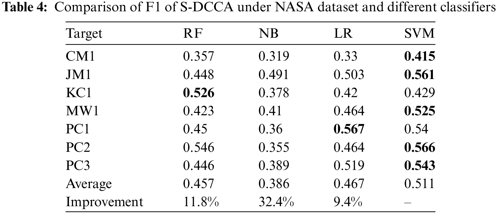
Tables 3 and 4 present the comparison results of AUC and F1 scores for S-DCCA using four different classifiers. The best values are highlighted in bold. From the tables, this article observes that overall, SVM outperforms the other classifiers significantly, achieving the highest AUC of 0.651, which is an improvement of 9.9% to 11.9% compared to the other classifiers. Similarly, it achieves the highest F1 score of 0.566, representing an improvement of 9.4% to 32.4% compared to the other classifiers.

Figs. 3a and 3b depict box plots comparing the performance of different classifiers in terms of AUC and F1 scores, respectively. The top horizontal line represents the maximum value within the non-outlier range, the line within the box represents the median, the cross represents the mean, and the bottom horizontal line represents the minimum value within the non-outlier range. In the figures, higher values for the maximum, median, mean, and minimum indicate better performance in the respective metrics. From the plots, this article can observe that Fig. 3a, on the NASA dataset, the SVM classifier consistently outperforms the other classifiers in terms of the maximum, mean, median, and minimum values. For Fig. 3b, on the NASA dataset, the SVM classifier’s maximum is slightly lower than LR, but the median, mean, and minimum values are superior to the other classifiers.

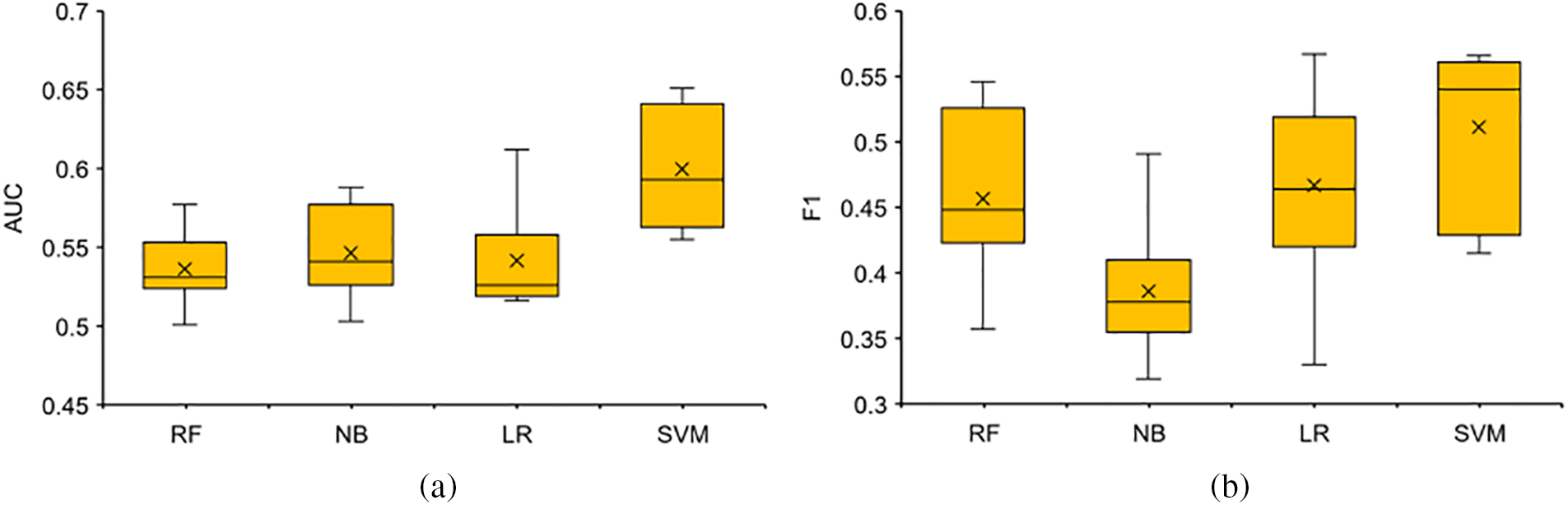
Figure 3: Results of different classifiers indicated by AUC and F1 (box plots)

Figs. 4a and 4b display combined graphs showcasing the performance of different classifiers in terms of AUC and F1 scores, respectively. In the plots, RF, NB, and LR classifiers are represented with bar charts, while the SVM classifier is shown as a line chart. From the figures, this article can observe that in most of the projects within the NASA dataset, the results obtained after applying SVM yield the best results.

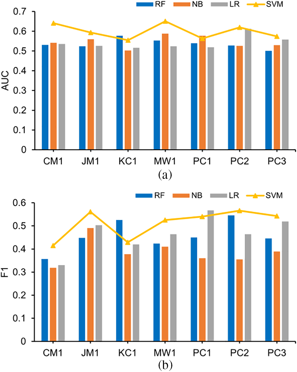
Figure 4: Results of different classifiers indicated by AUC and F1 (combined graph)

Answering RQ1: Based on the results tested on different projects, our SVM classifier outperforms the other classifiers in terms of AUC and F1 values on the NASA dataset. Overall, S-DCCA improves the performance of all classifiers by at least 9.9% and 9.4% in terms of AUC and F1 scores, respectively. Therefore, this article concludes that the SVM classifier exhibits the best performance in terms of evaluation metrics, and thus, this article selects it for training purposes.

5.2 Comparative Results with Baseline

RQ2: How does the proposed S-DCCA method perform compared to competing CPDP methods?

Tables 5 and 6 represent the comparison results of AUC and F1 scores between S-DCCA and other baseline methods. The best values are highlighted in bold. From the tables, this article observes that S-DCCA outperforms more than half of the projects compared to the other baselines, achieving the highest AUC of 0.692, which is an improvement of 1.2% to 10.7% compared to the other baselines. Similarly, it achieves the highest F1 score of 0.601, representing an improvement of 5.5% to 27.6% compared to the other baselines.

Figs. 5a and 5b illustrate box plots comparing the performance of different CPDP methods in terms of AUC and F1 scores, respectively. The top horizontal line represents the maximum value within the non-outlier range, the line within the box represents the median, the cross represents the mean, and the bottom horizontal line represents the minimum value within the non-outlier range. In the figures, higher values for the maximum, median, mean, and minimum indicate better performance in the respective metrics. Here, this article discards outliers. From the plots, this article can observe that Fig. 5a, in comparison with all baseline methods, S-DCCA exhibits the best mean and minimum values despite having a slightly lower median than BurakMHD and a slightly lower maximum than TCA+. However, overall, its performance remains superior. For Fig. 5b, in comparison with all baseline methods, S-DCCA demonstrates the best maximum, mean, and median values (with the median slightly higher than TCA+). Although the minimum value is slightly lower than CFIW-TNB, its overall performance remains the best.

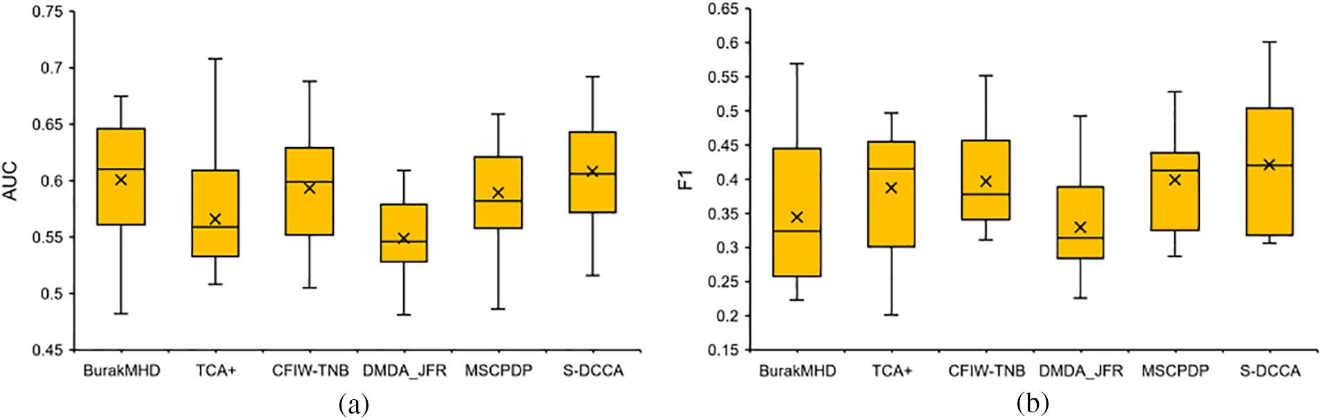
Figure 5: Results of different classifiers indicated by AUC and F1 (box plots)

Figs. 6a and 6b display combined graphs showcasing the performance of different CPDP methods in terms of AUC and F1 scores, respectively. In the plots, the three baseline methods are represented with bar charts, while S-DCCA is shown as a line chart. Due to the large number of projects, only partial project names are displayed on the x-axis. From the figures, this article can observe that in the majority of the projects, the results obtained after applying S-DCCA yield the best performance.

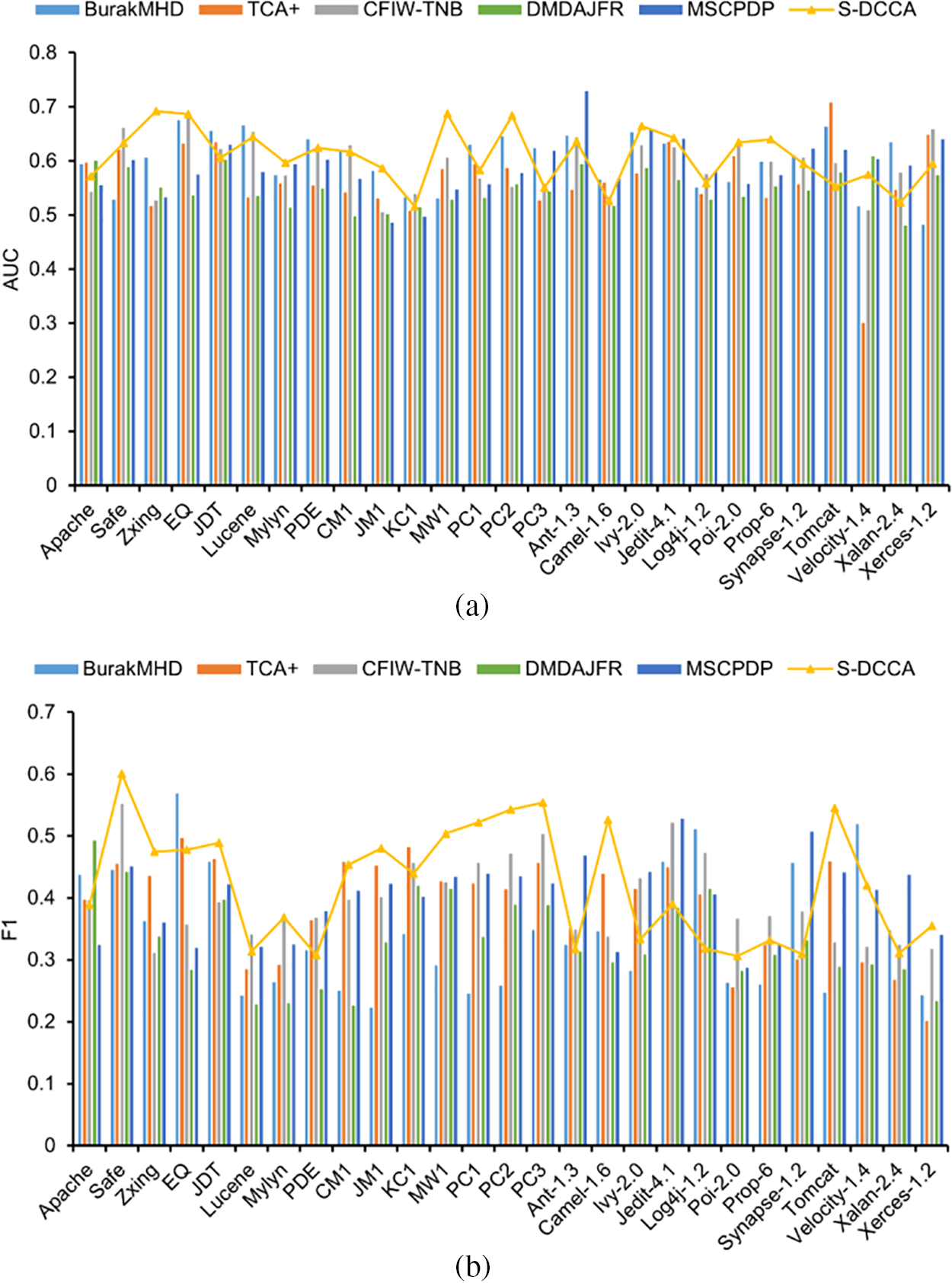
Figure 6: Results of different classifiers indicated by AUC and F1 (combined graph)

Answering RQ2: Based on the results tested on different datasets, our S-DCCA outperforms all baselines in terms of AUC and F1 scores across all datasets. On average, S-DCCA improves the performance of all baselines by at least 1.2% and 5.5% in terms of AUC and F1 scores, respectively.

5.3 Results of Ablation Experiments

RQ3: Does the use of sampling techniques lead to improvement? Which sampling algorithm performs the best when combined with other sampling algorithms?

In this section, this article selected seven projects from the NASA dataset. The experiments were repeated for 10 iterations.

Tables 7 and 8 present the comparison results of AUC and F1 scores for DCCA using four different sampling algorithms, with the best values highlighted in bold. The experiments were conducted with random oversampling (ROS), random undersampling (RUS), ADASYN, and SMOTE. From the tables, this article observed that overall, SMOTE outperformed other sampling techniques, with the highest AUC of 0.688. When combined with DCCA, the performance improved by 1.1% to 6.5%. The highest F1 score was 0.554, with a performance improvement of 0.6% to 7.5% when combined with DCCA and other sampling techniques.

Figs. 7a and 7b present box plots of the AUC and F1 scores for different sampling algorithms. The top horizontal line represents the maximum value within the non-outlier range, the horizontal line within the box represents the median, the cross indicates the mean value, and the bottom horizontal line represents the minimum value within the non-outlier range. In the figures, higher values for the maximum, median, mean, and minimum indicate better performance for the two metrics. This article excluded outliers in the plots. From Fig. 7a, on the NASA dataset, although the median of SMOTE is slightly lower than random undersampling, and the minimum value is lower than ROS and ADASYN, the maximum and mean values are better than other sampling techniques. For Fig. 7b, on the NASA dataset, although the maximum value of SMOTE is lower than ADASYN, the median, mean, and minimum values are better than other sampling techniques.

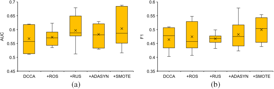
Figure 7: Different sampling techniques results represented by AUC and F1 (box plots)

Figs. 8a and 8b present combined plots of the AUC and F1 scores for different sampling algorithms. ROS, RUS, and ADASYN are represented by bar charts, and SMOTE is represented by a line graph. From the figures, this article can see that in most projects of the NASA dataset, the results obtained after applying SMOTE have the best performance.

Figure 8: Different sampling techniques results represented by AUC and F1 (combined graph)

In response to RQ3: Based on the results tested on different projects, DCCA showed improvement after applying all four sampling techniques. Our SMOTE technique achieved better AUC and F1 averages than other sampling techniques on the NASA dataset. Overall, when combined with all sampling techniques, DCCA’s performance improved by at least 1.2% and 0.6% in terms of AUC and F1, respectively. Therefore, this article concludes that the SMOTE sampling technique can enhance DCCA, and it provides the best improvement. Thus, this article chose to combine DCCA with SMOTE for training.

6  Discussion

6.1 Statistical Test and Effect Size Test Study

Figs. 9a and 9b present the test results of S-DCCA compared to various baseline methods using ScottKnott ESD, represented by AUC and F1 scores. This article utilized box plots to illustrate the results, with the horizontal line in the middle indicating the median. As the median values of the baseline methods have been presented in the previous section, this article will not provide a detailed description of the results in this section. Fig. 9 demonstrates that our S-DCCA method outperforms the state-of-the-art CPDP method. The ScottKnott ESD test further confirms that our S-DCCA method consistently ranks among the top performers in terms of AUC and F1, indicating statistically significant performance differences and non-negligible effect sizes.

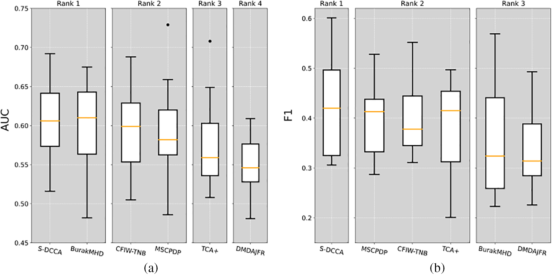
Figure 9: Ranking using ScottKnott ESD represented by AUC and F1

6.2 Implications

The method proposed in this paper is a simple and effective CPDP approach. Previous research has mainly focused on defect prediction within the same project, and many researchers have not considered the issue of non-linear correlations between data in cross-project defect prediction. By introducing the DCCA method, this article proposes S-DCCA, which improves the similarity between the source and target datasets, obtains relevant feature subsets, reduces computational bias in subsequent experiments, and enables accurate defect prediction across different projects. This is also the first application of deep canonical correlation analysis, typically used in image-related fields, to CPDP. The results of this study are valuable for researchers in the field.

6.3 Threats to Validity

This section describes potential threats that may affect our research work in terms of construct, internal, and external aspects.

Regarding construct threats, in real-world classification problems, dataset distributions are often imbalanced. In this study, this article used the SMOTE oversampling technique to alleviate class imbalance issues. However, this algorithm cannot overcome the problem of imbalanced data distribution and may lead to marginalization of the distribution. This article did not consider whether other methods for handling imbalanced data could yield better results, and this article only used AUC and F1 evaluation metrics, which may produce different predictive outcomes when using other evaluation metrics.

Regarding internal threats, it is important to consider factors that may influence experimental results when conducting experiments and comparisons. For methods without available source code, this article used the same parameter settings and carefully implemented them according to the descriptions in the respective papers to mitigate such threats. However, due to potential implementation differences, there may be biases in the comparison between our method and these baseline methods. Additionally, comparisons with other advanced CPDP methods could also be considered. Furthermore, different data partitioning ratios may result in different predictive outcomes. Hence, in our experiments, this article followed the common practice of using the Pareto principle, randomly selecting 80% of the data as training data, and repeating the process 30 times. However, this article did not consider the possibility that selecting different partitioning ratios may yield better results.

Regarding external threats, in this paper, this article utilized four publicly available datasets for experimentation, which are widely applied in various domains [46,47]. Although S-DCCA outperforms current state-of-the-art baseline methods in terms of predictive performance across 27 different projects, there is no guarantee that the same results will be obtained on other datasets. This article did not take into account the possibility of different outcomes on other datasets.

7  Conclusion

This study proposes a cross-project defect prediction method based on SMOTE and deep canonical correlation analysis (S-DCCA) to address the issue of data distribution differences between source and target projects. S-DCCA calculates correlation, selects the subset of highly correlated features, and eliminates redundant features for model training. Finally, based on the comparison results of classifiers, this article selects the support vector machine (SVM) classifier and utilizes the SMOTE oversampling technique to obtain the final prediction results. To evaluate the performance of the S-DCCA method, this article conducts experiments on 27 projects from four publicly available datasets and uses AUC and F1 scores as evaluation metrics. The experimental results demonstrate that S-DCCA outperforms other baseline methods in terms of prediction effectiveness and exhibits good performance. This indicates that the S-DCCA method can accurately predict defects across different projects. With its simplicity and effectiveness, S-DCCA can assist researchers in reliable defect prediction among diverse projects. S-DCCA represents a feasible novel CPDP method that reduces data distribution differences between source and target projects, thereby improving the performance of cross-project defect prediction.

For future work, this article will investigate transfer learning methods to address class imbalance issues and incorporate them into the S-DCCA method to further enhance the predictive performance of CPDP. Transfer learning excels at transferring knowledge across domains, which aligns with the main idea of addressing data distribution differences in CPDP. Despite having the same set of metrics, the inherent differences between source and target projects manifest in the diversity of data distribution. Therefore, our focus will be on how to combine transfer learning to mitigate marginal distribution differences and conditional distribution differences between source and target projects. Several methods have been proposed to reduce marginal and conditional distribution disparities. Long et al. [48] introduced Joint Distribution Adaptation (JDA) to minimize the distance between the joint probability distributions of the source and target domains. However, JDA falls short in addressing the discrepancy between marginal and conditional distribution adaptations, with varying degrees of importance. Wang et al. [49] proposed Balanced Distribution Adaptation (BDA), which incorporates a balancing factor, denoted as μ, to adaptively adjust the importance of marginal and conditional distribution alignment based on specific data domains. Nevertheless, BDA does not address the precise calculation issue of the balancing factor μ. To tackle this, Wang et al. [50] presented Dynamic Distribution Adaptation (DDA), which treats μ as a parameter in the migration process and determines its optimal value through cross-validation. By integrating the DDA transfer learning method, this article can better adjust the marginal and conditional distributions to address class imbalance issues.

Acknowledgement: The authors would like to thank the Software Testing and Evaluation Center, Nanchang Hangkong University for providing facilities to conduct the research.

Funding Statement: National Natural Science Foundation of China, Grant/Award Number: 61867004; National Natural Science Foundation of China Youth Fund, Grant/Award Number: 41801288.

Author Contributions: The authors confirm contribution to the paper as follows: Study conception and design: S. Zhang; data collection: S. Zhang, K. Wu; analysis and interpretation of results: S. Zhang, X. Fan, K. Wu; draft manuscript preparation: S. Zhang, X. Fan; fund support: Y. Ge; provision of laboratory equipment: W. Zheng. All authors reviewed the results and approved the final version of the manuscript.

Availability of Data and Materials: The dataset of this paper can be obtained from the following link: https://github.com/ZSQ1025/S-DCCA.

Conflicts of Interest: The authors declare that they have no conflicts of interest to report regarding the present study.

References

1. R. Yedida and T. Menzies, “On the value of oversampling for deep learning in software defect prediction,” IEEE Transactions on Software Engineering, vol. 48, no. 8, pp. 3103–3116, 2021. [Google Scholar]

2. T. Menzies, J. D. Stefano, A. B. Bener and B. Turhan, “On the relative value of cross-company and within-company data for defect prediction,” Empirical Software Engineering, vol. 14, no. 5, pp. 540–578, 2009. [Google Scholar]

3. J. Nam, W. Fu, S. Kim, T. Menzies and L. Tan, “Heterogeneous defect prediction,” IEEE Transactions on Software Engineering, vol. 44, no. 9, pp. 874–896, 2018. [Google Scholar]

4. Z. Thomas, G. Harald, M. Brendan, G. Emanuel and N. Nachiappan, “Cross-project defect prediction: A large scale experiment on data vs. domain vs. process,” in Proc. of ESEC/FSE, New York, NY, USA, pp. 91–100, 2009. [Google Scholar]

5. J. W. Keung, K. Matsumoto, H. Hata, K. Bennin and N. Limsettho, “Cross project defect prediction using class distribution estimation and oversampling,” Information and Software Technology, vol. 100, pp. 87–102, 2018. https://doi.org/10.1016/j.infsof.2018.04.001 [Google Scholar] [CrossRef]

6. S. Wang, T. Y. Liu, J. Nam and L. Tan, “Deep semantic feature learning for software defect prediction,” IEEE Transactions on Software Engineering, vol. 46, no. 12, pp. 1267–1293, 2018. [Google Scholar]

7. C. Ni, X. Xia, D. Lo, X. Chen and Q. Gu, “Revisiting supervised and unsupervised methods for effort-aware cross-project defect prediction,” IEEE Transactions on Software Engineering, vol. 46, no. 12, pp. 1267–1293, 2018. [Google Scholar]

8. X. Y. Jing, F. Wu, B. W. Xu and X. W. Dong, “An improved SDA based defect prediction framework for both within-project and cross-project class-imbalance problems,” IEEE Transactions on Software Engineering, vol. 43, no. 4, pp. 321–339, 2016. [Google Scholar]

9. L. L. Bo, L. Jiang, J. Y. Qian, S. J. Jiang and L. N. Gong, “A novel class-imbalance learning approach for both within-project and cross-project defect prediction,” IEEE Transactions on Reliability, vol. 69, no. 1, pp. 40–54, 2019. [Google Scholar]

10. J. Nam, S. J. Pan and S. Kim, “Transfer defect learning,” in 2013 IEEE Conf. on Int. Conf. on Software Engineering, San Francisco, CA, USA, pp. 18–26, 2013. [Google Scholar]

11. D. Ryu, O. Choi and J. Baik, “Value-cognitive boosting with a support vector machine for cross-project defect prediction,” Empirical Software Engineering, vol. 21, pp. 43–71, 2016. https://doi.org/10.1007/s10664-014-9346-4 [Google Scholar] [CrossRef]

12. X. Jing, F. Wu, X. Dong, F. Qi and B. Xu, “Heterogeneous cross-company defect prediction by unified metric representation and CCA-based transfer learning,” in Proc. of ESEC/FSE, Bergamo Italy, pp. 496–507, 2015. [Google Scholar]

13. Q. Zou, L. Lu, S. Qiu, Z. Y. Cai and X. W. Gu, “Correlation feature and instance weights transfer learning for cross project software defect prediction,” IET Software, vol. 15, no. 1, pp. 55–74, 2021. [Google Scholar]

14. N. A. Bhat and S. U. Farooq, “An improved method for training data selection for cross-project defect prediction,” Arabian Journal for Science and Engineering, vol. 47, no. 2, pp. 1939–1954, 2022. [Google Scholar]

15. Q. Zou, L. Lu, Z. Yang, X. Gu and S. Qiu, “Joint feature representation learning and progressive distribution matching for cross-project defect prediction,” Information and Software Technology, vol. 137, no. 2, pp. 1939–1954, 2021. [Google Scholar]

16. Y. Zhao, Y. Zhu, Q. Yu and X. Chen, “Cross-project defect prediction considering multiple data distribution simultaneously,” Symmetry, vol. 14, no. 2, pp. 401, 2022. https://doi.org/10.3390/sym14020401 [Google Scholar] [CrossRef]

17. W. Wen, B. Zhang, X. Gu and X. Ju, “An empirical study on combining source selection and transfer learning for cross-project defect prediction,” in 2019 IEEE Conf. on Intelligent Bug Fixing (IBF), Hangzhou, China, pp. 29–38, 2019. [Google Scholar]

18. C. Liu, D. Yang, X. Xia, M. Yan and X. H. Zhang, “A two-phase transfer learning model for cross-project defect prediction,” Information and Software Technology, vol. 107, pp. 125–136, 2019. https://doi.org/10.1016/j.infsof.2018.11.005 [Google Scholar] [CrossRef]

19. T. Asano, M. Tsunoda, K. Toda, A. Tahir, K. Nakasai et al., “Using bandit algorithms for project selection in cross-project defect prediction,” in 2021 IEEE Conf. on Software Maintenance and Evolution, Luxembourg, pp. 649–653, 2021. [Google Scholar]

20. S. Qiu, L. Lu and S. Jiang, “Joint distribution matching model for distribution-adaptation-based cross-project defect prediction,” IET Software, vol. 13, no. 5, pp. 393–402, 2019. [Google Scholar]

21. K. Li, Z. Xiang, T. Chen, S. Wang and K. C. Tan, “Understanding the automated parameter optimization on transfer learning for cross-project defect prediction: An empirical study,” in Proc. ACM/IEEE, New York, NY, USA, pp. 566–577, 2020. [Google Scholar]

22. R. Vashisht and S. A. M. Rizvi, “Feature extraction to heterogeneous cross project defect prediction,” in Proc. of ICRITO, Noida, India, pp. 1221–1225, 2020. [Google Scholar]

23. C. Cui, B. Liu and S. Wang, “Isolation forest filter to simplify training data for cross-project defect prediction,” in Proc. of PHM-Qingdao, Qingdao, China, pp. 1–6, 2019. [Google Scholar]

24. Q. Yu, J. Qian, S. Jiang, Z. Wu and G. Zhang, “An empirical study on the effectiveness of feature selection for cross-project defect prediction,” IEEE Access, vol. 7, pp. 35710– 35718, 2019. https://doi.org/10.1109/ACCESS.2019.2895614 [Google Scholar] [CrossRef]

25. F. Peters, T. Menzies and A. Marcus, “Better cross company defect prediction,” in Proc. of MSR, San Francisco, CA, USA, pp. 409–418, 2013. [Google Scholar]

26. P. He, Y. He, L. Yu and B. Li, “An improved method for cross-project defect prediction by simplifying training data,” Mathematical Problems in Engineering, vol. 2018, 2018. https://doi.org/10.1155/2018/2650415 [Google Scholar] [CrossRef]

27. Z. Yuan, X. Chen, Z. Cui and Y. Mu, “ALTRA: Cross-project software defect prediction via active learning and tradaboost,” IEEE Access, vol. 8, pp. 30037–30049, 2020. https://doi.org/10.1109/ACCESS.2020.2972644 [Google Scholar] [CrossRef]

28. Z. Xu, S. Pang, T. Zhang, X. P. Luo, J. Liu et al., “Cross project defect prediction via balanced distribution adaptation based transfer learning,” Journal of Computer Science and Technology, vol. 34, no. 5, pp. 1039–1062, 2019. [Google Scholar]

29. G. Andrew, R. Arora, J. Bilmes and K. Livescu, “Deep canonical correlation analysis,” in Proc. of ICML, Atlanta, GA, USA, pp. 1247–1255, 2013. [Google Scholar]

30. H. Hotelling, “Relations between two sets of variates,” Breakthroughs in Statistics: Methodology and Distribution, vol. 28, pp. 162–190, 1992. https://doi.org/10.1093/biomet/28.3-4.321 [Google Scholar] [CrossRef]

31. Z. Li, X. Y. Jing, F. Wu, X. Zhu, B. Xu et al., “Cost-sensitive transfer kernel canonical correlation analysis for heterogeneous defect prediction,” Automated Software Engineering, vol. 25, no. 2, pp. 201–245, 2018. [Google Scholar]

32. W. Liu, J. L. Qiu, W. L. Zheng and B. L. Lu, “Multimodal emotion recognition using deep canonical correlation analysis,” arXiv:1908.05349, 2019. [Google Scholar]

33. N. V. Chawla, K. W. Bowyer, L. O. Hall and W. P. Kegelmeyer, “SMOTE: Synthetic minority over-sampling technique,” Journal of Artificial Intelligence Research, vol. 16, pp. 321–357, 2002. [Google Scholar]

34. L. Goel, M. Sharma, S. K. Khatri, D. Damodaran and M. Sharma, “Cross-project defect prediction using data sampling for class imbalance learning: An empirical study,” International Journal of Parallel, Emergent and Distributed Systems, vol. 36, no. 2, pp. 130–143, 2021. [Google Scholar]

35. K. Cheng, C. Zhang, H. Yu, X. Yang, H. Zou et al., “Grouped SMOTE with noise filtering mechanism for classifying imbalanced data,” IEEE Access, vol. 7, pp. 170668–170681, 2019. https://doi.org/10.1109/ACCESS.2019.2955086 [Google Scholar] [CrossRef]

36. K. E. Bennin, J. W. Keung and A. Monden, “On the relative value of data resampling approaches for software defect prediction,” Empirical Software Engineering, vol. 24, pp. 602–636, 2019. https://doi.org/10.1007/s10664-018-9633-6 [Google Scholar] [CrossRef]

37. S. Gao, W. Dong, K. Cheng, X. Yang, S. Zheng et al., “Adaptive decision threshold-based extreme learning machine for classifying imbalanced multi-label data,” Neural Processing Letters, vol. 52, no. 3, pp. 2151–2173, 2020. [Google Scholar]

38. B. Caglayan, E. Kocaguneli, J. Krall, F. Peters and B. Turhan, “The PROMISE repository of empirical software engineering data,” West Virginia University Department of Computer Science, 2012. US1665662A [Google Scholar]

39. M. D. Ambros, M. Lanza and R. Robbes, “Evaluating defect prediction approaches: A benchmark and an extensive comparison,” Empirical Software Engineering, vol. 17, no. 4–5, pp. 531–577, 2012. [Google Scholar]

40. R. Wu, H. Zhang, S. Kim and S. C. Cheung, “Relink: Recovering links between bugs and changes,” in Proc. of ESEC/FSE, New York, NY, USA, pp. 15–25, 2011. [Google Scholar]

41. P. R. Bal and S. Kumar, “A data transfer and relevant metrics matching based approach for heterogeneous defect prediction,” IEEE Transactions on Software Engineering, vol. 49, no. 3, pp. 1232–1245, 2022. [Google Scholar]

42. Y. Zhao, Y. Zhu, Q. Yu and X. Chen, “Cross-project defect prediction method based on manifold feature transformation,” Future Internet, vol. 13, no. 8, pp. 216, 2021. [Google Scholar]

43. Z. Sun, J. Li, H. Sun and L. He, “CFPS: Collaborative filtering based source projects selection for cross-project defect prediction,” Applied Soft Computing, vol. 99, pp. 216, 2021. https://doi.org/10.1016/j.asoc.2020.106940 [Google Scholar] [CrossRef]

44. H. He, Y. Bai, E. A. Garcia and S. Li, “ADASYN: Adaptive synthetic sampling approach for imbalanced learning,” in Proc. of IJCNN, Hong Kong, China, pp. 1322–1328, 2008. [Google Scholar]

45. C. Tantithamthavorn, S. McIntosh, A. E. Hassan and K. Matsumoto, “An empirical comparison of model validation techniques for defect prediction models,” IEEE Transactions on Software Engineering, vol. 43, no. 1, pp. 1–18, 2016. [Google Scholar]

46. Z. Li, X. Y. Jing, X. Zhu, H. Zhang, B. Xu et al., “On the multiple sources and privacy preservation issues for heterogeneous defect prediction,” IEEE Transactions on Software Engineering, vol. 45, no. 4, pp. 391–411, 2019. [Google Scholar]

47. Y. Zhou, Y. Yang, H. Lu, L. Chen, Y. Li et al., “How far we have progressed in the journey? An examination of cross-project defect prediction,” ACM Transactions on Software Engineering and Methodology, vol. 27, no. 1, pp. 1–51, 2018. [Google Scholar]

48. M. Long, J. Wang, G. Ding, J. Sun and P. S. Yu, “Transfer feature learning with joint distribution adaptation,” in Proc. of ICCV, Sydney, Australia, pp. 2200–2207, 2013. [Google Scholar]

49. J. Wang, Y. Chen, S. Hao, W. Feng and Z. Shen, “Balanced distribution adaptation for transfer learning,” in Proc. of ICDM, New Orleans, LA, USA, pp. 1129–1134, 2017. [Google Scholar]

50. J. Wang, Y. Chen, H. Yu, W. Feng, M. Huang et al., “Transfer learning with dynamic distribution adaptation,” ACM Transactions on Intelligent Systems and Technology, vol. 11, no. 1, pp. 1–25, 2020. [Google Scholar]