A Security Trade-Off Scheme of Anomaly Detection System in IoT to Defend against Data-Tampering Attacks

1  Introduction

Internet of Things (IoT) as a bridge connecting the physical world with the digital world has extensive applications in modern society [1,2] Due to the constrained computational power and memory capacity of IoT devices, along with the limited bandwidth of wireless communications, IoT are susceptible to a broad spectrum of cyber attacks [3–5]. In particular, the real data in IoT can be tampered with through session hijacking [6] or physical capture [7], which may lead to serious consequences [8–10]. Consequently, protecting IoT from data-tampering (DT) attacks is a major issue in the domain of IoT security [11,12].

1.1 Anomaly Detection System

To protect IoT from DT attacks, defense techniques based on signature [13,14] or anomaly [15–17] have been developed. Deploying anomaly detection systems (ADSs) in some or all nodes of IoT proves to be an effective means of defending against DT attacks. Real-world IoT may contain many resource-constrained devices that can only use lightweight ADSs to defend against DT attacks. When confronted with sophisticated data tampering attacks, some of these lightweight ADSs may exhibit high false positive rate. An ADS can be configured to operate in either active or passive mode. In the active mode, a portion of authentic data may be discarded due to the false positive reports of an ADS. On the other hand, in the passive mode, all false data will go unregulated and bring various security issues to IoT. In practice, both discarding authentic data and accepting false data have negative impact. Therefore, it is crucial to devise a strategy for managing the anomaly detection system to minimize the impact of false data, while also accepting a low probability of discarding genuine data [18–20].

In this paper, we focus our attention on IoT of two types of nodes: sensing nodes used for collecting the environmental data, and cluster heads used for forwarding the data coming from sensing nodes to the data center. All the cluster heads are equipped with ADS and work in this way: First, conduct a clustering operation on a set of data coming from different sensing nodes but with the same time stamp. Second, identify all the outlier data as abnormal and discard them. Finally, encode all the remaining data and deliver the encrypted data to the data center [21,22].

Currently, machine learning-based anomaly detection techniques are widely applied to IoT [23–25]. These techniques can identify abnormal and malicious behavior by analyzing and learning from normal network traffic and behavior patterns. For instance, employing machine learning algorithms to analyze IoT data can help establish normal data patterns, triggering an alert in the event of any anomalies. By applying machine learning-based anomaly detection techniques, cluster head nodes can promptly detect potential intrusion behavior and take appropriate security measures to protect the overall security of the IoT system. However, it is important to note that while this technique can help identify potential malicious threats, it also has limitations and challenges. For instance, a significant amount of labeled data is required for training in the machine learning process, which can be difficult to obtain and label for real-time data in the IoT. Additionally, some machine learning algorithms are not lightweight and may not be suitable for resource-constrained Io.

Although the operation of ADSs can enhance the security of IoT, the presence of high false positive rates in some ADSs may result in authentic data being incorrectly identified as false data, rendering it inaccessible and potentially disrupting the normal functioning of the IoT. This issue, known as the security trade-off (ST) problem, presents a trade-off between the security and availability of data in IoT. Therefore, it is crucial to find an effective ADS management scheme that maximizes security performance without disrupting the normal operation of IoT. This paper aims to deal with the problem.

1.2 Main Contributions

The main contributions of this paper are sketched as follows:

•   The ST problem is modeled as a linear programming we refer to as the ST model, where the objective function denotes the combined detection rate of the ADS bank in a running mode, the constraint reflects the demand for a low combined false alarm rate of the ADS bank, and an optimal solution stands for a running mode of the ADS bank that maximizes the combined detection rate subject to a low combined false alarm rate.

•   The ST model is solved analytically, respectively, accompanied with a few numeric examples. The effect of some factors on the maximum combined detection rate is revealed through theoretical analysis. Simulations show that the ADS management scheme can mitigate the data unavailability loss caused by the high false positive rates in ADSs.

To our knowledge, this is the first time the issue of protecting IoT from DT attacks is addressed from a holistic perspective. The subsequent materials are organized in this fashion: Section 2 reviews the related work. Section 3 reduces the ST problem to the ST model, Section 4 solves the ST model analytically, and Section 5 solves the ST model using a network simulator. Section 6 reveals the effect of some factors on the maximum combined detection rate. This work is summarized in Section 7.

2  Related Work

In the past decade, a multitude of anomaly-based detection techniques for IoT have been developed. These detection techniques can be broadly classified into two categories: local agent-based detection techniques, and global agent-based detection techniques. Below let us briefly review the two types of detection techniques.

2.1 Local Agent-Based Detection Techniques

It is meant by local agent-based detection that ADSs are deployed in all nodes of an IoT, and different ADSs cooperate to achieve a good detection performance [26]. This type of detection technique comes at the cost of increased communication overhead.

Reference [27] proposes a localized algorithm for detecting insider attackers in IoT. Reference [28] introduces a distributed ADS employing fog computing to identify DDoS attacks in IoT. Reference [29] advises a host-based false data injection detection method for smart grid cyber-physical systems. All these detection techniques require each node to broadcast its newest readings to its neighborhood in a real-time manner, tremendously increasing the communication overhead.

Reference [30] develops a game theory-based, incentive-driven detection mechanism for IoT. This mechanism can be used to protect free-riding attacks. Reference [31] suggests a game theory-based collaborative security detection approach for IoT. These mechanisms require frequent information exchange between different nodes, significantly increasing the communication overhead. Reference [32] proposes an efficient ADS deployment architecture for multi-hop clustered wireless sensor networks, and a resource allocation strategy was developed in this paper to improve the performance of the ADS.

2.2 Global Agent-Based Detection Techniques

When it comes to global agent-based detection, ADSs are only deployed in cluster heads of an IoT [33–35]. As compared with local agent-based detection techniques, the communication overhead for this type of detection technique is alleviated significantly, at the expense of increased computation overhead of cluster heads. Since the communication cost of an IoT is several orders of magnitude higher than its computation cost, trading the latter for the former is favorable [36].

Reference [34] introduces a hierarchical framework for intrusion detection in industrial IoT. Reference [37] suggests a detection mechanism for cluster-based IoT. Reference [38] presents a distributed, cluster-based anomaly detection algorithm. Reference [39] proposes a fully distributed general-anomaly-detection (GAD) scheme for networked industrial sensing systems. Reference [40] proposes a signaling game-based intrusion detection mechanism to identify malicious vehicle nodes in Vehicular Ad-Hoc Networks (VANETs).

The management of ADS has recently received considerable interest. Reference [15] proposes a Bayesian game approach for intrusion detection in Ad Hoc networks, reference [16] models the security detection in cyber-physical embedded systems as a static game, and reference [17] develops a game theoretical analysis framework for collaborative security detection in IoT systems. All of these studies focus on designing a management and control scheme for individual IoT devices.

2.3 A Comparison with Our Work

Drawing inspiration from established detection techniques for IoT, this paper introduces a management scheme for the anomaly detection system (ADS) in a two-hop IoT network, utilizing a global agent-based detection approach. Unlike the methodologies outlined in references [13,14], which primarily focus on defending against DT attacks using signature-based methods, this study introduces an anomaly-based approach. Furthermore, our study diverges from [18–20] in that we endeavor to propose an Anomaly Detection System (ADS) management scheme for the entire IoT system, whereas their research centered on devising a management scheme for individual IoT devices. Our approach guarantees the global optimality of the running mode for ADSs in an IoT. In contrast, their work may lead to a locally optimal running mode when applied to two-hop IoT.

3  The Modeling of the ST Problem

This section is devoted to the modeling of the ST problem. First, we introduce basic terms and notations. Second, we estimate the combined detection rate of the ADS bank in a running mode. Next, we measure the combined false alarm rate of the ADS bank in a running mode. Finally, we finish the modeling work.

3.1 Data Transmission and Anomaly Detection

Consider a two-hop IoT as was mentioned in Subsection 1.2. Let U={u1,u2,⋯,uN} denote the set of cluster heads of the IoT. Let V(u) denote the set of sensing nodes that are routed to the cluster head u. Then u is the set of sensing nodes of the IoT. Let 𝒱={V(u):u∈U}. The topological structure of the IoT can be characterized by the ordered pair (U,𝒱).

Example 1. Fig. 1 displays the topological structure (U,𝒱) of a two-hop IoT. Here, U={u1,u2,u3}, V(u1)={v1,v2}, V(u2)={v3,v4,v5}, V(u3)={v6,v7,v8,v9,v10}, 𝒱={V(u1),V(u2),V(u3)}.

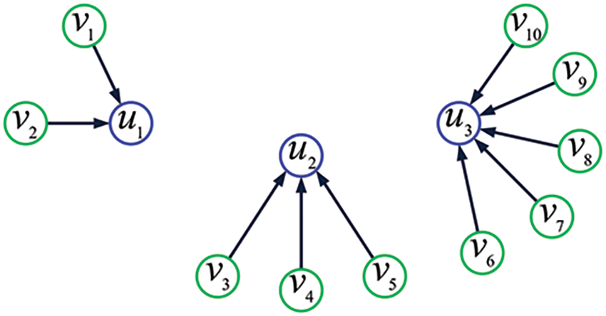
Figure 1: The topology of a two-hop IoT. Here, each green circle denotes a sensing node, each blue circle denotes a cluster head, and each arrow

Let qTP denote the detection rate (equivalently, true positive rate) of the ADS deployed in all cluster heads of the IoT. This implies the ADS identifies false data as abnormal (resp. normal) with probability qTP (resp. 1−qTP). Let qFP denote the false alarm rate (equivalently, false positive rate) of the ADS. This implies the ADS identifies real data as abnormal (resp. normal) with probability qFP (resp. 1−qFP).

Let rv (bits per second) denote the predetermined data-collecting rate of the sensing node v. Then the cluster head u receives data at a rate of ∑v∈V(u)rv bits per second. Let ℛ denote the multiset of the data-collecting rates of sensing nodes of the IoT, i.e., ℛ={rv:v∈V}. We refer to ℛ as a data-collecting scheme assigned to the IoT.

In view of the function of the IoT, we assume rv>0 for all v∈V.

Example 2. Fig. 2 exhibits a data-collecting scheme assigned to the IoT topology shown in Fig. 1.

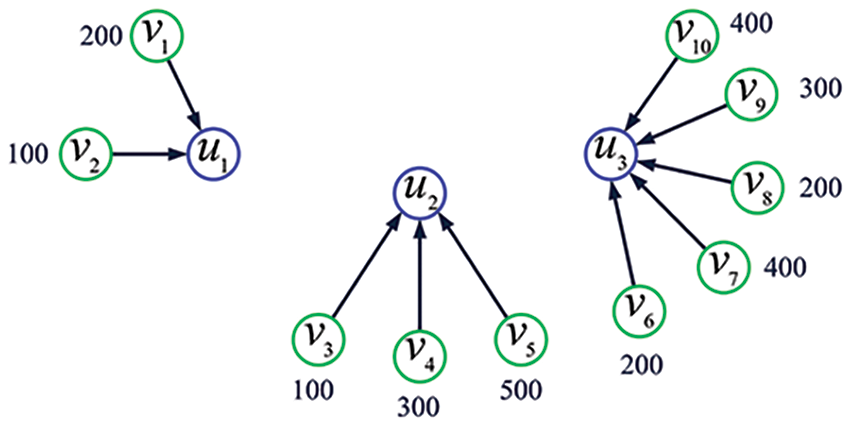
Figure 2: A data-collecting scheme assigned to the IoT topology shown in Fig. 1. Here, the number next to each green circle denotes the data-collecting rate of the corresponding sensing node (unit: bit per second)

Suppose the IoT is subjected to DT attack. Let pv denote the probability with which the real data stored within the sensing node v are replaced with false data. Then the cluster head u receives real data (resp. false data) at an average rate of ∑v∈V(u)(1−pv)rv (resp. ∑v∈V(u)pvrv) bits per second, respectively. Let 𝒫 denote the multiset of the data-tampering probabilities associated with sensing nodes of the IoT, i.e., 𝒫={pv:v∈V}. We refer to 𝒫 as a data-tampering (DT) pattern.

Since the real data are vulnerable to data-tampering attack, we assume pv>0 for all v∈V. On the other hand, to avoid anomaly detection, the attacker would only tamper with a fraction of the real data. Therefore, we assume pv<1 for all v∈V. An ADS is effective if it has a large detection rate and a small false alarm rate, i.e., it identifies most false data (resp. most real data) as abnormal (resp. normal). Hence, it is appropriate to estimate pv (v∈V) as the frequency of the data delivered by v being identified as abnormal.

Example 3. Fig. 3 exhibits a DT pattern on the IoT topology shown in Fig. 1.

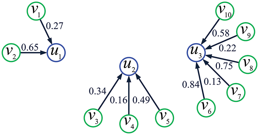
Figure 3: A DT pattern on the IoT topology shown in Fig. 1. Here, the number next to each arrowed line denotes the data-tampering probability for the corresponding sensing node

Combining the above discussions, we get that the IoT can be characterized by the 6-tuple (U,𝒱,qTP,qFP,ℛ,𝒫).

Example 4. By combining Examples 1–3 and assuming qTP=0.9, qFP=0.15, we get the IoT displayed in Fig. 4.

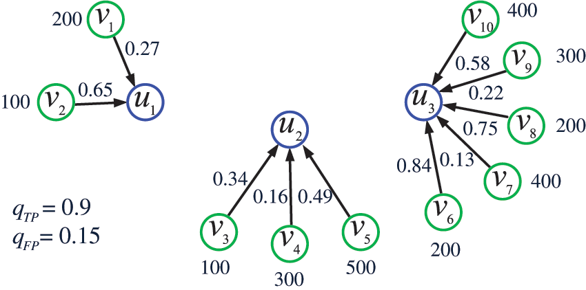
Figure 4: The IoT obtained by combining Examples 1–3 and assuming qTP=0.9, qFP=0.15

At the end of this subsection, let xi denote the running probability of the ADS deployed in the cluster head ui. We refer to the vector

x=(x1,x2,⋯,xN)(1)

as a running mode of the ADS bank.

3.2 Combined Detection Rate

It follows from the notations introduced in the previous subsection that the cluster head ui receives false data at an average rate of ∑v∈V(ui)pvrv bits per second, and identifies the received false data as abnormal at an average rate of qTPxi∑v∈V(ui)pvrv bits per second. So, the set of cluster heads as a whole receives false data at an average rate of ∑i=1N∑v∈V(ui)pvrv bits per second, and identifies the received false data as abnormal at an average rate of ∑i=1NqTPxi∑v∈V(ui)pvrv bits per second. Hence, the average fraction of the false data that are identified as abnormal in all false data is

D(x)=∑i=1NqTPxi∑v∈V(ui)pvrv∑i=1N∑v∈V(ui)pvrv.(2)

We refer to the quantity as the combined detection rate of the ADS bank in the running mode x.

Let

ai=qTP∑v∈V(ui)pvrv∑j=1N∑v∈V(uj)pvrv,1≤i≤N.(3)

It follows from rv>0 and 1 > pv>0 that ai>0, 1≤i≤N. Let a=(a1,a2,⋯,aN). Then

D(x)=∑i=1Naixi=axT.(4)

Hereafter, the superscript T stands for transpose.

3.3 Combined False Alarm Rate

It follows from the notations introduced in Subsection 3.1 that the cluster head ui receives real data at an average rate of ∑v∈V(ui)(1−pv)rv bits per second, and identifies the received real data as abnormal at an average rate of qFPxi∑v∈V(ui)(1−pv)rv bits per second. So, the set of cluster heads as a whole receives real data at an average rate of ∑i=1N∑v∈V(ui)(1−pv)rv bits per second, and identifies the received real data as abnormal at an average rate of ∑i=1NqFPxi∑v∈V(ui)(1−pv)rv bits per second. Hence, the average fraction of the real data that are identified as abnormal in all real data is

A(x)=∑i=1NqFPxi∑v∈V(ui)(1−pv)rv∑i=1N∑v∈V(ui)(1−pv)rv.(5)

We refer to the quantity as the combined false alarm rate of the ADS bank in the running mode x.

Let

bi=qFP∑v∈V(ui)(1−pv)rv∑j=1N∑v∈V(uj)(1−pv)rv,1≤i≤N.(6)

It follows from rv>0 and 1 > pv>0 that bi>0, 1≤i≤N. Let b=(b1,b2,⋯,bN). Then

A(x)=∑i=1Nbixi=bxT.(7)

3.4 The Linear Programming Modeling

We are ready to finish the modeling work. Let θ be the imposed upper bound on the combined false alarm rate, i.e., A(x)≤θ. Based on the discussions in the previous two subsections, the ST problem boils down to the following linear programming:

maxD(x)=∑i=1Naixis.t.{∑i=1Nbixi≤θ,0≤xi≤1,1≤i≤N.(8)

We refer to this linear program as the running mode (RM) model. This model can be abbreviated as

maxD(x)=axTsubject to bxT≤θ,x∈[0,1]N.(9)

Additionally, this model can be characterized by the 7-tuple ℒ𝒫=(U,𝒱,qTP,qFP,ℛ,𝒫,θ).

According to linear programming theory, it can be inferred that the ST model is solvable in polynomial time [38]. In practical applications, the ST model can be efficiently solved by leveraging the optimization toolbox of MATLAB [39].

4  A Theoretical Study of the ST Model

In the preceding section, we introduced a mathematical model, referred to as the ST model. In this section, we embark on a theoretical exploration of the ST model. Initially, we resolve the ST model through analytical approach. Subsequently, we address a submodel derived from the ST model.

4.1 Basic Theorems

The following two theorems together offer a complete solution of the ST model:

Theorem 1. The linear program (8) with θ≥qFP admits x∗=(1,⋯,1) as the unique optimal solution.

Proof: For each x∈[0,1]N, we have A(x)=∑i=1Nbixi≤∑i=1Nbi=qFP≤θ. So, [0,1]N is the feasible set of the linear program. For each x∈[0,1]N, we have D(x)=∑i=1Naixi≤∑i=1Nai=D(x∗). Hence, x∗ is an optimal solution to the linear program. Since the equality in this inequality chain holds if and only if x=x∗, x∗ is the unique optimal solution to the linear program. The proof is complete.

This theorem is elucidated as follows: when the upper bound on the combined false alarm rate of the ADS bank exceeds or equals the false alarm rate of an individual ADS, all ADSs within the bank should be programmed to operate continuously.

Theorem 2. Consider the linear program (8) with θ<qFP. Let k1,k2,⋯,kN be a permutation of 1,2,⋯,N such that

ak1bk1≥ak2bk2≥⋯≥akNbkN.(10)

Let i1=min{j:∑i=1jbki>θ}and

x∗=(x1∗,⋯,xN∗),(11)

where xki∗=1 for 1≤i≤i1−1, and xki∗=0 for i1+1≤i≤N, and xki1∗=1bki1(θ−∑i=1i1−1bki). Then the linear program admits x∗ as an optimal solution. Furthermore, if

aki1−1bki1−1>aki1bki1>aki1+1bki1+1,(12)

x∗ is the unique optimal solution to the linear program.

Proof: First, since ∑i=1Nbki=qFP>θ, i1 is well defined. Second, for a pair of feasible solutions, y=(y1,⋯,yN) and z=(z1,⋯,zN), to the linear program, define the distance between them as d(y,z)=∑i=1N|yi−zi|. Obviously, d(y,z)=0 if and only if y=z.

Let y=(y1,⋯,yN) be an optimal solution to the linear program. If y=x∗, we are done with our proof. Now, assume y≠x∗. Let i2=min{i:yki≠xki∗}. We proceed by distinguishing four possibilities.

Case 1: i2>i1. Then, yki=xki∗ for 1≤i≤i2−1, yki2>0=xki2∗, and yki≥0=xki∗ for i2≤i≤N. So, A(y)=∑i=1Nbkiyki>∑i=1Nbkixki∗=θ, violating the feasibility of y. Hence, this possibility is ruled out.

Case 2: i2=i1, yki2>xki2∗. Then, yki=xki∗ for 1≤i≤i2−1. yki≥0=xki∗, for i2≤i≤N. So, A(y)=∑i=1Nbkiyki>∑i=1Nbkixki∗=θ, violating the feasibility of y. Hence, this possibility is ruled out as well.

Case 3: i2=i1, yki2<xki2∗. Then there exists i3>i2 such that yki3>xki3∗. Otherwise, D(y)=∑i=1Nakiyki<∑i=1Nakixki∗=D(x∗), violating the optimality of y. Let

Δ=min{bki2bki3(xki2∗−yki2),yki3−xki3∗}.(13)

Then Δ>0. Let z=(z1,⋯,zN), where zki2=yki2+bki3bki2Δ, zki3=yki3−Δ, and zki=yki for all i≠i2,i3. It is easily verified that z∈[0,1]N, and A(z)=∑i=1Nbkizki=∑i=1Nbkiyki=A(y)≤θ. So, z is a feasible solution to the linear program. Since

D(z)=∑i=1Nakizki=∑i=1Nakiyki+(aki2bki3bki2−aki3)Δ≥∑i=1Nakiyki=D(y),(14)

it follows from the optimality of y that (a) z is an optimal solution to the linear program, and (b) aki2/bki2=aki3/bki3. Since d(z,x∗)=d(y,x∗)−(bki3/bki2+1)Δ<d(y,x∗), we get an optimal solution z that is closer to x∗ than y. By applying the above argument repeatedly, we finally get that x∗ is an optimal solution to the linear program.

Case 4: i2<i1. By an argument similar to that for Case 3, we get that x∗ is an optimal solution to the linear program.

Suppose the equality in Eq. (14) holds. On the contrary, suppose the linear program admitted an optimal solution y≠x∗. It follows from the above argument that the linear program would admit a feasible solution z that is superior to y, violating the optimality of y. Hence, x∗ is the unique optimal solution to the linear program. The proof is complete.

Upon careful examination of the rationale behind Theorem 2, particularly Eq. (14), we can derive all optimal solutions for the linear program (8).

The theorem is elucidated as follows: when the upper bound on the combined false alarm rate of the ADS bank is lower than the false alarm rate of an individual ADS, certain ADSs within the bank must be configured to operate continuously, while others should always remain inactive. The remaining ADSs should be programmed to operate with a probability ranging from 0 to 1.

Example 5. Consider the IoT shown in Fig. 5 and let θ=0.2. The corresponding ST model is

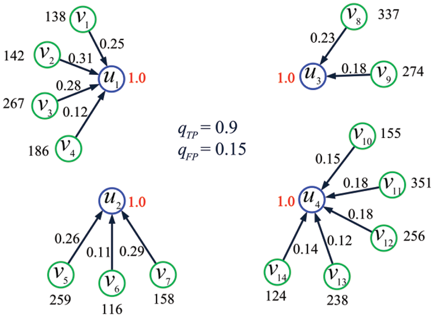
Figure 5: The IoT considered in Example 5

maxD(x)=axTsubject to bxT≤0.2,x∈[0,1]4,

where a=(0.2605,0.1868,0.1881,0.2647), b=(0.0349,0.0255,0.0303,0.0592). Since θ≥qFP, it follows from Theorem 1 that the linear program admits x∗=(1,1,1,1) as the unique optimal solution. Solving the linear program with MATLAB, we get this optimal solution.

Example 6. Consider the IoT shown in Fig. 6 and let θ=0.1. The corresponding ST model is

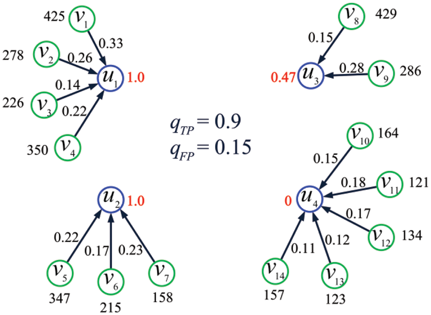
Figure 6: The IoT considered in Example 6

maxD(x)=axTsubject to bxT≤0.1,x∈[0,1]4,

where a=(0.4037,0.1876,0.1815,0.1272), b=(0.0533,0.0317,0.0317,0.0332). Since θ<qFP, a1/b1>a2/b2>a3/b3>a4/b4, it follows from Theorem 2 that the linear program admits x∗=(1,1,0.47,0) as the unique optimal solution. Solving the linear program with MATLAB, we get this optimal solution.

Example 7. Consider the IoT shown in Fig. 7 and let θ=0.1. The corresponding ST model is

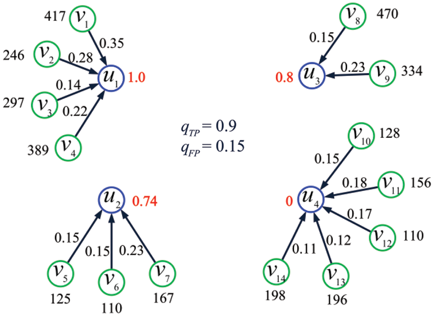
Figure 7: The IoT considered in Example 7

maxD(x)=axTsubject to bxT≤0.1,x∈[0,1]4,

where a=(0.4565,0.0983,0.1966,0.1485), b=(0.0566,0.0185,0.0369,0.0380). Since θ<qFP, a1/b1>a2/b2=a3/b3>a4/b4, it follows from Theorem 2 and Remark 6 that the linear program admits

S={x=(1,x2,x3,0):0≤x2,x3≤1,0.0185x2+0.0369x3=0.1}

as the set of optimal solutions. Solving the linear program with MATLAB, we get the optimal solution x∗=(1,0.74,0.8,0)∈S.

4.2 A Submodel of the ST Model

We refer to the ST model (8) satisfying ai/bi=c(1≤i≤N) as the RM* model. The following theorem provides a solution of this model.

Theorem 3. The linear program (8) with ai/bi=c (1≤i≤N) and θ<qFP admits

{x∈[0,1]N:axT=qTPqFPθ}

as the set of optimal solutions.

Proof. Since c=∑i=1Nai/∑i=1Nbi=qTP/qFP, we have bxT=qFP/qTPaxT. Hence, the linear program reduces to the following linear program:

maxD(x)=axTsubject to axT≤qTP/qFPθ,x∈[0,1]N.

The claim follows.

This theorem has the following useful corollary:

Corollary 1. The linear program (8) with rv=r(v∈V) and pv=p(v∈V) and θ<qFP admits

{x∈[0,1]N:axT=qTPqFPθ}

as the set of optimal solutions.

Proof. It is easily verified that ai/bi=qTP/qFP(1≤i≤N). The claim follows from Theorem 3.

Example 8. Consider the IoT shown in Fig. 8 and let θ=0.1. The corresponding linear program is

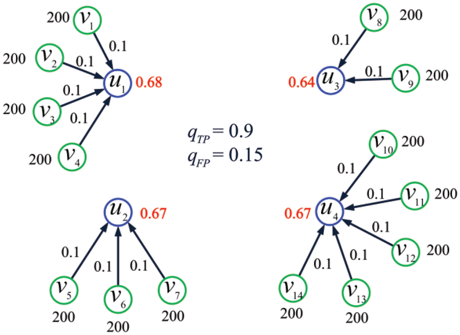
Figure 8: The IoT considered in Example 8

maxD(x)=axTsubject to bxT≤0.1,x∈[0,1]4,

where a=(0.2571,0.1929,0.1286,0.3214), b=(0.0429,0.0321,0.0214,0.0536). The two conditions in Corollary 1 are met. So, the linear program admits

S={x=(x1,x2,x3,x4)∈[0,1]4:0.2571x1+0.1929x2+0.1286x3+0.3214x4=0.6}

as the set of optimal solutions. Solving the linear program with MATLAB, we get the optimal solution x∗=(0.68,0.67,0.64,0.67)∈S.

5  Experiments

In the preceding section, we analytically resolved the ST model. In this section, we address the ST problem by employing a widely recognized network simulator, known as ns-3 [41].

5.1 The Layout of Three Two-Hop IoT

For our purpose, let us generate the layout of three two-hop IoT by following four steps as follows:

Step 1: For each of the three IoT, let all the radio model parameters be the same as those given in [42]. In particular, let the communication radius of a node be 80 m.

Step 2: The areas covered by the three IoT networks are square, with dimensions of 100 m ×100 m, 150 m × 150 m, and 200 m × 200 m, respectively. In each IoT network, the base station is positioned at the center of the corresponding square.

Step 3: The three IoT networks consist of 100, 300, and 500 nodes, respectively. In each scenario, the nodes are uniformly and randomly distributed within the respective square.

Step 4: A fraction of 5% nodes in each IoT network will serve as cluster heads. The LEACH routing protocol [42] will be employed to select the cluster heads and assign sensing nodes to each of the cluster heads. The topological structure of the three networks is shown in Fig. 9.

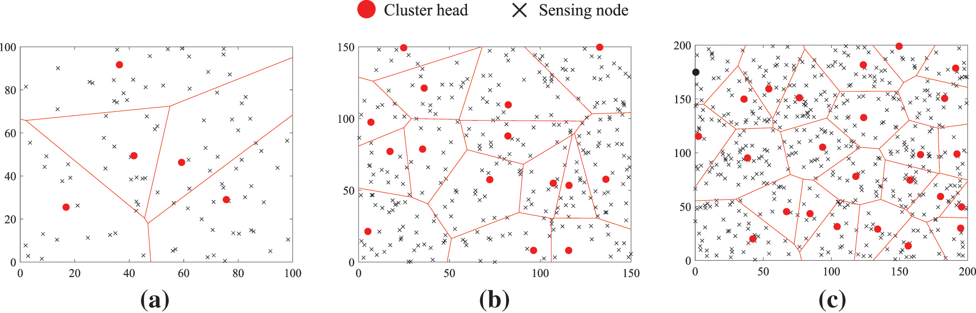
Figure 9: The layout of three two-hop IoT. Here, each of the three square areas is divided into a number of subfields, each of these subfields contains a single cluster head, and all the sensing nodes in the same subfield are routed to the cluster head located within the subfield

5.2 Experimental Results

Experiment 1. Consider the IoT layout shown in Fig. 9a. Let qTP=0.9, qFP=0.15, and θ=0.1. Generate a data-collecting scheme ℛ in this way: for each sensing node v, let rv be an integer chosen randomly and uniformly from the interval [100, 500], Generate a DT pattern 𝒫 in this way: for each sensing node v, let pv be a number chosen randomly and uniformly from the interval (0,0.2]. Now, we get a ST model. Solving the model with MATLAB, we get an optimal running mode of the ADS bank, denoted x∗, which is shown in Fig. 10a. Randomly and uniformly generate a set of 100 feasible running modes of the ADS bank, denoted X={xk:1≤k≤100}. Fig. 10b exhibits D(x), x∈X∪{x∗}. It is seen that D(x∗)>D(x),x∈X. This corroborates the optimality of the running mode x∗.

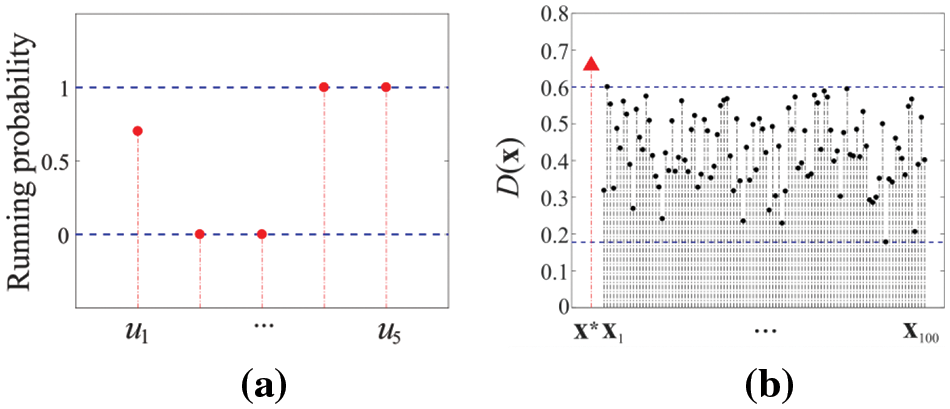
Figure 10: The results in Experiment 1: (a) the optimal running mode x∗, (b) a comparison of D(x∗) with D(x), x∈X

Experiment 2. Consider the IoT layout shown in Fig. 9b. Let qTP=0.9, qFP=0.15, and θ=0.1. Generate a data-collecting scheme ℛ in this way: for each sensing node v, let rv be an integer chosen randomly and uniformly from the interval [100, 500], Generate a DT pattern 𝒫 in this way: for each sensing node v, let pv be a number chosen randomly and uniformly from the interval (0,0.2]. Now, we get a ST model. Solving the model with MATLAB, we get an optimal running mode of the ADS bank, denoted x∗, which is displayed in Fig. 11a. Randomly and uniformly generate a set of 100 feasible running modes of the ADS bank, denoted X={xk:1≤k≤100}. Fig. 11b plots D(x),x∈X∪{x∗}. It is seen that D(x∗)>D(x),x∈X. This validates the optimality of the running mode x∗.

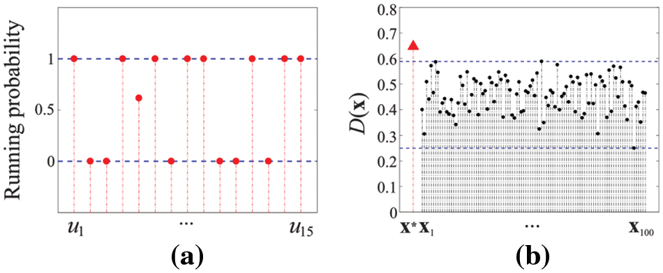
Figure 11: The results in Experiment 2: (a) the optimal running mode x∗, (b) a comparison of D(x∗) with D(x), x∈X

Experiment 3. Consider the IoT layout shown in Fig. 9c. Let qTP=0.9, qFP=0.15, and θ=0.1. Generate a data-collecting scheme ℛ in this way: for each sensing node v, let rv be an integer chosen randomly and uniformly from the interval [100, 500], Generate a DT pattern 𝒫 in this way: for each sensing node v, let pv be a number chosen randomly and uniformly from the interval (0, 0.2]. Now, we get a ST model. Solving the model with MATLAB, we get an optimal running mode of the ADS bank, denoted x∗, which is exhibited in Fig. 12a. Randomly and uniformly generate a set of 100 feasible running modes of the ADS bank, denoted X={xk:1≤k≤100}. Fig. 12b shows D(x), x∈X∪{x∗}. It is seen that D(x∗)>D(x), x∈X. This corroborates the optimality of the running mode x∗.

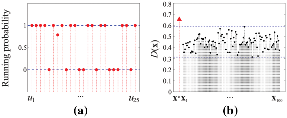
Figure 12: The results in Experiment 2: (a) the optimal running mode x∗, (b) a comparison of D(x∗) with D(x), x∈X

6  The Effect of Some Factors on the Maximum Combined Detection Rate

In this section, we discuss the effect of some factors on the maximum combined detection rate (i.e., the maximum value for the linear program (8)).

Theorem 4. Let Dmax denote the maximum value for the linear program (8). The following claims hold true:

(i) Dmax is increasing with θ.

(ii) Dmax is increasing linearly with qTP.

(iii) Dmax is decreasing with qFP.

Proof. (i) Consider a pair of linear programs as follows:

ℒ𝒫k=(U,𝒱,qTP,qFP,ℛ,𝒫,θk),k=1,2,

where θ1>θ2. Let Dkmax denote the maximum value for ℒ𝒫k,k=1,2. Since the objective functions of the two linear programs are identical, and the feasible set of ℒ𝒫1 includes that of ℒ𝒫2, we get D1max≥D2max. The claim is proven.

(ii) Consider a pair of linear programs as follows:

ℒ𝒫k=(U,𝒱,qTP(k),qFP,ℛ,𝒫,θ),k=1,2,(15)

where qTP(1)=α⋅qTP(2), α>1. Let Dkmax denote the maximum value for ℒ𝒫k, k=1,2. Let Dk(x) denote the objective function of ℒ𝒫k, k=1,2. Since the feasible sets of the two linear programs are identical, and D1(x)=α⋅D2(x), we get D1max=α⋅D2max. The claim is proven.

(iii) Consider a pair of linear programs as follows:

ℒ𝒫k=(U,𝒱,qTP,qFP(k),ℛ,𝒫,θ),k=1,2,(16)

where qFP(1)>qFP(2). Let Dkmax denote the maximum value for ℒ𝒫k, k=1,2. Since the objective functions of the two linear programs are identical, and the feasible set of ℒ𝒫1 is included in that of ℒ𝒫2, we get D1max≤D2max. The claim is proven.

This theorem is explained as follows. The first claim demonstrates that the maximum combined detection rate of the ADS bank can only be enhanced at the cost of an enhanced combined false alarm rate. The second claim tells us that enhancing the detection rate of a single ADS with a fixed false alarm rate is always helpful to enhance the maximum combined detection rate of the ADS bank. The third claim shows that reducing the false alarm rate of a single ADS with a fixed detection rate always contributes to the enhancement of the maximum combined detection rate of the ADS bank.

Example 9. Consider the IoT shown in Fig. 13 and let θ∈Θ={0.01,0.02,⋯,0.2}. The corresponding ST models are

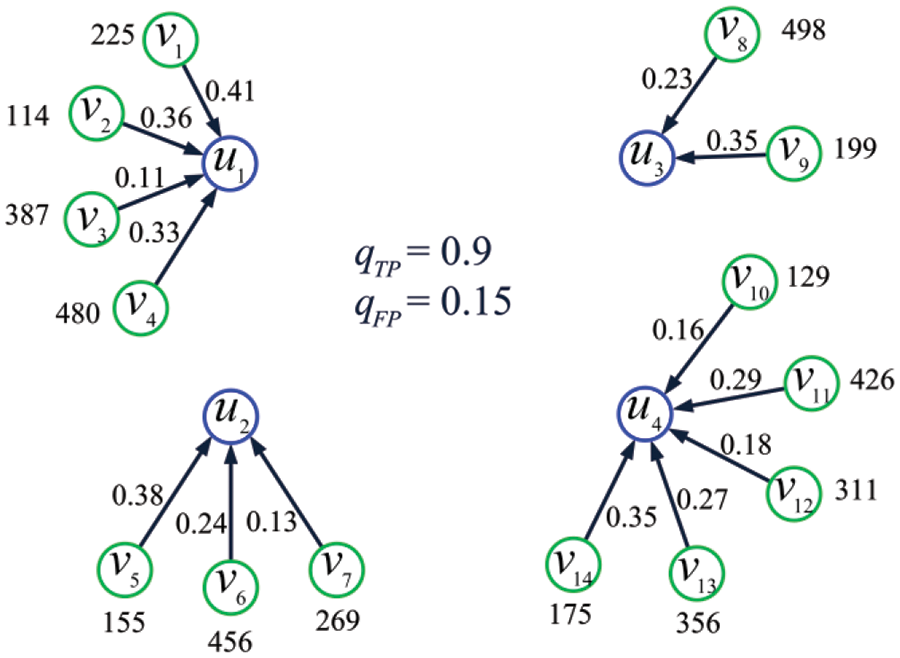
Figure 13: The IoT considered in Example 9

maxD(x)=axTsubject to bxT≤θ,x∈[0,1]4,

where a=(0.2787,0.1695,0.1536,0.2981), b=(0.0422,0.0327,0.0248,0.0503), and θ∈Θ. Solving the linear programs with MATLAB, we get their respective maximum values, denoted Dmax(θ),θ∈Θ. Fig. 14 shows Dmax(θ) vs. θ. It is evident that Dmax(θ) is increasing with θ, agreeing with Theorem 4(i). In particular, Dmax(θ)=qTP if θ≥qFP, conforming to Theorem 1.

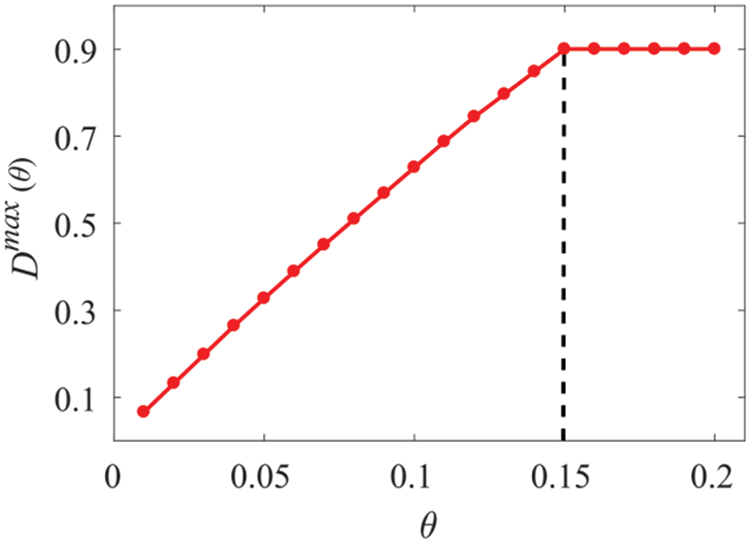
Figure 14: Dmax(θ) vs. θ for Example 9

Example 10. Consider the set of IoT shown in Fig. 15, where qTP∈Q={0.8,0.81,⋯,0.99}. Let θ=0.1. Then the corresponding linear programs are

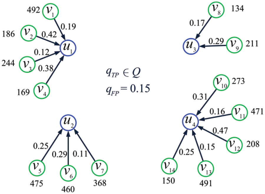
Figure 15: The set of IoT considered in Example 10

maxD(x)=a(qTP)xTsubject to bxT≤0.1,x∈[0,1]4,

where b=(0.037,0.047,0.012,0.055), a(qTP)=(0.2753qTP,0.2545qTP,0.0872qTP,0.3830qTP), qTP∈Q. Solving the linear programs with MATLAB, we get their respective maximum values, denoted Dmax(qTP), qTP∈Q. Fig. 16 shows Dmax(qTP) vs. qTP. It can be seen that Dmax(qTP) is increasing linearly with qTP, according with Theorem 4(ii).

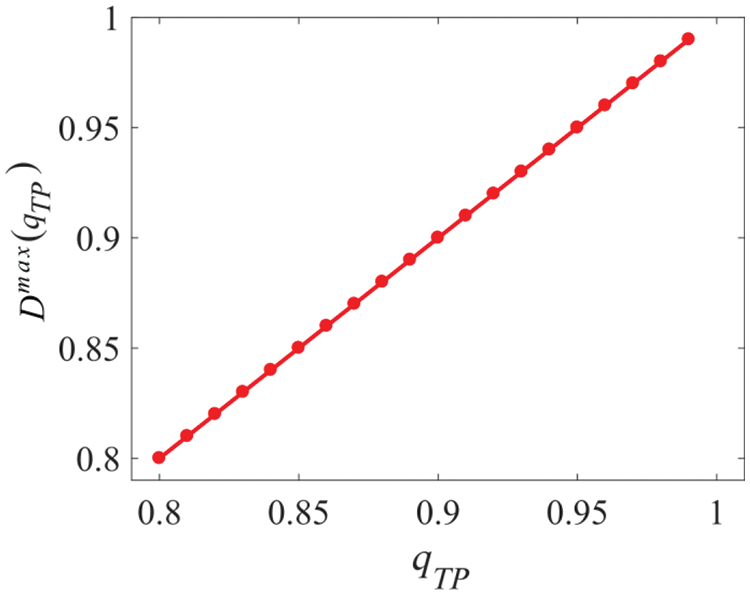
Figure 16: Dmax(qTP)vs. qTP for Example 10

Example 11. Consider the set of IoT shown in Fig. 17, where qFP∈Q={0.01,0.02,⋯,0.3}. Let θ=0.9. Then the corresponding linear programs are

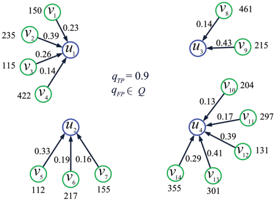
Figure 17: Dmax(qFP) vs. qFP for Example 11

maxD(x)=axTsubject to b(qFP)xT≤0.1,x∈[0,1]4,

where a=(0.233,0.112,0.170,0.385), b(qFP)=(0.2782qFP,0.1500qFP,0.2043qFP,0.3675qFP), qFP∈Q. Solving the linear programs with MATLAB, we get their respective maximum values, denoted Dmax(qFP), qFP∈Q. Fig. 18 shows Dmax(qFP) vs. qFP. The simulation results show that Dmax(qFP) is decreasing with qFP, in agreement with Theorem 4(iii). In particular, Dmax(qFP)=qTP if qFP≤θ, according with Theorem 1.

Figure 18: Dmax(qFP) vs. qFP for Example 11

Based on theoretical analysis and simulation results, we can summarize the following three key findings: (1) when the upper bound on the combined false alarm rate of the ADS bank is equal to or greater than the false alarm rate of an individual ADS, all ADSs in the ADS bank should be activated; (2) when the upper bound on the combined false alarm rate of the ADS bank is lower than the false alarm rate of an individual ADS, some ADSs in the ADS bank require activation, while others need to remain inactive, and the remaining ADSs are to be activated with a certain probability; (3) the maximum value of combined detection rate of the ADS bank is increasing with the upper bound of combined detection rate, increasing linearly with detection rate qTP, and decreasing with false alarm rate qFP.

7  Conclusion and Future Work

This paper has tackled the challenge of optimizing the performance of the anomaly detection system (ADS) network in a two-hop IoT environment. This problem has been modeled as a linear programming (i.e., the running mode (RM) model), which has been resolved analytically. This is the first time the defense of IoT against data-tampering attacks has been studied from a holistic perspective. The ADS management scheme proposed in this paper effectively resolves the issue of data unavailability caused by high false-positive rates in existing ADS algorithms.

In the future, several noteworthy issues merit investigation. Firstly, many real-world IoT systems operate with more than two hops, (real or false) data that pass through intermediate sensing nodes may be tampered with, which hinders the detection of false data. The study of the ST problem for multi-hop IoT poses a substantial challenge and merits comprehensive investigation. Secondly, the data-tampering pattern considered in this paper is assumed to be fixed. However, in practice, the data-tampering pattern is highly likely to vary over time. Under these circumstances, the ST model must be updated frequently to maximize the real combined detection rate of the ADS bank. In this situation, the choice of the update frequency is a problem. To characterize the data-tampering pattern, in the future, pattern recognition [43] may be used to further explore this issue. Thirdly, as blockchain technology [44] can be utilized to establish an anti-tampering mechanism, it holds tremendous potential in addressing DT attacks and warrants in-depth exploration. Furthermore, in the case where the network administrator of the IoT is strategic but the attacker is non-strategic, the ST problem may be studied through an optimal control approach [45]. Finally, in the case where the network administrator and the attacker are both strategic, it is appropriate to deal with the ST problem in the framework of game theory.

Acknowledgement: The authors would like to express their gratitude for the valuable feedback and suggestions provided by all the anonymous reviewers and the editorial team.

Funding Statement: This study was funded by the Chongqing Normal University Startup Foundation for PhD (22XLB021) and was also supported by the Open Research Project of the State Key Laboratory of Industrial Control Technology, Zhejiang University, China (No. ICT2023B40).

Author Contributions: The authors confirm contribution to the paper as follows: B. Liu: Methodology, Investigation, Software, Writing. Z. Zhang and S. Hu: Methodology, Investigation, Writing. S. Sun: Investigation, Writing-Original Draft, Writing-Review, Editing, and Funding. D. Liu and Z. Qiu: Resources, Validation, Writing-Review and Editing. All authors reviewed the results and approved the final version of the manuscript.

Availability of Data and Materials: Data supporting the findings of this study are available within the article.

Conflicts of Interest: The authors declare that they have no conflicts of interest to report regarding the present study.

References

1. M. A. Jamshed, K. Ali, Q. H. Abbasi, M. A. Imran, and M. Ur-Rehman, “Challenges, applications, and future of wireless sensors in Internet of Things: A review,” IEEE Sens. J., vol. 22, no. 6, pp. 5482–5494, 2022. doi: 10.1109/JSEN.2022.3148128. [Google Scholar] [CrossRef]

2. P. K. Malik et al., “Industrial Internet of Things and its applications in Industry 4.0: State of the art,” Comput. Commun., vol. 166, no. 5, pp. 125–139, 2021. doi: 10.1016/j.comcom.2020.11.016. [Google Scholar] [CrossRef]

3. A. E. Omolara et al., “The Internet of Things security: A survey encompassing unexplored areas and new insights,” Comput. Secur., vol. 112, no. 4, pp. 102494, 2022. doi: 10.1016/j.cose.2021.102494. [Google Scholar] [CrossRef]

4. L. P. Rondon, L. Babun, A. Aris, K. Akkaya, and A. S. Uluagac, “Survey on enterprise Internet-of-Things systems (E-IoTA security perspective,” Ad. Hoc Netw., vol. 125, no. 2, pp. 102728, 2022. doi: 10.1016/j.adhoc.2021.102728. [Google Scholar] [CrossRef]

5. H. K. Saini, M. Poriye, and N. Goyal, “A survey on security threats and network vulnerabilities in Internet of Things,” in Big Data Analytics in Intelligent IoT and Cyber-Physical Systems, Singapore: Springer Nature Singapore, 2023. [Google Scholar]

6. T. G. Lupu, “Main types of attacks in wireless sensor networks,” presented at the 2009 Int. Conf. Sig. Speech Img. Proc./Multimed. Int. Video Tech., Budapest, Hungary, Sept. 2009, pp. 180–185. [Google Scholar]

7. A. I. A. Ahmed, S. H. Ab Hamid, A. Gani, and M. K. Khan, “Trust and reputation for Internet of Things: Fundamentals, taxonomy, and open research challenges,” J. Netw. Comput. Appl., vol. 145, no. 5, pp. 102409, 2019. doi: 10.1016/j.jnca.2019.102409. [Google Scholar] [CrossRef]

8. J. Bi, F. Luo, G. Liang, X. Yang, S. He and Z. Y. Dong, “Impact assessment and defense for smart grids with FDIA against AMI,” IEEE Trans. Netw. Sci. Eng., vol. 10, no. 2, pp. 578–591, 2022. doi: 10.1109/TNSE.2022.3197682. [Google Scholar] [CrossRef]

9. M. Serror, S. Hack, M. Henze, M. Schuba, and K. Wehrle, “Challenges and opportunities in securing the industrial internet of things,” IEEE Trans. Ind. Inform., vol. 17, no. 5, pp. 2985–2996, 2020. [Google Scholar]

10. J. Bi, S. He, F. Luo, W. Meng, L. Ji and D. W. Huang, “Defense of advanced persistent threat on industrial internet of things with lateral movement modelling,” IEEE Trans. Ind. Inform., vol. 19, no. 9, pp. 9619–9630, 2022. doi: 10.1109/TII.2022.3231406. [Google Scholar] [CrossRef]

11. D. W. Huang, W. Liu, and J. Bi, “Data tampering attacks diagnosis in dynamic wireless sensor networks,” Comput. Commun., vol. 172, no. 3, pp. 84–92, 2021. doi: 10.1016/j.comcom.2021.03.007. [Google Scholar] [CrossRef]

12. J. Giraldo, M. E. Hariri, and M. Parvania, “Decentralized moving target defense for microgrid protection against false-data injection attacks,” IEEE Trans. Smart Grid, vol. 13, no. 5, pp. 3700–3710, 2022. doi: 10.1109/TSG.2022.3176246. [Google Scholar] [CrossRef]

13. A. Kumar, S. Sharma, N. Goyal, A. Singh, X. Cheng and P. Singh, “Secure and energy-efficient smart building architecture with emerging technology IoT,” Comput. Commun., vol. 176, pp. 207–217, 2021. [Google Scholar]

14. L. Kakkar et al., “A secure and efficient signature scheme for IoT in healthcare,” Comput. Mater. Contin, vol. 73, no. 3, pp. 6151–6168, 2022. [Google Scholar]

15. M. Xie, S. Han, B. Tian, and S. Parvin, “Anomaly detection in wireless sensor networks: A survey,” J. Netw. Comput. Appl., vol. 34, no. 4, pp. 1302–1325, 2011. [Google Scholar]

16. I. Butun, S. D. Morgera, and R. Sankar, “A survey of intrusion detection systems in wireless sensor networks,” IEEE Commun. Surv. Tutor., vol. 16, no. 1, pp. 266–282, 2014. [Google Scholar]

17. G. Q. Xie, L. T. Yang, Y. Yang, H. Luo, R. Li and M. Alazab, “Threat analysis for automotive CAN networks: A GAN model-based intrusion detection technique,” IEEE Trans. Intell. Transp., vol. 22, no. 7, pp. 4467–4477, 2021. [Google Scholar]

18. B. Subba, S. Biswas, and S. Karmakar, “Intrusion detection in mobile ad-hoc networks: Bayesian game formulation,” Eng. Sci. Technol. Int. J., vol. 19, no. 2, pp. 782–799, 2016. doi: 10.1016/j.jestch.2015.11.001. [Google Scholar] [CrossRef]

19. K. Wang, M. Du, D. Yang, C. Zhu, J. Shen and Y. Zhang, “Game-theory-based active defense for intrusion detection in cyber-physical embedded systems,” ACM Trans. Embed. Comput. Syst., vol. 16, no. 1, pp. 1–21, 2016. [Google Scholar]

20. S. Shen, L. Huang, H. Zhou, S. Yu, E. Fan and Q. Cao, “Multistage signaling game-based optimal detection strategies for suppressing malware diffusion in fog-cloud-based IoT networks,” IEEE Internet Things, vol. 5, no. 2, pp. 1043–1054, 2018. doi: 10.1109/JIOT.2018.2795549. [Google Scholar] [CrossRef]

21. I. Onat and A. Miri, “An intrusion detection system for wireless sensor networks,” presented at the 2005 IEEE Int. Conf. Wireless Mobile Comput. Netw. Commun., Montreal, Canada, Aug. 2005, pp. 253–259. [Google Scholar]

22. S. Rajasegarar, C. Leckie, and M. Palaniswami, “Anomaly detection in wireless sensor networks,” IEEE Wirel. Commun., vol. 15, no. 4, pp. 34–40, 2008. doi: 10.1109/MWC.2008.4599219. [Google Scholar] [CrossRef]

23. S. Wang, W. Xu, and Y. Liu, “Res-TranBiLSTM: An intelligent approach for intrusion detection in the Internet of Things,” Comput. Netw., vol. 235, pp. 109982, 2023. [Google Scholar]

24. H. Asgharzadeh, A. Ghaffari, M. Masdari, and F. S. Gharehchopogh, “Anomaly-based intrusion detection system in the Internet of Things using a convolutional neural network and multi-objective enhanced capuchin search algorithm,” J. Parallel Distr. Comput., vol. 175, pp. 1–21, 2023. [Google Scholar]

25. K. Yang, Y. Shi, Z. Yu, Q. Yang, A. K. Sangaiah and H. Zeng, “Stacked one-class broad learning system for intrusion detection in Industry 4. 0,” IEEE Trans. Ind. Inform., vol. 19, no. 1, pp. 251–260, 2023. [Google Scholar]

26. A. Abduvaliyev, A. K. Pathan, J. Zhou, R. Roman, and W. C. Wong, “On the vital areas of intrusion detection systems in wireless sensor networks,” IEEE Commun. Surv. Tutor., vol. 15, no. 3, pp. 1223–1237, 2013. [Google Scholar]

27. F. Liu, X. Cheng, and D. Chen, “Insider attacker detection in wireless sensor networks,” presented at the 26th IEEE Int. Conf. Comput. Commun., Washington DC, USA, May 2007, pp. 1937–1945. [Google Scholar]

28. R. Kumar, P. Kumar, R. Tripathi, G. P. Gupta, S. Garg and M. M. Hassan, “A distributed intrusion detection system to detect DDoS attacks in blockchain-enabled IoT network,” J. Parallel Distr. Comput., vol. 164, pp. 55–68, 2022. [Google Scholar]

29. B. Li, R. Lu, W. Wang, and K. R. Choo, “Distributed host-based collaborative detection for false data injection attacks in smart grid cyber-physical system,” J. Parallel Distr. Comput., vol. 103, pp. 32–41, 2017. [Google Scholar]

30. Q. Zhu, C. Fung, R. Boutaba, and T. Basar, “GUIDEX: A game-theoretic incentive-based mechanism for intrusion detection networks,” IEEE J. Sel. Areas Commun., vol. 30, no. 11, pp. 2220–2230, 2012. doi: 10.1109/JSAC.2012.121214. [Google Scholar] [CrossRef]

31. H. Wu and W. Wang, “A game theory based collaborative security detection method for internet of things systems,” IEEE Trans. Inf. Foren. Secur., vol. 13, no. 6, pp. 1432–1445, 2018. doi: 10.1109/TIFS.2018.2790382. [Google Scholar] [CrossRef]

32. D. W. Huang, F. Luo, J. Bi, and M. Sun, “An efficient hybrid IDS deployment architecture for multi-hop clustered wireless sensor networks,” IEEE Trans. Inf. Foren. Secur., vol. 17, pp. 2688–2702, 2022. doi: 10.1109/TIFS.2022.3191491. [Google Scholar] [CrossRef]

33. H. Wang, Z. Yuan, and C. Wang, “Intrusion detection for wireless sensor networks based on multi-agent and refined clustering,” in 2009 WRI Int. Conf. Commun. Mobile Comput., Kunming, China, Jan. 2009, pp. 450–454. [Google Scholar]

34. S. Shin, T. Kwon, G. Y. Jo, Y. Park, and H. Rhy, “An experimental study of hierarchical intrusion detection for wireless industrial sensor networks,” IEEE Trans. Ind. Inform., vol. 6, no. 4, pp. 744–757, 2010. doi: 10.1109/TII.2010.2051556. [Google Scholar] [CrossRef]

35. A. Mehmood, A. Khanan, M. M. Umar, S. Abdullah, K. A. Z. Ariffin and H. Song, “Secure knowledge and cluster-based intrusion detection mechanism for smart wireless sensor networks,” IEEE Access, vol. 6, pp. 5688–5694, 2018. doi: 10.1109/ACCESS.2017.2770020. [Google Scholar] [CrossRef]

36. Y. Zhang, N. Meratnia, and P. J. Havinga, “Outlier detection techniques for wireless sensor networks: A survey,” IEEE Commun. Surv.; Tutor., vol. 12, no. 2, pp. 159–170, 2010. [Google Scholar]

37. S. S. Wang, K. Q. Yan, S. C. Wang, and C. W. Liu, “An integrated intrusion detection system for cluster-based wireless sensor networks,” Expert Syst. Appl., vol. 38, no. 12, pp. 234– 243, 2011. [Google Scholar]

38. S. Rajasegarar, C. Leckie, and M. Palaniswami, “Hyperspherical cluster based distributed anomaly detection in wireless sensor networks,” J. Parallel Distr. Comput., vol. 74, no. 1, pp. 1833–1847, 2014. [Google Scholar]

39. P. Chen, S. Yang, and J. A. McCann, “Distributed real-time anomaly detection in networked industrial sensing systems,” IEEE Trans. Ind. Electron., vol. 62, no. 6, pp. 3832–3842, 2015. [Google Scholar]

40. A. Mabrouk and A. Naja, “Intrusion detection game for ubiquitous security in vehicular networks: A signaling game based approach,” Comput. Netw., vol. 225, pp. 109649, 2023. [Google Scholar]

41. G. F. Riley and T. R. Henderson, “The ns-3 network simulator,” in Modeling and Tools for Network Simulation, Berlin, Heidelberg: Springer, 2010. [Google Scholar]

42. W. B. Heinzelman, A. P. Chandrakasan, and H. Balakrishnan, “An application-specific protocol architecture for wireless microsensor networks,” IEEE Trans. Wirel. Commun., vol. 1, no. 4, pp. 660–670, 2002. doi: 10.1109/TWC.2002.804190. [Google Scholar] [CrossRef]

43. C. Zhu, K. Yang, Q. Yang, Y. Pu, and C. L. P. Chen, “A comprehensive bibliometric analysis of signal processing and pattern recognition based on distributed optical fiber,” Meas., vol. 206, no. 4, pp. 112340, 2023. doi: 10.1016/j.measurement.2022.112340. [Google Scholar] [CrossRef]

44. B. S. Egala, A. K. Pradhan, V. Badarla, and S. P. Mohanty, “Fortified-chain: A blockchain-based framework for security and privacy-assured internet of medical things with effective access control,” IEEE Internet Things, vol. 8, no. 14, pp. 11717–11731, 2021. doi: 10.1109/JIOT.2021.3058946. [Google Scholar] [CrossRef]

45. S. P. Sethi, What is Optimal Control Theory?, Cham, Switzerland: Springer, 2019. [Google Scholar]