An Enhanced Multiview Transformer for Population Density Estimation Using Cellular Mobility Data in Smart City

1  Introduction

In recent years, the prevalence of wireless communication devices, such as smartphones, has significantly increased. As of 2019, there were 3.5 billion smartphone users globally, accounting for 42.63% of the world’s population [1]. The rapid expansion of mobile communication services has led to the accumulation of massive amounts of system logs and paperless office data by mobile communication operators. We collectively refer to this data as cellular station data, which includes temporal and spatial user information and can accurately reflect the number of people at a specific time and location [2–6]. By utilizing this information, we can estimate changes in the number of people in a particular area and study urban population movement and approximate activity trajectories.

Population density is a critical measure for urban traffic management [7]. It can be analyzed using base station signaling data to predict future changes. These predictions offer valuable information for urban planning [8], traffic management, industry applications, and social security [9]. For instance, subway station locations can be planned based on population density distribution and movement [10]. Traffic load predictions can inform government traffic management [11]. Forecasting crowd movements can assist venue managers, such as those at banks and shopping centers, to prepare in advance. This preparation can reduce customer waiting times and increase service levels and management efficiency [12]. In the context of social security, predictions can be made about possible abnormal events using base station data, population density distribution, and crowd movement information [13]. These predictions allow for preemptive measures to be taken [14]. In conclusion, predicting population density over time enables us to identify and address potential social and security risks early. It enhances urban operation and management efficiency and contributes to social and economic development.

Currently, many traditional neural network models are employed for short-term time-series prediction on conventional datasets [11,15–19]. Concurrently, Transformer-based models have been introduced to capture long-term dependencies in traditional time-series forecasting and have shown promising results [20–23].

To enhance the rationality and effectiveness of base station and population data, we need to preprocess the raw cellular station data [24]. However, we found that the preprocessing methods and steps in existing research are incomplete and lack systematic descriptions. On the other hand, current population prediction methods mostly consider short-term time series predictions and cannot predict long-term trends in population changes. In addition, some existing long-term prediction models fail to fully capture the high-frequency change characteristics of population numbers, leading to insufficient optimization of local high-frequency changes in population numbers. These models continue to fall short in capturing characteristics of high-frequency changes in time-series data predictions based on variations in population size.

To address these problems, we first propose a complete base station data preprocessing method, including five steps: removing abnormal invalid data, duplicate data, ping-pong data, abnormal drift data, and organizing and counting data according to certain time slices. Then, we chose the Transformer-based model for population density prediction to solve the problem of long-term time series prediction of population density. In addition, we designed a multi-view module embedded in the time-domain or frequency-domain based Transformer model to capture the local high-frequency change characteristics of population numbers, thereby improving the prediction accuracy of the Transformer baseline model. We propose a multi-view mechanism to enhance the capturing rate of high-frequency variation patterns by combining both time-domain and frequency-domain signals in the data.

In summary, the main contributions of this paper are as follows:

1.    We propose a comprehensive cellular data station data preprocessing method that processes temporal and spatial information, providing a reliable data foundation for subsequent population prediction.

2.    We design a multi-view enhancement model based on the Transformer, dubbed MVformer. By introducing the time-domain based Transformer structure and frequency-domain enhancement techniques, we effectively improve the accuracy of long-term time series population prediction.

3.    Through experimental verification, our model demonstrates good performance in population prediction tasks, proving the model’s effectiveness and feasibility.

These contributions have a driving effect on the study of base station data in population prediction and related fields, providing strong support and decision-making basis for urban planning, traffic management, industry applications, and social security, among other fields. At the same time, the methods and experimental results of this paper provide references for future related research.

2  Related Work

This study primarily aims to predict urban population density, particularly forecasting future trends of these changes. The handling of temporal information is crucial in our prediction model. This aligns with the growing interest in temporal prediction in the machine learning and artificial intelligence fields. Significant research over the past few years has been devoted to improving temporal prediction models.

2.1 Traditional Machine Learning Methods

Traditional models often employ statistical methods. One such method is the Autoregressive Integrated Moving Average (ARIMA) model. Ho et al. [25] proposed this model for the reliable temporal prediction of repairable systems. Another method is the autoregressive (AR) models, which have been applied to time series forecasting. Bergmeir et al. [26] demonstrated this application using K-fold cross-validation. Additionally, Roy et al. [27] proposed the use of the Least Absolute Shrinkage and Selection Operator (LASSO) in linear regression. They used this method for predicting stock trends.

However, these traditional methods cannot capture complex temporal patterns effectively. Therefore, researchers have started exploring the use of Neural Network models for time series pattern learning and prediction.

2.2 Recurrent Neural Networks (RNN) Based Methods

In recent years, with the advancement of deep learning technologies, more and more researchers have applied them to temporal prediction. For example, Siami-Namini et al. [15] found that compared with ARIMA, Long Short-Term Memory (LSTM) networks based on Recurrent Neural Networks (RNN) can significantly reduce the error rate and improve the prediction accuracy in temporal prediction tasks. Chung et al. [16] used LSTM units and Gated Recurrent Units (GRU) in RNNs to complete tasks such as speech signal modeling and other temporal signal construction tasks, achieving good results. Zhang et al. [17] based their work on the GRU neural network and used Fourier Cycle Decomposition (FCD) to decompose the time series into trend, cycle, and residual sub-sequences for training and forecasting in the temporal prediction model.

2.3 Convolutional Neural Networks (CNN) Based Methods

In short-term temporal prediction, besides RNN models, Convolutional Neural Networks (CNN) have also been widely applied. Koprinska et al. [18] used CNN in energy time series prediction tasks, yielding good results. Bai et al. [19] conducted a systematic evaluation of generic convolutional and recursive architectures for sequence modeling and found that simple convolutional architectures outperform typical recurrent networks on different tasks and datasets. They proposed a generic Temporal Convolutional Network (TCN). Yadav et al. [28] proposed a deep learning model that combines a multi-layer LSTM structure with multiple parallel CNN modules. This model aims to capture long-term dependencies in time series data and extract both local and global features for improving the accuracy of predicting future trends and patterns in time series data.

2.4 Graph Neural Networks (GNN) Based Methods

Jiang et al. [29,30] highlighted that Graph Neural Networks (GNNs) have emerged as a viable solution in various traffic forecasting problems, owing to their exceptional compatibility with traffic systems characterized by graph structures. For the temporal prediction task of traffic flow, Yu et al. [11] proposed a Spatio-Temporal Graph Convolutional Network (STGCN) model. This model considers the dependencies of space and time and effectively captures the spatio-temporal correlation of traffic flow. Ling et al. [31] proposed a network traffic prediction model based on Graph Convolution Network (GNN) to generate network traffic distribution for efficient edge server placement, resulting in significant reductions in cost and overloading of edge servers in a 5G network.

2.5 Transformer Based Long-Term Temporal Prediction Methods

The models above have achieved good results in short-term forecasting tasks. However, their performance in capturing long-term temporal patterns is suboptimal. To address this issue, researchers have developed Transformer-based time series prediction models specifically designed for long-term temporal prediction tasks. For long-term temporal prediction tasks, the Transformer model proposed by Vaswani et al. [20] can capture the relationships between different positions in a sequence. This model adopts an encoder-decoder structure and self-attention mechanism, effectively capturing the temporal characteristics of time series. Based on the Transformer model, Li et al. [21] completed time series prediction tasks. To solve the problem of the Transformer in handling complex time patterns and information utilization bottlenecks, Wu et al. [22] proposed an Autoformer model based on a deep decomposition architecture and self-correlation mechanism. The FEDFormer model proposed by Zhou et al. [23] adopts a Frequency Enhanced Decomposition (FED) approach, performing long-term temporal prediction tasks through Fourier transform analysis of time series in the frequency domain. The Transformer-based time series prediction models have achieved good results in generic long-term prediction tasks. However, these models still cannot capture the characteristics of high-frequency variations in time series prediction tasks based on population changes. Consequently, we propose the mechanism of multi-view in this paper and enhance the detection rate of high-frequency variation rules by combining time-domain signals and frequency-domain signals from the data.

3  Dataset Introduction and Preprocessing

In this section, we will elaborate on the base station dataset used in this research and its preprocessing steps.

3.1 Dataset Description

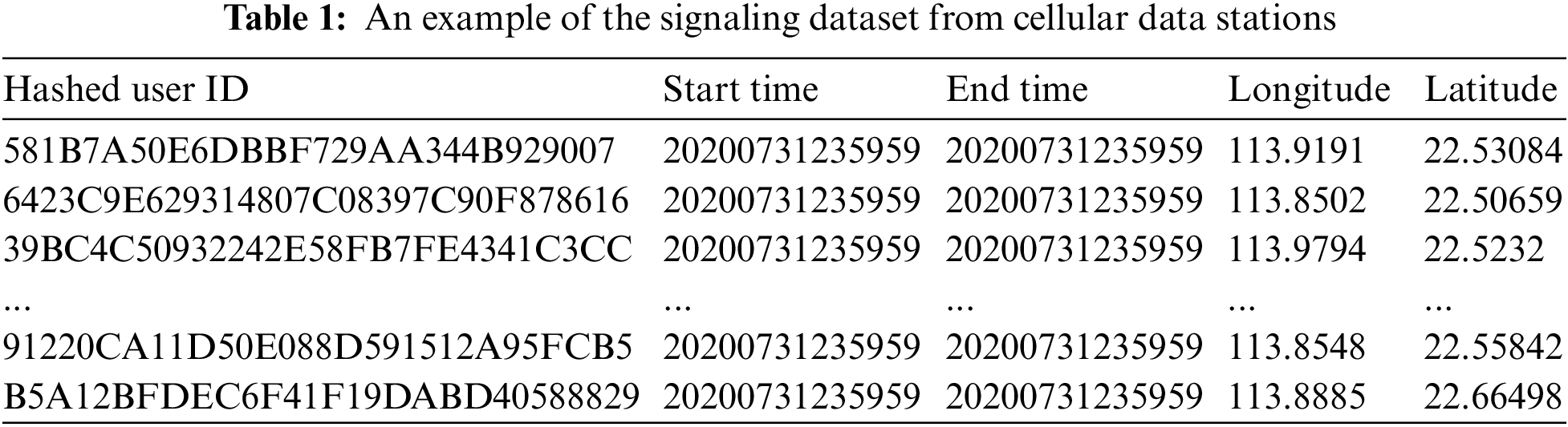
Our dataset is provided by a mobile communication service provider located in Shenzhen, a major city in China, and includes anonymized base station signaling data collected from August 01 to August 31, 2020. Each piece of signaling data is a quintuple, containing user ID, start time, end time, base station longitude, and base station latitude. The dataset we received comprises about 7.8 million users (including roaming users from other regions). The dataset is divided into 31 files, corresponding to each day of August 2020. Each file is approximately 3 GB after compression, totaling about 100 GB. An example of the signaling dataset is shown in Table 1.

3.2 Dataset Preprocessing

Since the original base station data is vast and contains a large amount of invalid data, these could negatively impact the subsequent population density prediction task. For instance, invalid duplicate data could lead to the overcounting of crowd numbers at specific times and places. Furthermore, “ping-pong” data and “drift” data in the base station signaling data could cause erroneous crowd counting. To enhance the usability and accuracy of the data, we performed preprocessing on the original base station data.

3.2.1 Removal of Abnormal Invalid Data

Invalid data refers to data that does not conform to the format listed in Table 1. During the data collection process, it is possible for certain anomalous and invalid data to be produced. Such anomalies can arise from issues such as cellular base station malfunctions or transmission errors. The presence of these anomalous and invalid data points can have a detrimental impact on subsequent data analysis and modeling, and therefore, it becomes necessary to remove them. The purpose of this step is to improve the overall quality and accuracy of the data, enabling subsequent analyses to be conducted in a more reliable and effective manner. We identify and remove invalid data by checking whether each field of every data entry adheres to the specified format and whether the number of fields is correct.

3.2.2 Sorting the Signaling Data by User ID

After removing the invalid data caused by technical issues, we need to sort the original data based on user IDs to facilitate subsequent preprocessing steps. However, due to the large scale of the data, the time and space costs of directly sorting the original data are unacceptable. Therefore, we chose to use a block processing method. First, we distributed the data into 4096 different files based on the first three digits of the user IDs. Then, we used a multi-process parallel processing approach to sort the records in these files by user ID and time. In this way, we obtained base station signaling data sorted by user ID.

3.2.3 Removal of Duplicate Data

In the base station signaling data, duplicate data refers to data with the same user ID and base station coordinates within the same time period. The purpose of this step is to remove duplicate data that have identical timestamps and location information. These duplicate data may be caused by instrument malfunctions, errors in data acquisition devices, or other factors. These duplicate data could lead to statistical errors in crowd numbers, as the same user might be counted multiple times. Deleting duplicate data helps to ensure that our analysis results are not influenced by repeated observations and reduces redundant calculations in subsequent data processing steps. Therefore, we need to read the sorted signaling data from the previous step, identify, and remove duplicate data within the same time slice.

3.2.4 Removal of Ping-Pong Data

In the context of base station signaling data, ping-pong data refers to the situation where a user frequently switches between two base stations within a short period of time. This typically occurs when a user is located at the boundary between two base stations, as shown in Fig. 1. The presence of ping-pong data can result in a user being counted multiple times, leading to inaccuracies in analysis results and introducing bias. As ping-pong data does not represent the actual behavior of the base stations, it can also affect the subsequent processing of crowd density data. Therefore, we eliminate ping-pong data by examining the frequency of time-based switching and the hopping of connections in the data. We extract the sorted and deduplicated signaling data from the previous step, identify and remove ping-pong data that occurs within a 10-min interval. This helps ensure the continuity and consistency of the data, reduces statistical bias caused by ping-pong data, and improves the reliability of subsequent analysis. The pseudocode description of the ping-pong data processing procedure can be found in Algorithm 1.

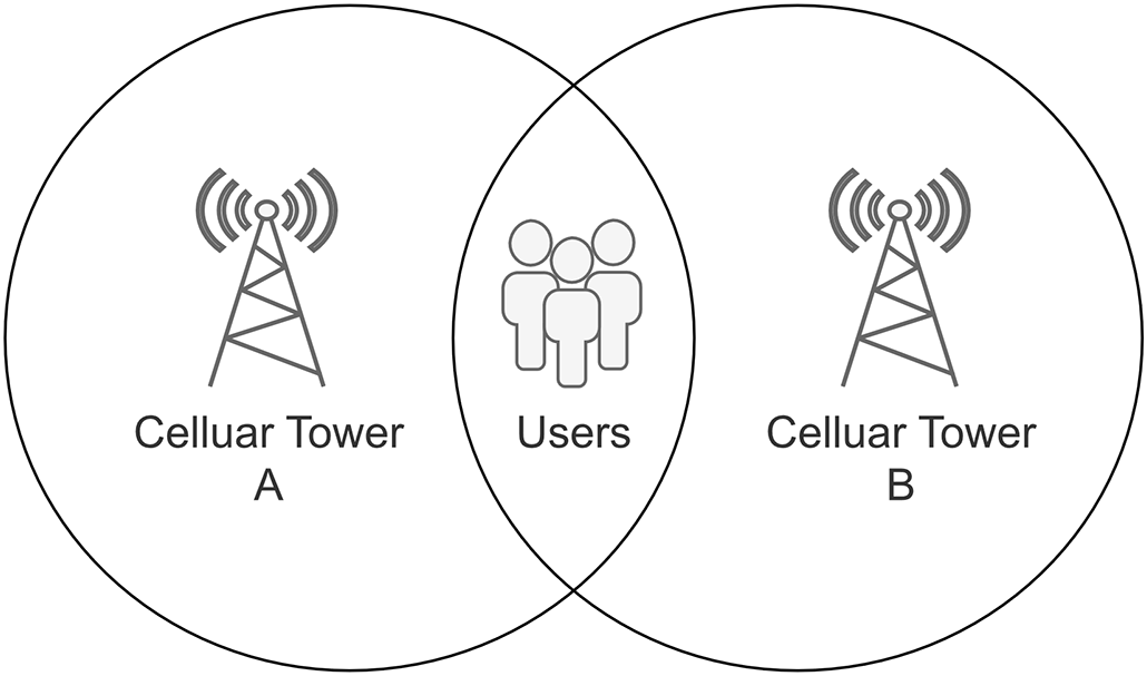
Figure 1: Ping-pong data occurrence schematic diagram. Ping-pong data may be generated when a user is located at the border of the coverage area of two cellular data stations

3.2.5 Removal of Abnormal Drift Data

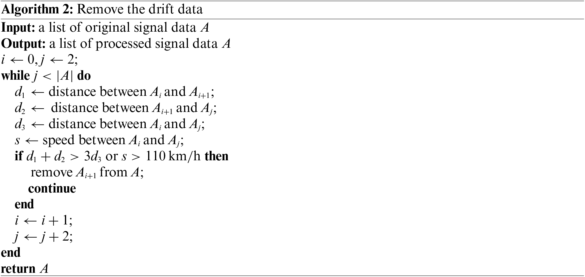
Abnormal drift data refers to situations in which a user’s consecutive signaling data shows that the user has moved a significant distance in a short period of time, as illustrated in Fig. 2. This can occur when the user is in an environment that interferes with the reception of the mobile signal, resulting in sudden changes in the recorded user location at the base station, among other abnormal behaviors. These deviations can stem from environmental changes, equipment malfunction, or other causes. The presence of such drift data can lead to inaccurate analysis results and distort our understanding of network performance and behavior. Therefore, it is essential to handle such data, eliminating the impact of these temporary anomalies to ensure the authenticity and rationality of the data, thereby improving the accuracy of data analysis. To address this issue, we have adopted specific thresholds and statistical rules to detect and remove these abnormal drift data. The specific steps of the abnormal drift data handling process are described in pseudocode in Algorithm 2.

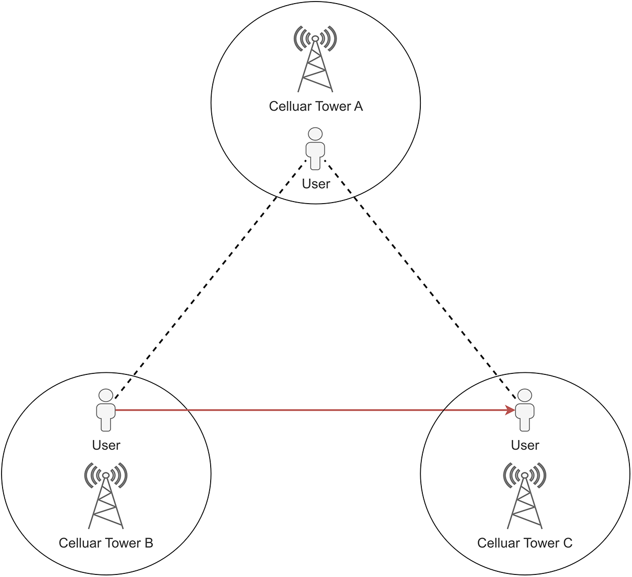
Figure 2: A schematic diagram suggesting reasons for the occurrence of abnormal drift data. Abnormal drift data may be generated when a user moves a large distance within a short time

After the aforementioned data processing steps, we organized and counted the base station signaling data at intervals of five minutes, resulting in a time series dataset of base station signals. Slicing data by time allows for a more structured organization of data and enables data analysis based on different time periods. This approach is beneficial for identifying the temporal correlation and periodicity of data, particularly in predicting population quantities. Additionally, it provides a more comprehensive and targeted foundation for subsequent analysis. First, we performed a time-dimension visualization analysis on these data and discovered clear regularities at three different time scales: daily, weekly, and monthly.

Fig. 3 shows the distribution of base station signaling quantities on August 03, 2020 (Monday). It can be clearly seen that the number of signals strongly correlates with human daily activity patterns. During the day, the number of signals is high, while at midnight, the number of signals significantly decreases. In addition, there are two peak periods for the number of signals each day: one around 8 am and another around 7 pm. In Fig. 4, we can also see these two peak periods on weekdays.

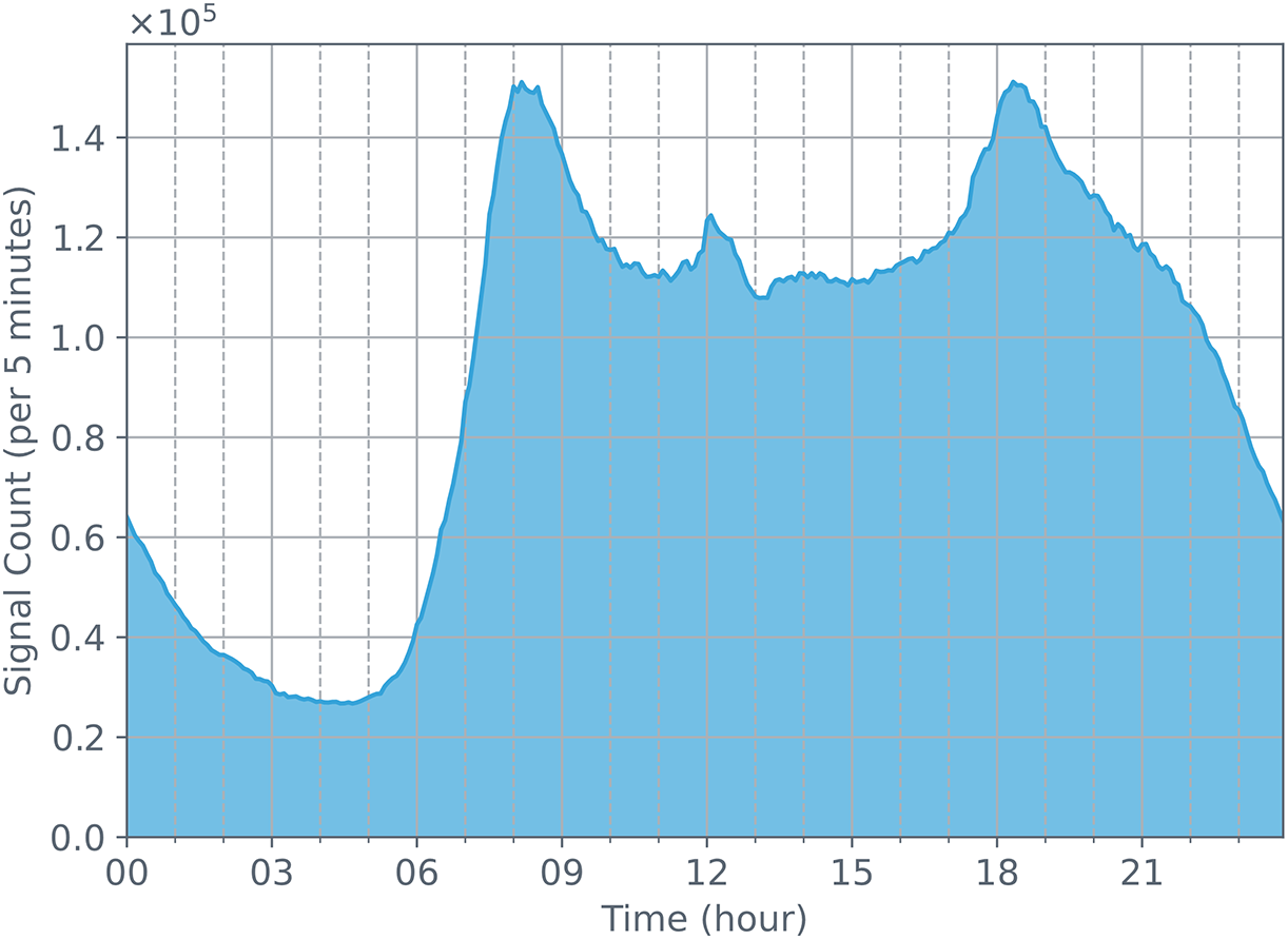
Figure 3: The changes in the number of cellular data station signals detected on August 03, 2020

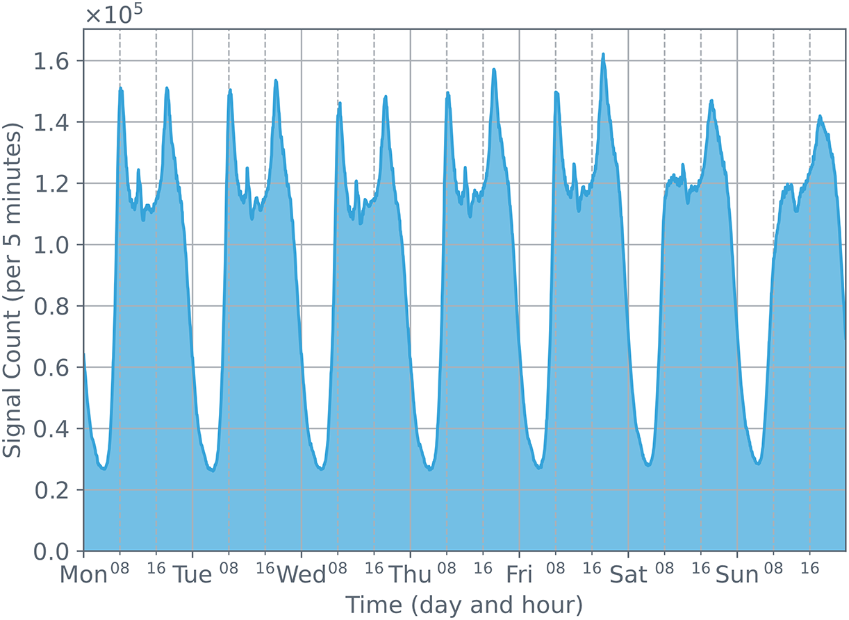
Figure 4: The changes in the number of cellular data station signals detected over a week. It can be observed that the changes have a strong daily periodicity

Fig. 4 describes the distribution of base station signaling quantities from August 03, 2020, to August 09, 2020. Fig. 5 shows the distribution of base station signaling quantities from August 01, 2020, to August 31, 2020. From these two figures, we can clearly see that the base station signaling data presents a cyclical pattern on a weekly timescale, and the number of signals on weekends is less than on weekdays. These variations in the number of signals primarily stem from people’s weekly work and life arrangements.

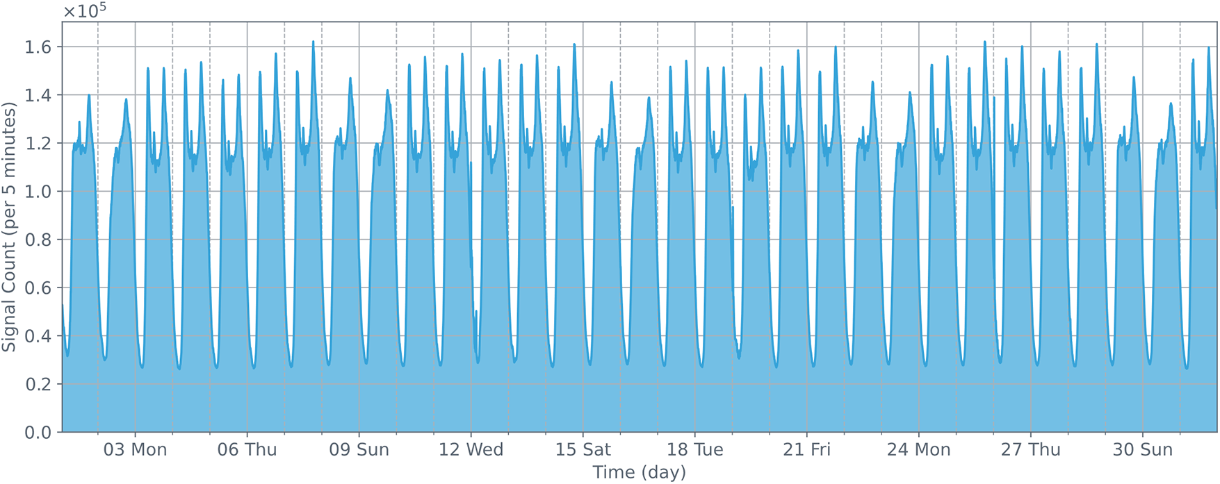
Figure 5: The changes in the number of cellular data station signals detected within a month. It can be observed that the changes display a periodicity on a weekly basis

To facilitate regional population prediction based on base station signaling data, it is necessary to partition the area according to certain rules. Past related studies have mostly adopted fixed-size grid partitioning. However, this partitioning method may lead to the inclusion of areas where no signals are generated within the prediction scope, and grids spanning multiple areas may lack practical significance in prediction [32]. Meanwhile, manual partitioning may render the prediction work lacking in universality and portability. Therefore, in this study, we choose to use a clustering method to cluster all base stations that generate signaling data using the K-Means algorithm. Based on the Elbow rule, we calculate the intra-cluster distance of base stations under different K values. Ultimately, we set K to 30, which means we divide all base stations into 30 categories based on their longitude and latitude, serving as 30 prediction regions.

Finally, we organize the original base station signaling data according to five-minute time slots and tag each base station signaling data with its corresponding research region ID. The start time in the original base station data is precise to the second, but in actual time series prediction tasks, we do not need such precise time slots. Therefore, during data preprocessing, we can organize crowd number data by time slots and mark the region ID to which the base station data belongs according to the partitioned areas. Ultimately, we count the crowd number data in different regions based on the region ID and corresponding time slot number to obtain the crowd number dataset for time series prediction.

4  Crowd Prediction Model

To more effectively predict the number of people in each area using base station signaling data, we designed a crowd number prediction model called Multi-View Transformer (MVformer). Firstly, our MVformer model is based on Transformer, a neural network model with self-attention mechanism that has a powerful ability to capture long-range dependencies in sequences. Secondly, the MVformer model combines multi-view modules and cross-view attention modules to better utilize the information among different views. The schematic diagram of the model is shown in Fig. 6. The multi-view modules are responsible for extracting and integrating features, while the cross-view attention modules are responsible for utilizing the correlation information between views.

Figure 6: Architecture of MVformer

4.1 Multi-View Division Method

For a given time series, our model first divides the series S into a set of equally long sub-sequences {s1,s2,…,sn} based on the preset number of views. We define such a set of sub-sequences as a view. Therefore, multiple views refer to multiple sets of such sub-sequences, which we mathematically represent as:

S(1,2,…,v)={S(1),S(2),…,S(v)}(1)

S(v)={s1(v),s2(v),…,sn(v)}(2)

Here, S represents the complete time series, s represents the sub-time series, n is the index of the sub-time series, and v is the view index. sn(v) represents the n-th sub-time series in the v-th view, and S(v) represents the set of sub-time series in the v-th view.

Our multi-view encoder consists of independent Transformer encoders for each view, which integrate cross-view information through a cross-view attention mechanism. The main objective of the multi-view module is to extract and fuse features from multiple views. We adopt a parallel approach by inputting each view separately into different Transformer encoders. Each encoder independently learns the representation of each view. Then, we use an attention mechanism to fuse the representations of different views together. Specifically, we calculate attention weights between different views, so that when fusing the representations, we can focus more on the views that have significant influence on the population prediction task. This allows us to better capture the high-frequency variation features in time series forecasting tasks based on population changes.

4.2 Cross-View Attention Mechanism

The Cross-View Attention Module is designed to better utilize the correlation information between each view. We employ an attention mechanism to calculate the correlations between different views and apply these correlations to the representations of each view. In this way, we can better capture the interactions between different views during the feature fusion process, thereby improving the accuracy of population prediction.

As previously mentioned, we utilize a cross-view attention mechanism between multi-view encoders to share and integrate feature information across views. We fuse all pairwise information between adjacent views in an order that increases with the number of tags in the view. Specifically, we calculate attention to update the tags in the larger view. Since the tags between two views may have different hidden dimensions, we begin by projecting the keys and values to the same dimension.The cross-view attention mechanism is a direct method to combine various views. Sequentially, we blend information between every pair across adjacent views i and view i+1. In order to update tags originating from a larger view s(i), we compute attention, where the queries are s(i), and the keys and values are all s(i+1).

s(i)=CVA(z(i),Wprojs(i+1))(3)

CVA(x,y)=Softmax(WQxWKy⊤dk)WVy(4)

In addition, we encompass a residual connection around the cross-view attention operation and initialise the parameters of this operation at zero. The architecture of the Cross-View Attention Module is illustrated in Fig. 7.

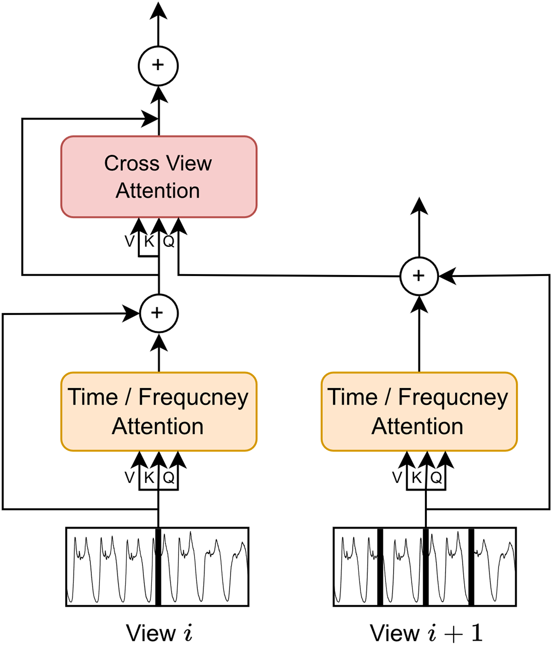
Figure 7: The structure of cross-view attention

4.3 View Encoder

After the sequence data is processed through the multi-view module as described above, we obtain the sequence data in different views. These segment sequences in different views vary in length. This sequence data, post embedding encoding processes, enters the attention-based encoder. Each view has a unique encoder. In this paper, we propose two different forms of attention layers: the temporal vanilla attention module, and the frequency enhanced attention module.

4.3.1 Temporal Vanilla Attention Module

The architecture diagram of this module is shown in Fig. 8. The attention block in the time domain utilizes the scaled dot-product attention method [20]. The input consists of queries and keys of dimension dk, and values of dimension dv. We choose the dot-product (multiplication) attention as our attention function. We compute the dot product of the query with all keys, divide each product by dk, and then apply the softmax function to obtain the weights of the values. We compute the attention function of a set of queries concurrently, bundling them into a matrix Q. The keys and values are also packed into matrices K and V. This allows us to compute the attention output matrix as:

Figure 8: The structure of temporal vanilla attention module

Attention(Q,K,V)=softmax(QKTdk)V(5)

4.3.2 Frequency Enhancement Attention Module

The structure of this module is shown in Fig. 9. The attention block in the frequency domain is generally inspired by the Frequency Enhanced Block with Fourier Transform proposed by Zhou et al. [23]. The input data x∈RN×D will first undergo a Fourier transformation, converting time-domain data to frequency-domain data. The transformed frequency-domain data is represented by Q∈CN×D. Then, for each frequency domain sequence, we retain only the first half. The aim of this operation is to reduce the occurrence of overfitting during training. The operation is represented by the following equation:

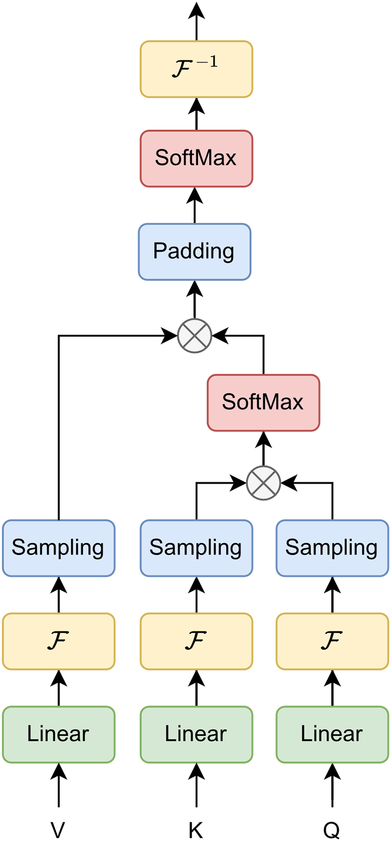
Figure 9: The structure of frequency enhancement attention module

Q~=Select(Q)=Select(ℱ(q))(6)

In this case, Q~∈C12N×D represents the retained frequency-domain sequence data. The attention block in the frequency domain can be defined as:

FEA(x)=ℱ−1(Padding(Q~⊙R))(7)

where R∈CD×D×12N is a learnable parameter. Let Y=Q⊙C, with Y∈C12N×D. The production operator ⊙ is defined as:

Ym,do=∑di=0DQm,di⋅Rdi,do,m(8)

where di=1,2,…,D denotes the input channel and do=1,2,…,D denotes the output channel. The result of Q~⊙R is then zero-padding to CN×D before performing inverse Fourier transform back to the time domain.

4.4 Global Encoder and Decoder

After the multi-view encoding is completed, data from each view, {s(i)}i=1V, will be integrated and entered into a linear transformation layer for dimension unification. Then, these data are sent into a global encoder, following Vaswani et al. [20]. The global encoder uses multiple Transformer layers to integrate the temporal trend information under different views. After data integration, it enters a global frequency-enhanced decoder for processing. Finally, the model outputs the final time series prediction results.

5  Experimental Section

5.1 Experimental Setup

5.1.1 Dataset

To evaluate the performance of our proposed model, we conducted a series of experiments. The base station signaling dataset we used has been described in detail in Section 3. After obtaining the preprocessed data, we standardized the dataset and divided it into training, validation, and test sets in chronological order, with a ratio of 7:1:2. Both the validation and test sets cover at least one full week, including weekdays and holidays.

5.1.2 Hyperparameter Settings

In this study, we set the time span of the input data to be 24 h. Due to the 5-min interval of the input data, the length of the input time series is 288. Simultaneously, we set each experimental model to predict the changes in the number of people over the next 24 h, so the length of the output prediction series is also 288. We evaluate the performance of different models by comparing the output prediction series with the actual series. In the experiments with the Transformer baseline model, to ensure fairness in model comparisons, we uniformly set the number of attention layers in the encoder to 2 and in the decoder to 1. We selected the mean squared error as the loss function and used the Adam optimizer for deep model training. The batch size and learning rate during training were set to 64 and 0.0001, respectively.

5.1.3 Performance Evaluation Metrics

We chose Mean Absolute Error (MAE), Mean Squared Error (MSE), Mean Absolute Percentage Error (MAPE), and Root Mean Squared Error (RMSE) as the metrics for evaluating model accuracy. Their definitions are as follows:

MAE=1n∑i=1n|y^i−yi|(9)

MSE=1n∑i=1n(y^i−yi)2(10)

MAPE=1n∑i=1n|y^i−yiyi|(11)

RMSE=1n∑i=1n(y^i−yi)2(12)

Firstly, we selected Mean Absolute Error (MAE) and Mean Squared Error (MSE) as evaluation metrics. We chose these metrics because they are commonly used for regression tasks and widely applied in various prediction problems, including population forecasting. MAE measures the average absolute difference between predicted values and true values, while MSE considers the square of the errors, thereby assigning higher penalties to larger errors. Since our task involves population prediction based on regression models, these metrics provide intuitive measures of error to help assess the accuracy and performance of our models.

Secondly, we included Mean Absolute Percentage Error (MAPE) as one of the evaluation metrics. This metric offers a relative measure of error, helping us understand the average percentage difference between the model's predictions and the true values. In population forecasting tasks, measuring relative error allows us to evaluate the model's performance across different scales, which is easier to comprehend and explain for decision-makers.

Finally, we chose Root Mean Squared Error (RMSE) as another evaluation metric widely used in regression tasks. RMSE provides the standard deviation of prediction errors by taking the square root of the mean of squared errors. This metric is useful in assessing the predictive performance and error magnitude of the models, particularly when comparing mean squared errors.

In summary, we selected these evaluation metrics to comprehensively consider different aspects of model performance and assess the accuracy and effectiveness of the proposed approach.

5.1.4 Baseline Models

We selected four Transformer-based models for comparison, namely Informer [33], Reformer [34], Autoformer [22], and FEDformer [23], as baseline models to evaluate the performance of our MVformer model.

Informer [33]. The Informer is an improved model built upon the Transformer, with the primary goal of enhancing model performance while reducing time complexity.

Reformer [34]. The Reformer is a memory-efficient and faster alternative to standard Transformer models, achieved through the use of reversible layers, locality-sensitive hashing attention, and other techniques.

Autoformer [22]. The Autoformer adds a decomposition block to extract the inherent complex temporal trends of the hidden states in the model, built on the design foundation of the Transformer framework.

FEDformer [23]. The FEDformer is a model proposed based on the Autoformer architecture. It applies attention mechanisms in the frequency domain and projects the time series signal into the frequency domain using the Fourier transform.

5.2 Results Analysis

To compare the performance of various models in long-term time series prediction tasks, and their behavior under different input and output lengths, we designed four sets of experiments, setting the input and output lengths to 144 and 288, respectively. Specifically, we input historical data spanning one and two days, and output long-term time series predictions spanning one and two days. In the context of our proposed MVformer, we conducted experiments separately using both temporal attention module (MVformer-t) and frequency enhancement attention module (MVformer-f).

5.2.1 Univariate Results

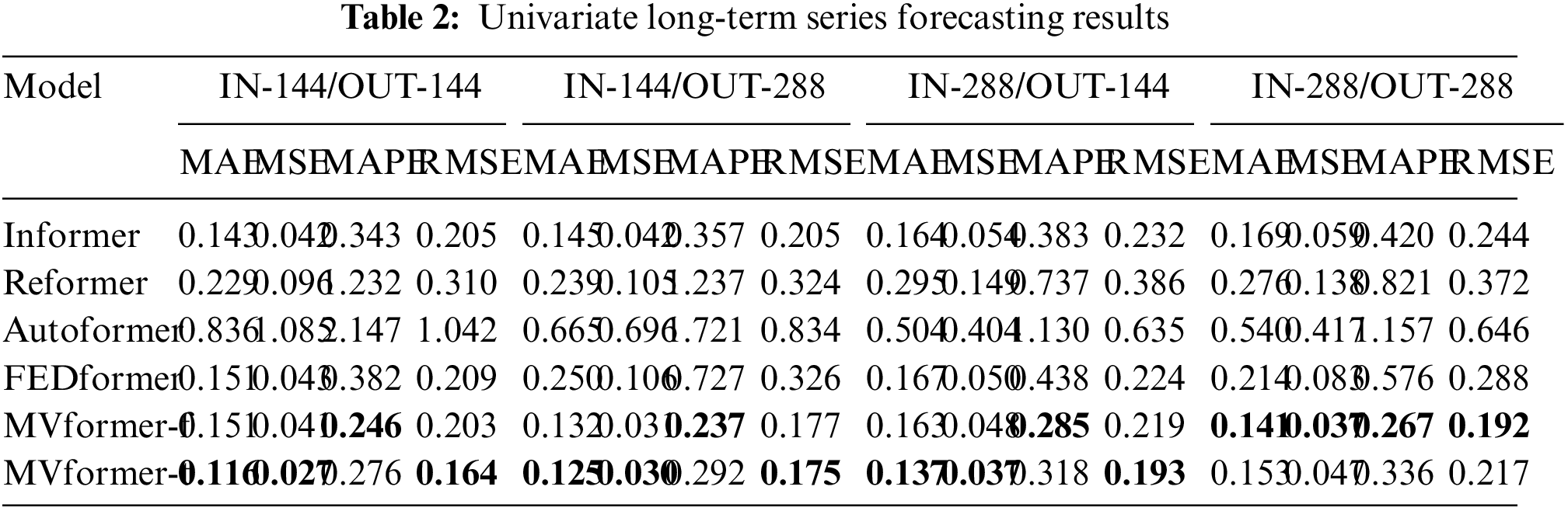
The univariate time series prediction results are presented in Table 2. Compared to FEDformer, MVformer achieved an average reduction of 34.7% in MSE. In the prediction task with an input history length of 144 and an output prediction length of 288, the improvement can even exceed 50%. It is worth noting that due to the differences in the temporal and frequency domain transformation modules, MVformer-f and MVformer-t exhibit different performances in different types of prediction tasks, complementing each other. This indicates the advantage of MVformer in long-term univariate time series prediction on the dataset used in this study.

To provide a comprehensive view of these various models on the population count time-series prediction task using our proposed dataset, we visualized both the predicted and actual data from the models. We plotted the whole predicted outcomes and corresponding ground truth from the univariate test data set in Fig. 10. Additionally, we plotted the single prediction data and corresponding ground truth data for various models where both the input and output sequence lengths are 288, as illustrated in Fig. 11. As evident from the graph, the MVformer model we proposed, whether based on the time-domain or frequency-domain method, successfully captures the cyclical changes in population density. Baseline models such as Autoformer diverge from the peaks and troughs of the ground truth curve, yet our MVformer model still accurately predicts the ground truth curve’s peaks and troughs. Compared to other models, our proposed MVformer is superior.

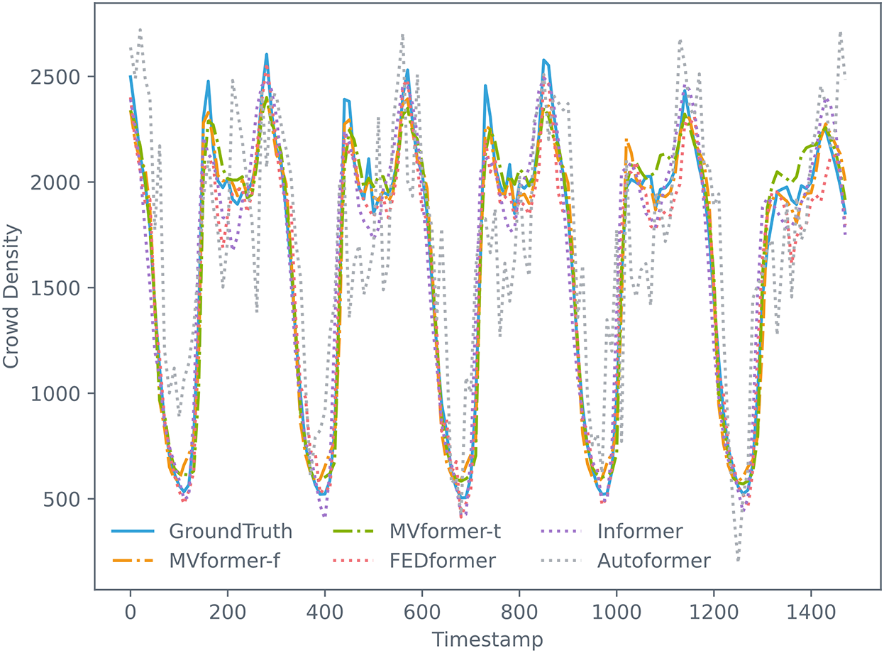
Figure 10: The prediction results of our proposed MVformer and baseline models during a period time

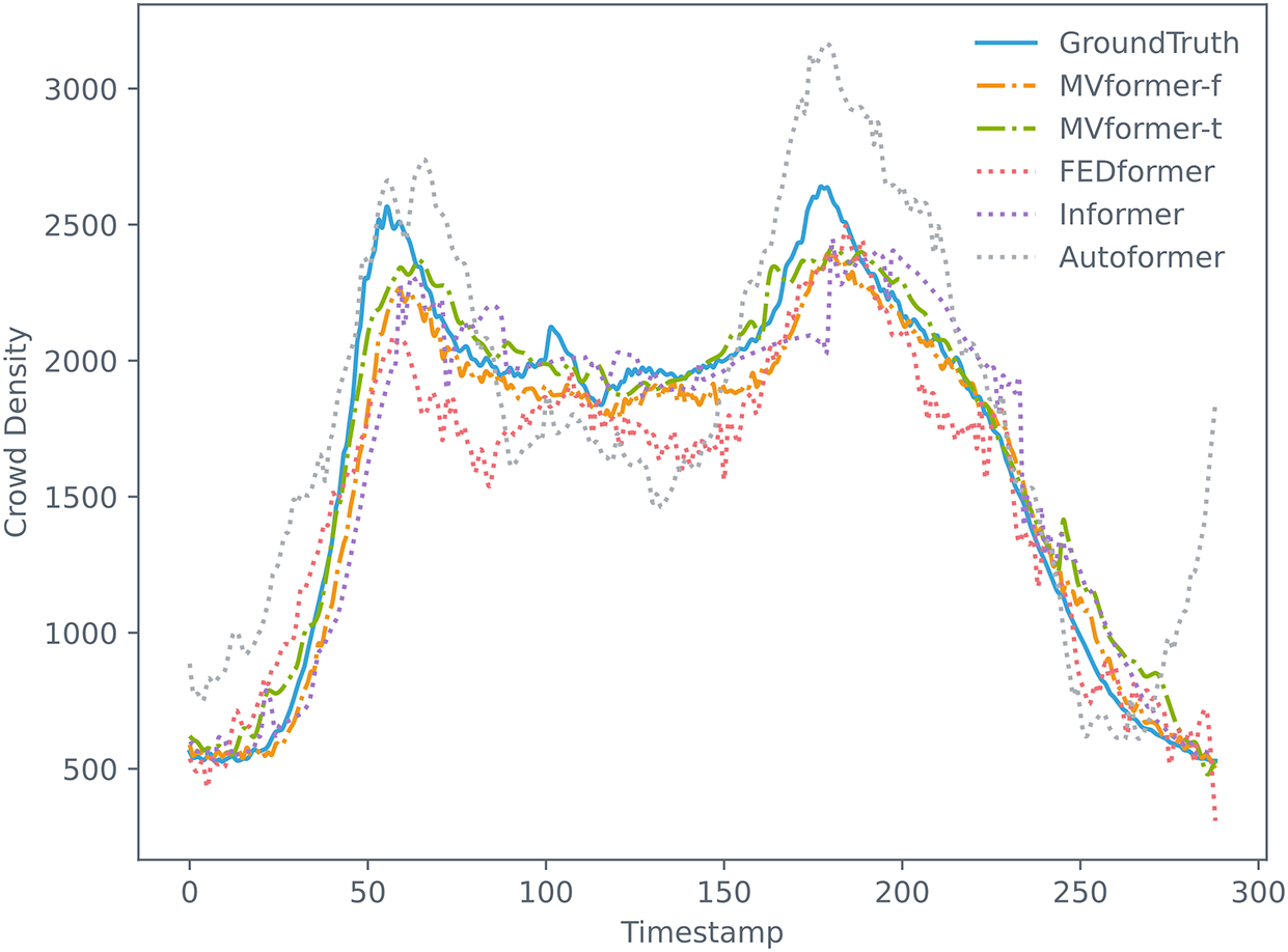
Figure 11: The results of our proposed MVformer and baseline models in a single prediction

5.2.2 Multivariate Results

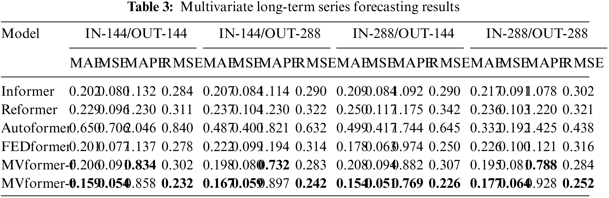
We conducted experiments on our multivariate dataset that includes population variations in all regions to evaluate the performance of our proposed MVformer in multivariate time series prediction. The experimental results are shown in Table 3. Compared to FEDformer, MVformer-t achieved an average reduction of 31.3% in MSE. In terms of the MSE metric, the MVformer-t model demonstrated the best performance across various types of prediction tasks. This highlights the advantage of MVformer in long-term multivariate time series prediction on the dataset used in this study.

The results presented above illustrate a comparison of various models on a multivariate population density dataset. Changes in population numbers exhibit a certain periodicity, which impacts the performance of the models in population count forecasting tasks. To investigate the spatial distribution of forecast errors in different regions, we calculated the average error based on the prediction data and actual data from different areas in the multivariate population dataset. We visualized the MAE and MAPE metrics as line graphs, as shown in Fig. 12. As can be seen from the figure, the model we proposed achieved the lowest MAE and MAPE values in most regions of this population count dataset. This suggests that our proposed model can adapt to various regions, achieving better long-term prediction performance in areas with strong population dynamics, and thereby yielding improved overall performance.

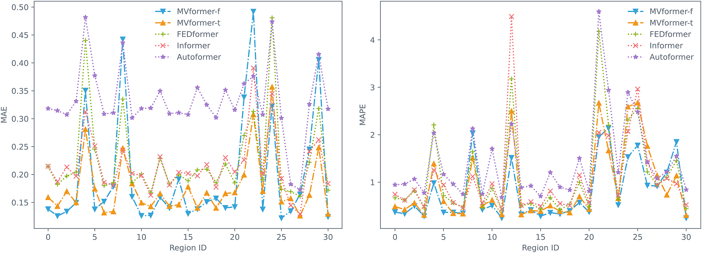
Figure 12: Prediction MAE (left) and MAPE (right) of every region

5.3 Ablation Study

In this study, we conduct an ablation study on the temporal dataset of the population of cellular base stations mentioned earlier, to explore the impact of different modules on the overall performance and prediction results of the MVformer model.

5.3.1 Model-View Assignments

In this study, the size of the view refers to the size of the sequence fragment. A larger view corresponds to larger subsequence fragments, which means fewer Transformer tokens. Conversely, a smaller view corresponds to smaller subsequence fragments, which means more Transformer tokens. Therefore, in the ablation experiments, we fixed the population size and the length of the input and output time series to be 288, and only considered a single view. By changing the size of the view, we examined the impact of the size of the individual view on the prediction results. We conducted three experiments with different view sizes, with the number of view fragments being 16, 72, and 144, respectively. The experimental results are shown in Table 4.

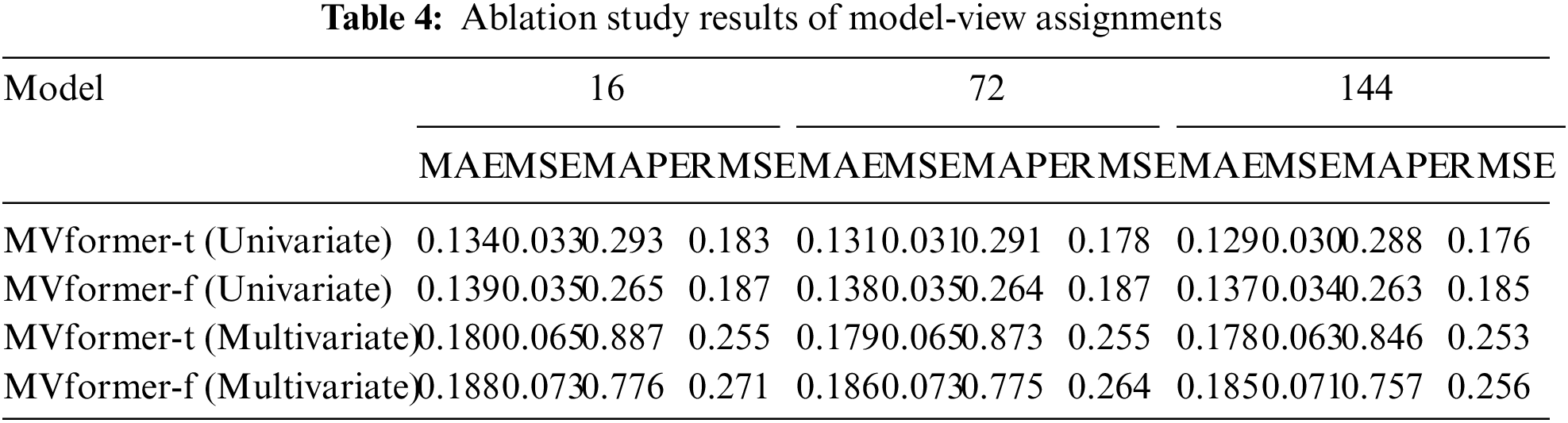
From the experimental results, it can be observed that as the size of the view decreases, the corresponding Transformer tokens increase, resulting in better predictive performance of the model. We interpret this as follows: in the case of a single view, a greater number of view tokens allows the model to learn more variations in the sequence. Consequently, the model can better fit and predict subsequent time series.

5.3.2 Effect of the Number of Views

To validate the impact of the number of views in the multi-view module on prediction results, we conducted three sets of experiments with varying numbers of views while keeping the population size and time series length of input and output fixed at 288. In the first set, we employed two segmentation strategies for the views (with 1 and 16 segments). In the second set, we used three segmentation strategies (with 1, 16, and 72 segments). In the third set, we utilized four segmentation strategies (with 1, 16, 72, and 144 segments). By conducting these three sets of experiments, we aim to investigate the influence of different numbers of views on the prediction results of the multi-view module regarding population size. The experimental results for this section are shown in Table 5.

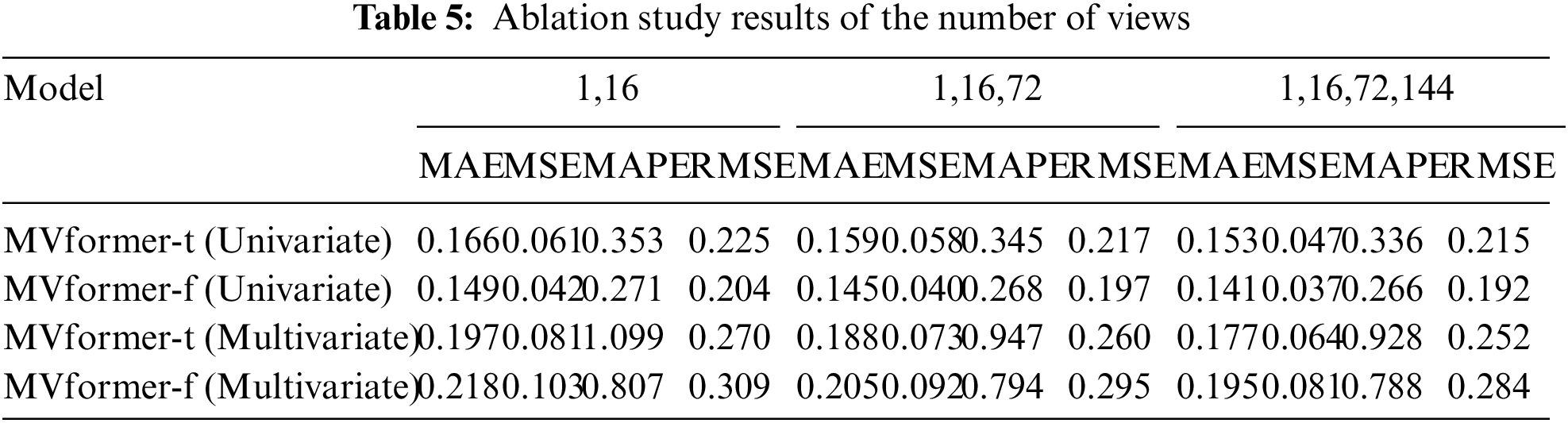
From the experimental results, it can be observed that the predictive performance of the model increases with the number of views. One possible explanation for this observation is that by increasing the number of views, the model could learn the pattern variations of the temporal sequence from different perspectives. As a result, the model can enhance the accuracy of temporal prediction through the multi-view module.

6  Conclusion

This paper presents a comprehensive method for preprocessing base station data, which handles temporal and spatial information, providing a reliable data foundation for predicting population quantities. Furthermore, a Transformer-based multi-view enhancement model, MVformer, is proposed to improve the accuracy of long-term population forecasting by incorporating Transformer structures and frequency domain enhancement techniques. Experimental results demonstrate the exceptional performance of our proposed model in population prediction tasks. To further enhance the accuracy and reliability of population density forecasting, future research could focus on refining existing models. This may involve incorporating additional data sources, exploring different network architectures, or developing hybrid models that combine multiple techniques. Moreover, future studies can further explore other application areas of base station data, improve the performance of prediction models, and strengthen research on model interpretability to enhance the accuracy and credibility of prediction results. Through continuous and in-depth research, we believe that the value of base station data can be better exploited and applied. In summary, continuous exploration and research on base station data, along with improvements in prediction models and interpretability, will maximize the value and applicability of this data source. As researchers delve deeper into these areas, the potential applications of base station data in smart cities will be fully realized, influencing critical areas such as urban planning, transportation management, industry applications, and public safety.

Acknowledgement: The authors would like to express their gratitude for the valuable feedback and suggestions provided by all the anonymous reviewers and the editorial team.

Funding Statement: This work was supported in part by Guangdong Basic and Applied Basic Research Foundation under Grant No. 2024A1515012485 and in part by the Shenzhen Fundamental Research Program under Grant JCYJ20220810112354002.

Author Contributions: Conceptualization, Yu Zhou and Bosong Lin; Data curation, Dandan Yu; Formal analysis, Siqi Hu and Dandan Yu; Investigation, Siqi Hu; Methodology, Yu Zhou, Bosong Lin and Siqi Hu; Validation, Bosong Lin and Siqi Hu; Visualization, Dandan Yu; Writing original draft, Yu Zhou and Bosong Lin. All authors reviewed the results and approved the final version of the manuscript.

Availability of Data and Materials: Data is available upon request.

Conflicts of Interest: The authors declare that they have no conflicts of interest to report regarding the present study.

References

1. S. Kumar, S. Indu, and G. S. Walia, “Smartphone traffic analysis: A contemporary survey of the state-of-the-art,” in Proc. ICMC, Dec. 2021, pp. 325–343. [Google Scholar]

2. Z. Huang et al., “Modeling real-time human mobility based on mobile phone and transportation data fusion,” Transp. Res. Part C Emerg. Technol., vol. 96, pp. 251–269, Nov. 2018. doi: 10.1016/j.trc.2018.09.016. [Google Scholar] [CrossRef]

3. Y. Liu, F. Fang, and Y. Jing, “How urban land use influences commuting flows in Wuhan, Central China: A mobile phone signaling data perspective,” Sustain Cities Soc, vol. 53, pp. 101914, Feb. 2020. doi: 10.1016/j.scs.2019.101914. [Google Scholar] [CrossRef]

4. K. Chin, H. Huang, C. Horn, I. Kasanicky, and R. Weibel, “Inferring fine-grained transport modes from mobile phone cellular signaling data,” Comput. Environ. Urban Syst., vol. 77, pp. 101348, Sep. 2019. doi: 10.1016/j.compenvurbsys.2019.101348. [Google Scholar] [CrossRef]

5. F. Calabrese, M. Diao, G. di Lorenzo, J. Ferreira Jr and C. Ratti, “Understanding individual mobility patterns from urban sensing data: A mobile phone trace example,” Transp. Res. Part C Emerg. Technol., vol. 26, pp. 301–313, Jan. 2013. doi: 10.1016/j.trc.2012.09.009. [Google Scholar] [CrossRef]

6. G. Zhong, T. Yin, J. Zhang, S. He, and B. Ran, “Characteristics analysis for travel behavior of transportation hub passengers using mobile phone data,” Transp., vol. 46, pp. 1713–1736, Oct. 2019. doi: 10.1007/s11116-018-9876-5. [Google Scholar] [CrossRef]

7. J. Huo, X. Fu, Z. Liu, and Q. Zhang, “Short-term estimation and prediction of pedestrian density in urban hot spots based on mobile phone data,” IEEE Trans. Intell. Transp. Syst., vol. 23, no. 8, pp. 10827–10838, Jul. 2021. doi: 10.1109/TITS.2021.3096274. [Google Scholar] [CrossRef]

8. P. Dai, S. Han, X. Yang, H. Fu, Y. Wang and J. Liu, “Analysis of the factors affecting the construction of subway stations in residential areas,” Sustainability, vol. 14, no. 20, pp. 13075, Oct. 2022. doi: 10.3390/su142013075. [Google Scholar] [CrossRef]

9. Y. Zheng, L. Capra, O. Wolfson, and H. Yang, “Urban computing: Concepts, methodologies, and applications,” ACM Trans. Intell. Syst. Technol., vol. 5, no. 3, pp. 1–55, Sep. 2014. doi: 10.1145/2629592. [Google Scholar] [CrossRef]

10. E. Chen, Z. Ye, C. Wang, and M. Xu, “Subway passenger flow prediction for special events using smart card data,” IEEE Trans. Intell. Transp. Syst., vol. 21, no. 3, pp. 1109–1120, May 2019. doi: 10.1109/TITS.2019.2902405. [Google Scholar] [CrossRef]

11. B. Yu, H. Yin, and Z. Zhu, “Spatio-temporal graph convolutional networks: A deep learning framework for traffic forecasting,” Jul. 2017. doi: 10.48550/arXiv.1709.04875. [Google Scholar] [CrossRef]

12. M. Heiskala, J. P. Jokinen, and M. Tinnilä, “Crowdsensing-based transportation services—An analysis from business model and sustainability viewpoints,” Res. Transp. Bus. Manag., vol. 18, pp. 38–48, Mar. 2016. doi: 10.1016/j.rtbm.2016.03.006. [Google Scholar] [CrossRef]

13. Z. Li et al., “Trip purposes mining from mobile signaling data,” IEEE Trans. Intell. Transp. Syst., vol. 23, no. 8, pp. 13190–13202, Oct. 2021. doi: 10.1109/TITS.2021.3121551. [Google Scholar] [CrossRef]

14. Q. Zhu and L. Sun, “Big data driven anomaly detection for cellular networks,” IEEE Access, vol. 8, pp. 31398–31408, Feb. 2020. doi: 10.1109/ACCESS.2020.2973214. [Google Scholar] [CrossRef]

15. S. Siami-Namini, N. Tavakoli, and A. S. Namin, “A comparison of ARIMA and LSTM in forecasting time series,” in Proc. ICMLA, Orlando, FL, USA, Dec. 2018. [Google Scholar]

16. J. Chung, C. Gulcehre, K. Cho, and Y. Bengio, “Empirical evaluation of gated recurrent neural networks on sequence modeling,” Dec. 2014. doi: 10.48550/arXiv.1412.3555. [Google Scholar] [CrossRef]

17. X. Zhang, F. Shen, J. Zhao, and G. Yang, “Time series forecasting using GRU neural network with multi-lag after decomposition,” in Proc. ICONIP, Oct. 2017, pp. 523–532. [Google Scholar]

18. I. Koprinska, D. Wu, and Z. Wang, “Convolutional neural networks for energy time series forecasting,” in Proc. IJCNN, Jul. 2018, pp. 1–8. [Google Scholar]

19. S. Bai, J. Z. Kolter, and V. Koltun, “An empirical evaluation of generic convolutional and recurrent networks for sequence modeling,” Apr. 2018. doi: 10.48550/arXiv.1803.01271. [Google Scholar] [CrossRef]

20. A. Vaswani et al., “Attention is all you need,” in Proc. NIPS, 2017. [Google Scholar]

21. S. Li et al., “Enhancing the locality and breaking the memory bottleneck of transformer on time series forecasting,” in Proc. NeurIPS, 2019. [Google Scholar]

22. H. Wu, J. Xu, J. Wang, and M. Long, “Autoformer: Decomposition transformers with auto-correlation for long-term series forecasting,” in Proc. NeurIPS, 2021, pp. 22419–22430. [Google Scholar]

23. T. Zhou, Z. Ma, Q. Wen, X. Wang, L. Sun, and R. Jin, “FEDformer: Frequency enhanced decomposed transformer for long-term series forecasting,” in Proc. PMLR, 2022, pp. 27268–27286. [Google Scholar]

24. X. Fu, G. Yu, and Z. Liu, “Spatial-temporal convolutional model for urban crowd density prediction based on mobile-phone signaling data,” IEEE Trans. Intell. Transp. Syst., vol. 23, no. 9, pp. 14661–14673, Sep. 2021. doi: 10.1109/TITS.2021.3131337. [Google Scholar] [CrossRef]

25. S. L. Ho and M. Xie, “The use of ARIMA models for reliability forecasting and analysis,” Comput. Ind. Eng., vol. 35, no. 1–2, pp. 213–216, Oct. 1998. doi: 10.1016/S0360-8352(98)00066-7. [Google Scholar] [CrossRef]

26. C. Bergmeir, R. J. Hyndman, and B. Koo, “A note on the validity of cross-validation for evaluating autoregressive time series prediction,” Comput. Stat. Data. Anal., vol. 120, no. 12, pp. 70–83, Apr. 2018. doi: 10.1016/j.csda.2017.11.003. [Google Scholar] [CrossRef]

27. S. S. Roy, D. Mittal, A. Basu, and A. Abraham, “Stock market forecasting using LASSO linear regression model,” in Afr-Eur. Conf. Ind. Adv., 2015, pp. 371–381. [Google Scholar]

28. R. Yadav, W. Zhang, O. Kaiwartya, H. Song, and S. Yu, “Energy-latency tradeoff for dynamic computation offloading in vehicular fog computing,” IEEE Trans. Veh. Technol., vol. 69, no. 12, pp. 14198–14211, Dec. 2020. doi: 10.1109/TVT.2020.3040596. [Google Scholar] [CrossRef]

29. W. Jiang and J. Luo, “Graph neural network for traffic forecasting: A survey,” Expert Syst. Appl., vol. 207, no. 7, pp. 117921, Nov. 2022. doi: 10.1016/j.eswa.2022.117921. [Google Scholar] [CrossRef]

30. W. Jiang, J. Luo, M. He, and W. Gu, “Graph neural network for traffic forecasting: The research progress,” ISPRS Int. J. Geo-Inf., vol. 12, no. 3, pp. 100, Feb. 2023. doi: 10.3390/ijgi12030100. [Google Scholar] [CrossRef]

31. C. Ling et al., “An edge server placement algorithm based on graph convolution network,” IEEE Trans. Veh. Technol., vol. 72, no. 4, pp. 5224–5239, Apr. 2022. doi: 10.1109/TVT.2022.3226681. [Google Scholar] [CrossRef]

32. M. Ay, S. Kulluk, L. Özbakır, B. Gülmez, G. Öztürk and S. Özer, “CNN-LSTM and clustering-based spatial-temporal demand forecasting for on-demand ride services,” Neural. Comput. Appl., vol. 34, no. 24, pp. 1–16, Aug. 2022. doi: 10.1007/s00521-022-07681-9. [Google Scholar] [CrossRef]

33. H. Zhou et al., “Informer: Beyond efficient transformer for long sequence time-series forecasting,” in Proc. AAAI, May 2021, pp. 11106–11115. [Google Scholar]

34. N. Kitaev, U. Kaiser and A. Levskaya, “Reformer: The efficient transformer,” Feb. 2020. doi: 10.48550/arXiv.2001.04451. [Google Scholar] [CrossRef]