CHART: Intelligent Crime Hotspot Detection and Real-Time Tracking Using Machine Learning

1  Introduction

Crime is an act that violate the laws of a society, typically leading to prosecution and punishment by the state [1]. These acts range from minor infractions, such as petty theft and vandalism, to severe offenses like murder and terrorism. The effects of crime are profound and multifaceted, impacting individuals, communities, and society at large [2]. On an individual level, victims of crime can suffer physical harm, psychological trauma, and financial loss, which can lead to long-term emotional distress and a diminished quality of life [3]. Communities affected by high crime rates often experience a breakdown of social cohesion and trust, leading to fear, decreased property values, and economic decline. Businesses may be reluctant to invest in high-crime areas, exacerbating unemployment and poverty. Societally, crime strains public resources, including law enforcement, judicial systems, and correctional facilities. It also necessitates substantial government expenditure on policing, legal proceedings, and incarceration [4]. Moreover, pervasive crime can erode public confidence in the rule of law and governance, leading to broader social stability and development implications. Thus, understanding and addressing crime is essential for promoting safety, justice, and prosperity within any community [5].

A crime hotspot is a specific geographic area where the frequency of criminal activity is significantly higher compared to other areas. These hotspots often cluster crimes, such as theft, assault, or vandalism, making them focal points for law enforcement and community safety efforts [6]. Identifying and understanding crime hotspots is crucial for effective policing, as it allows for strategically deploying resources, targeted patrols, and proactive crime prevention measures. Hotspot detection is the process of identifying these high-crime areas using various analytical techniques and data sources. This process involves collecting and analyzing crime data, often including details such as the type of crime, location, time of occurrence, and other relevant factors. Advanced methods, such as statistical analysis, Geographic Information Systems (GIS), and machine learning algorithms like Kernel Density Estimation (KDE) are used to visualize and predict hotspots [7]. These tools help in mapping out the intensity and distribution of criminal activities, enabling law enforcement agencies to focus their efforts on areas that need the most attention, thereby enhancing public safety and reducing crime rates.

Traditional hotspot detection methods have primarily involved manual analysis, statistical approaches, and basic Geographic Information Systems (GIS). Manual analysis entails law enforcement personnel reviewing crime reports and records to identify high-crime areas. This method often involves plotting incidents on physical maps or simple digital tools and visually identifying clusters of criminal activity [8]. While this approach can provide insights, it is labor-intensive and time-consuming. Additionally, it is highly susceptible to human error and subjective bias, which can lead to inconsistent and inaccurate hotspot identification. The manual process’s limitations make it difficult to keep up with the dynamic and evolving nature of criminal activity. Statistical methods, such as point pattern analysis and spatial autocorrelation, have also been used to detect crime hotspots [9]. These techniques involve calculating the density and distribution of crime incidents within a given area. Point pattern analysis focuses on identifying statistically significant clusters of events, while spatial autocorrelation measures the degree to which crime events are spatially correlated. Although these methods offer a more systematic approach than manual analysis, they are often limited by their reliance on predefined statistical models and thresholds, which may not accurately capture the complexities of real-world crime patterns.

Basic GIS-based methods have advanced traditional hotspot detection by enabling the visualization of crime data on digital maps. Tools like heat maps and thematic maps allow for a more intuitive understanding of crime distribution [10]. However, these methods still have significant limitations. Basic GIS tools often lack the analytical depth required to identify nuanced patterns and trends. They may not effectively integrate multiple data sources or consider the influence of various socio-economic and environmental factors on crime. Furthermore, these methods usually provide static representations of crime data, failing to capture criminal activity’s dynamic and temporal aspects.

Addressing these challenges may require a better model and practical implementation strategies to ensure that machine learning models provide reliable and actionable insights for crime prevention and law enforcement [11,12]. The proposed CHART represents a significant advancement over traditional and existing machine learning methods for crime hotspot detection. By integrating comprehensive data preprocessing, robust feature engineering, and sophisticated algorithms like Adaptive Synthetic Sampling (ADASYN) and Kernel Density Estimation (KDE), CHART effectively addresses the limitations of previous approaches, such as inefficiencies, biases, and computational complexity. The use of a Random Forest-based model ensures high accuracy and robustness, mitigating overfitting and enhancing generalizability. CHART’s ability to deliver precise, timely, and actionable insights into crime patterns significantly outperforms benchmark methods, allowing law enforcement agencies to allocate resources and improve crime prevention and response strategically. This framework sets a new standard for dynamic spatial analysis and prediction, providing a powerful tool for enhancing public safety and community well-being.

The key contribution of the proposed research are as follows:

•   Utilization of advanced feature engineering techniques using domain-specific knowledge, such as time of day, location type, and historical crime frequency, to extract and transform relevant features for improved model performance.

•   Introducing Kernel Density Estimation (KDE) for precise spatial analysis and visualization of crime hotspots, enabling effective resource allocation and strategic planning for law enforcement agencies.

•   Experimental results demonstrate that the CHART framework outperforms benchmark methods in crime hotspot detection, achieving higher accuracy, precision, recall, and F1 scores, thus providing more reliable and actionable insights for law enforcement agencies.

The rest of the paper is organized as follows: Section 2 reviews the current literature on hotspot detection techniques, Section 3 outlines the core methodology of the proposed work, Section 4 presents the experimental evaluations and results. Section 5 illustrates the application of CHART and Section 6 discusses the conclusion and directions for future work.

2  Literature Review

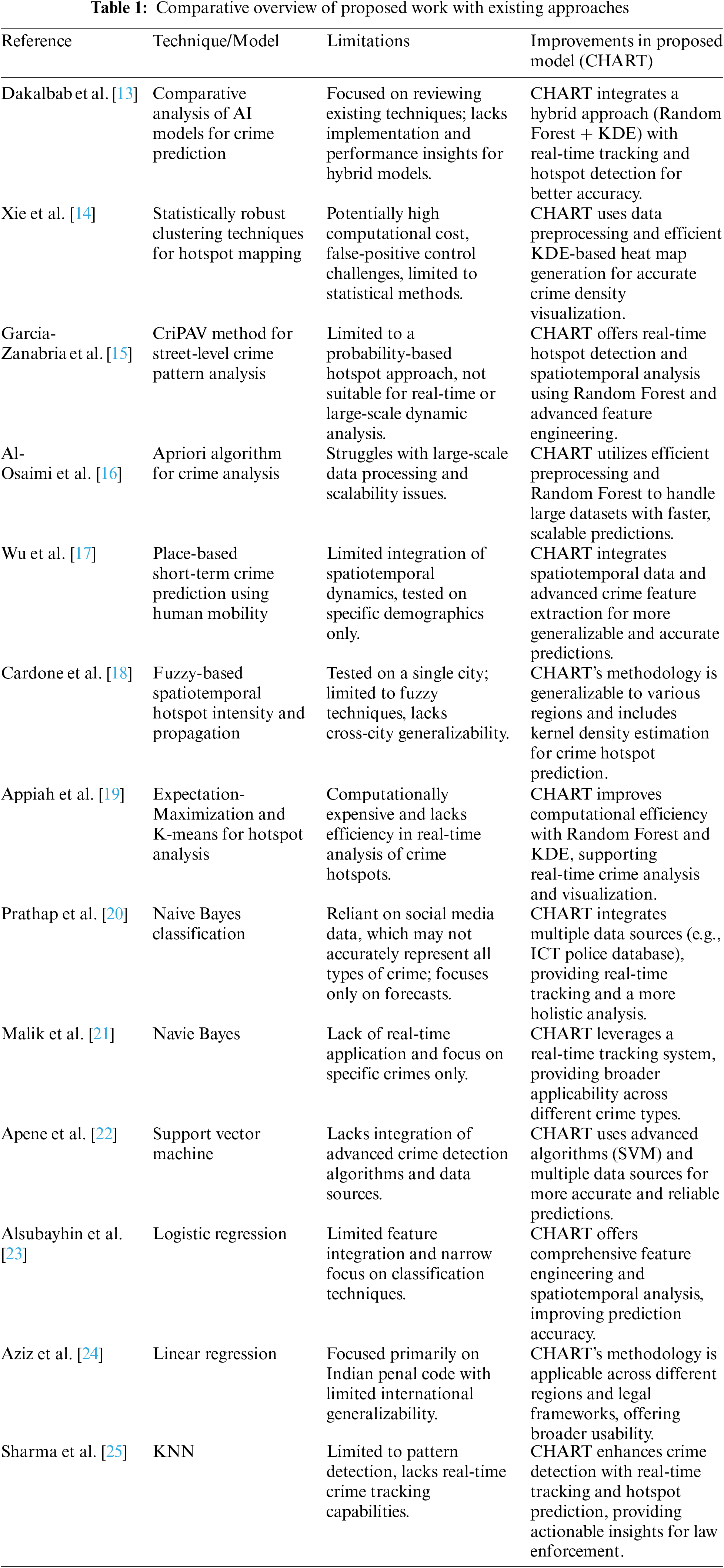
This section discusses the current literature that has been carried out in the domain of crime prediction. Dakalbab et al. [13] proposed a comparative analysis of different artificial intelligence based model to predict and prevent crime. The authors did a study where they reviewed 120 research papers about AI and crime prediction. They looked at the different types of crimes studied and the techniques used to predict them. They found that supervised learning was the most common approach used. They also looked at the strengths and weaknesses of the different techniques. They found that AI can be very effective in predicting crime, especially when used to identify crime hot spots. Hybrid models also showed promise. In the end, they suggested that more research should be done on hybrid models and that they plan to do further experiments to improve their own solution.

Xie et al. [14] discussed that spatial hotspot mapping is important in many areas like public health, public safety, transportation, and environmental science. It helps to identify areas with high rates of certain events like disease or crime, but traditional clustering techniques can give false results, which can be costly. To solve this problem, they developed a statistically robust clustering techniques, which use rigorous statistical methods to control false results. This article provides an optimized technique, including data modeling, region enumeration, maximization algorithms, and significance testing. The goal was to stimulate new ideas and approaches in computing research and help practitioners choose the best techniques for their needs. The work of Garcia-Zanabria et al. [15] discussed the challenges of understanding crime patterns in big cities. Crime is often spread out and hard to see, making it difficult and expensive to analyze. Their article introduced a new method called CriPAV, which helps experts analyze street-level crime patterns. CriPAV has two main parts: a way to find likely hotspots of crime based on probability, not just intensity, and a technique to identify similar hotspots by mapping them in a Cartesian space. CriPAV has been tested with real crime data in Sao Paulo and has been shown to help experts understand crime patterns and how they relate to the city.

Law enforcement authorities need to use data-driven strategies to prevent and detect crimes, as proposed by Al-Osaimi et al. [16]. However, their work limits the amount of data generated every day is increasing, which makes it difficult to process and store it. Their article also new Apriori algorithm to analyze crime by using various datasets. They designed a crime analysis tool for public safety and data mining that helps law enforcement officers to make better decisions. Wu et al. [17] proposed a place-based short-term crime prediction model that used patterns of past crimes to predict future crime incidents in specific locations. Their model was based on the concept human mobility that can contribute to limited crime generation. They used a large-scale human mobility dataset to evaluate the effects of human mobility features on short-term crime prediction. In addition to this, they also tested various neural network models on different cities with diverse demographics and types of crimes and found that adding human mobility flow features to historical crime data can improve prediction accuracy.

Cardone et al. [18] presented a fuzzy-based spatiotemporal hot spot intensity and propagation technique. Their work explained a new way to study “hot spots,” where a certain thing is happening a lot. The method involves using a computer program to find these hot spots and measure how strong they are. Their method was tested by looking at crime in the City of London over several years, and the results showed that crime has been decreasing in all parts of the city. Their method seems to be reliable and could be used in the future to study other things happening in different places. Appiah et al. [19] also discussed a model-based clustering of expectation maximization and K-means algorithms in crime hotspot analysis to fix crime in different areas. They used a mathematical method called Gaussian multivariate distributions to estimate potential crime hotspots. This involves finding the best way to group data points into clusters to identify areas where crimes are likely to occur. They used a large dataset of violent crimes and analyzed the data using a combination of K-means clustering and the expectation-maximization (E-M) algorithm. They found that this new method is efficient and fast and produced similar results to traditional methods.

Prathap et al. [20] discussed a geospatial crime analysis and forecasting with machine learning techniques paper. In their work, they discussed that people used social media to connect with others, share ideas and content, and for professional purposes. Researchers are able to analyze individual behavior and interactions on social media sites like Facebook and Twitter. Criminology is an area of study that uses data gathered from online social media to understand criminal activity better. Researchers can obtain valuable information about crime by analyzing user-generated content and spatiotemporal linkages. This research examines 68 crime keywords to categorize crime into subgroups based on geographical and temporal data. The proposed Naive Bayes-based classification algorithm is used to classify crimes, and the Mallet package is used to retrieve keywords from news feeds. Their study identifies crime hotspots using the K-means method and uses the KDE approach to address crime density. The study found that the suggested crime forecasting model is equivalent to the ARIMA model. The comparative overview of the proposed work with existing approaches is given in Table 1.

3  Research Methodology

This section discusses the core methodology of CHART, which is majorly composed of data collection, preprocessing, feature extraction, and prediction. The proposed methodology in Fig. 1 combines various data sources, including police reports, public databases, and social media, to create a comprehensive crime prediction model, CHART. It starts with a robust text preprocessing pipeline that cleans and prepares data by removing URLs, converting text to lowercase, removing numbers, joining text tokens, and stripping punctuation. This clean data is then subjected to feature extraction, where domain knowledge is applied to extract relevant crime-related attributes like time, location, and type. These features are ranked and labeled to prepare for machine learning analysis. The model uses Kernel Density Estimation (KDE) to generate a heat map, visually representing crime hotspots as smooth data point distributions. Finally, a Random Forest-based approach is employed for crime detection, utilizing decision trees that aggregate predictions through majority voting or averaging to identify potential crime hotspots effectively. This comprehensive approach aims to enhance real-time crime prediction and hotspot detection, providing law enforcement with actionable insights for targeted interventions.

Figure 1: Proposed model for crime analysis and hotpot detection

3.1 Data Collection

Three different dataset has been used for the evaluation of CHART. The first dataset used to train and test the model is sourced from Kaggle.com, accessed on 16 February 2024, specifically from the “Crime in Vancouver” dataset. This dataset comprises two files: Crime.csv and GoogleTrend.csv. The Crime.csv dataset contains 530,652 crime records spanning from 01 January 2006, to 13 July 2021, and includes ten features: type of crime, year, month, day, hour, minute, hundredth block, and neighborhood. The GoogleTrend.csv dataset includes 185 records with two features: search value and month-year. Overall, the Vancouver crime dataset covers 14 years of crime data, featuring various types of crimes such as Theft from a Vehicle and Break and Enter Residential/Other. The neighborhoods represented in the dataset include Fairview, Victoria-Fraserview, Strathcona, Downtown, Grandview-Woodland, Kensington-Cedar Cottage, West End, Oakridge, Killarney, and Sunset. The dataset description is shown in Table 2.

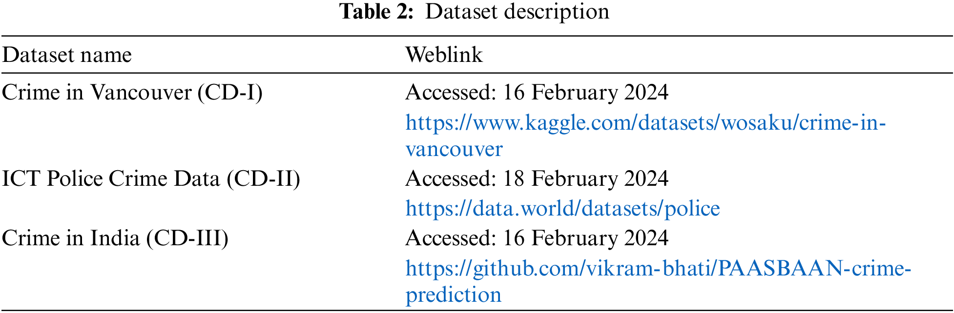
The very next dataset consists of four entries categorized by zones: City, Saddar, Industrial Area, and Rural and contains 120,442 crime records spanning from 2009, 2021. It is sourced from the ICT police database. The dataset likely contains information related to law enforcement activities within these zones, potentially including crime statistics, incident reports, and other relevant data. With this dataset, researchers and analysts can explore and analyze the patterns, trends, and characteristics of policing and security in different ICT regions. Each entry contains information such as a unique identifier (e.g., ICT-6/14/2023-2256), the name and contact number the person reporting the crime, zone, police station, crime nature, crime type, crime location, latitude longitude, offence of, the nature of the crime (e.g., Other Crime, Robbery, Begging Act), the date and time of the report, the duration of the incident, and the current status (e.g., Pending). The third dataset includes 530,652 records of crime incidents in India, which contains detailed information about each crime. It comprises of 10 features, including type of crime, year, month, day, hour, minute, hundredth block, and neighborhood, while the file includes 185 records with two features, namely search value and month-year.

3.2 Data Preprocessing

Data preprocessing is an important step in any data analysis and machine learning pipeline. It involves the preparation and transformation of raw data into a format suitable for analysis and model training. Proper preprocessing ensures that the data is clean, consistent, and free from errors, directly impacting machine learning models’ performance and accuracy. This step typically includes handling missing values, correcting inconsistencies, standardizing or normalizing features, and encoding categorical variables. Additionally, feature engineering may be applied to create new, more informative variables that enhance the predictive power of the model. By ensuring data quality and relevance, preprocessing sets the foundation for building effective machine learning models.

Algorithm 1 shows the preliminary data preprocessing, a key step in the data analysis and machine learning pipeline that transforms raw data into a clean and usable format. This process enhances data quality by correcting errors, handling missing values, and ensuring consistency across different sources. It also improves model performance by standardizing or normalizing features, removing irrelevant information, and encoding categorical variables while creating new features.

Additionally, data preprocessing simplifies analysis through visualization and summary statistics, enabling the identification of patterns and trends. It ensures robust and reliable results by reducing biases and improving the model’s ability to generalize to new data. Key steps in data preprocessing include data acquisition, which involves gathering raw data from various sources; data cleaning, where errors and inconsistencies are corrected, and missing values are handled; noise removal, which eliminates irrelevant or misleading information that could distort analysis; and normalization, where data is scaled to ensure uniformity across features. These steps work together to produce a consistent, accurate, and complete dataset, laying the groundwork for effective analysis or machine learning modeling.

3.3 Data Balancing

Data balancing is essential in machine learning, especially when dealing with imbalanced datasets, where one class of data significantly outnumbers another. It involves adjusting the distribution of data samples across different classes to ensure that the machine learning model learns from a representative set of examples from each class, thus improving its performance and generalization ability. One commonly used technique for data balancing is called “oversampling” or “undersampling,” which involves either increasing the number of samples in the minority class (oversampling) or reducing the number of samples in the majority class (undersampling). Here’s an algorithm and example code for data balancing using oversampling:

Adaptive Synthetic Sampling (ADASYN) has been adopted in this research, a powerful data balancing technique used to address class imbalance in datasets by generating synthetic samples for the minority class [26]. ADASYN focuses on developing synthetic samples for the minority class to balance the dataset, thereby improving the performance of machine learning models. The process begins by calculating the imbalance ratio τ between the minority class Cm and the majority class CM: τ=CmCM. Where Cm and CM are the number of samples in the minority and majority classes, respectively. ADASYN then determines the number of synthetic samples G to generate using Eq. (1).

G=(|CM|−|Cm|).β(1)

where β is a parameter that controls the desired level of balancing. For each minority class sample xi, ADASYN calculates the k-nearest neighbors Ni and computes the density distribution Δi as shown in Eq. (2).

Δi=δik(2)

pi=Δi∑i=1|Cm|Δi(3)

The number of synthetic samples gi to be generated for each minority sample xi is: gi=G.pi. New synthetic samples are created by interpolating between xi and its k-nearest neighbors. For each synthetic sample, a random neighbor xik is selected, and a new sample is generated using Eq. (4).

χ=xi+λ.(xik−xi)(4)

where λ is a random number in the range [0, 1], this approach ensures that more synthetic samples are generated for minority samples that are harder to learn, thereby enhancing the model’s ability to generalize across different classes. By integrating ADASYN into our preprocessing pipeline, we achieve a balanced dataset that significantly improves the robustness and accuracy of our crime detection models.

3.4 Feature Engineering

Feature engineering is a critical step in the machine learning pipeline, laying the groundwork for building effective and robust models. It involves a combination of domain knowledge, creativity, and algorithmic techniques to extract relevant information from raw data and present it in a format that best serves the learning task at hand. In this research, three different tasks, feature extraction, feature labeling, and feature ranking, were carried out to pick the most important features. The details of each phase are as follows.

3.4.1 Feature Extraction Process

Due to the sensitive nature of the data and its real-time application, the custom rules based on a domain knowledge-based feature extraction process have been adopted in this research. This involves creating features that leverage specific insights and patterns relevant to the domain of crime analysis. This process typically begins with an in-depth understanding of the domain, then identifying relevant attributes and transforming raw data into meaningful features. The first step involves collaborating with domain experts, such as criminologists or law enforcement officers, to gather insights into the patterns and characteristics of criminal activities. For instance, understanding the significance of crime types, locations, times, and demographic factors can provide a foundation for creating relevant features. Based on domain knowledge, identify attributes that are likely to influence crime patterns. Common attributes in crime data include:

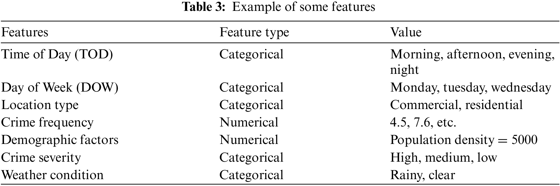
•   Time of Day (TOD): Crimes might follow daily patterns, with different types of crimes occurring at different times.

•   Day of Week (DOW): Weekdays and weekends can show different crime patterns.

•   Location Type: Different areas (residential, commercial, public spaces) might have distinct crime rates.

•   Demographic Factors: Age, gender, and socio-economic status of the population can impact crime rates.

Use domain knowledge to transform raw attributes into meaningful features. For instance, the Time of Day features encode the time of day into categorical variables (morning, afternoon, evening, night) or use sine and cosine transformations to capture cyclical patterns, as shown in Eqs. (5) and (6).

TODsin=sin⁡(2π.hours24)(5)

TODcos=cos⁡(2π.hours24)(6)

Similarly, for Day of Week, One-hot encode the day of the week to capture weekly patterns.

To create a composite feature, a combination of multiple attributes is applied to create composite features that capture more complex patterns. For example, for the Time and Location Interaction, crimes might have different patterns depending on both the time of day and the location. Create interaction terms to capture these effects as given in Eq. (7).

Time_Location_Interaction=TOD×Location_Type(7)

Similarly, for Crime Frequency by Area, it calculates the historical crime frequency for different areas to identify hotspots. Use a moving average to smooth out short-term fluctuations as shown in Eq. (8).

Crime.Frequencyarea=1N∑i=1NCrimesarea,i(8)

where N is the number of time periods considered.

3.4.2 Labeling and Ranking

For labeling each feature as a criminal nature, this work uses domain-specific information as described by law and order to label and categorize features. However, the categorize crime placed into low, medium, and high categories based on these information:

Crimecategory={LowifCrimefrequency<αMediumifCrimefrequency<βHighifCrimefrequency≥β(9)

where α and β are law and forcemeat agencies’ scores against each crime determined from the data. Once the features are created, they can be used to train machine learning models for crime detection and heat map generation. It’s crucial to evaluate the effectiveness of these features by comparing model performance with and without the custom rules-based features. Based on the labeling, the most important features, the top 10 features can be selected based on their importance scores by using:

I(f)=1N∑i=1NIt(f)(10)

where It(f) is the importance of feature f in t label and N is the total number of features. Examples of extracted features are given in Table 3.

3.5 Heat Map Generation

The process of generating a heat map, as shown in Fig. 2 for crime detection and analysis, involves multiple steps, starting with data collection and ending with visualization. The first step is to gather and preprocess the spatial data, such as crime incidents, ensuring that each data point has corresponding latitude and longitude coordinates. This involves cleaning the data to remove any inconsistencies or errors and formatting it appropriately for analysis. Accurate and clean data is crucial for reliable heat map generation. The next step involves selecting the kernel function and bandwidth for Kernel Density Estimation (KDE), a non-parametric way to estimate the probability density function of a random variable. KDE is particularly useful for visualizing the intensity of events over a geographical area. The Gaussian kernel is a common choice due to its smooth and continuous nature. The kernel function can be defined as:

K(u)=12πe−12u2(11)

Figure 2: Heat map snippet indicating top most crimes

The bandwidth, denoted as h, determines the level of smoothing applied to the data. It is a critical parameter as it affects the granularity of the resulting heat map. Bandwidth selection can be done using cross-validation or heuristic methods to balance between over-smoothing and under-smoothing the data.

Kernel Density Estimation is then used to calculate the density at each point on the map. The estimated density f′(x) at a point x is given by the equation:

f′(x)=1nh2∑i=1nK(x−xih)(12)

where n is the number of data points, xi are the data points, and K is the kernel function. This equation essentially sums up the contributions of each data point to the density estimate at x, weighted by their distance from x as determined by the kernel function and bandwidth.

After calculating the density estimates, a grid is created over the geographical area of interest. Each cell in this grid represents a point where the density is estimated. The density values at these grid points are computed using the KDE formula. These values are then used to visually represent the density, typically using a color scale where higher density values (indicating crime hotspots) are shown in warmer colors such as red, and lower density values are shown in cooler colors like blue. The generated heat map visually represents crime intensity across different areas, highlighting hotspots where criminal activities are concentrated. This visualization is useful for law enforcement agencies to allocate resources more effectively, plan patrols, and implement preventive measures in high-risk areas. By adjusting the bandwidth, the smoothness of the heat map can be fine-tuned to achieve the desired resolution, balancing between too-coarse and too-detailed visualizations.

3.6 Crime Prediction

The final step in the crime detection model involves identifying crime hotspots using a Random Forest-based model. This method leverages the ensemble learning approach, where multiple decision trees are constructed during training. Each decision tree is trained on a subset of the data, and their predictions are aggregated to improve overall accuracy and robustness. This approach mitigates overfitting, a common problem in individual decision trees, by averaging the predictions of multiple trees.

The Heat Map Generation step, which utilizes Kernel Density Estimation (KDE), primarily focuses on creating visual representations of crime density. This step highlights areas where crime incidents are concentrated based on historical data, giving law enforcement a geographical view of hotspots. On the other hand, the Random Forest prediction step is responsible for predicting future crime occurrences. It takes a broader set of features, such as time, location, crime type, and demographic factors, to predict the likelihood of future crimes and identify potential new hotspots that may not be visible from historical data alone. These two processes complement each other but serve different purposes: KDE provides a spatial visualization of existing crime hotspots, while Random Forest offers predictive insights by analyzing multiple factors, enabling law enforcement to anticipate future crime hotspots. We have made these distinctions clearer in the manuscript to improve understanding of how both steps contribute to the overall crime detection framework.

The choice of Random Forest in the CHART framework is motivated by several key attributes that make it particularly suitable for crime hotspot detection. First, the ability of Random Forest to handle large datasets with numerous predictors is essential, as crime data often involves complex interactions among various socio-demographic and spatial factors. Random Forest effectively captures these interactions without the need for extensive data transformation that other models might require. Second, the algorithm provides an inherent feature importance measure, which is invaluable for understanding the driving forces behind crime patterns. This aspect is crucial for not only predicting where crimes are likely to occur but also for developing informed strategies to mitigate these risks. Lastly, Random Forest’s ensemble approach, which builds multiple decision trees and aggregates their results, offers a reduction in variance and improves generalization over single predictive models. This approach minimizes overfitting—a common problem in predictive modeling of crime data where the model performs well on training data but poorly on unseen data. The robustness provided by Random Forest is advantageous in ensuring reliable predictions that are critical for deploying law enforcement resources effectively.

The Random Forest algorithm begins by randomly sampling the dataset with replacement, a process known as bootstrapping. For each tree in the forest, a different subset of the data is used for training. This introduces diversity among the trees, as each tree may see a slightly different dataset. Additionally, at each split in a tree, only a random subset of features is considered for splitting. This randomness further ensures that the trees are decorrelated, making the ensemble’s aggregated prediction more reliable.

y′=1N∑i=1NTt(x)(13)

where y′ is the predicted output, NNN is the number of trees in the forest, and Ti(x) is the prediction of the i-th tree for input x. By aggregating the predictions, usually through majority voting for classification tasks or averaging for regression tasks, the Random Forest model produces a more accurate and stable prediction compared to individual decision trees. The preprocessed and balanced dataset serves as the training ground for the Random Forest model. Important features, such as time of day, location type, and historical crime frequency, are used as inputs. These features are derived from earlier steps in the methodology, including data collection, preprocessing, and feature engineering. By incorporating domain knowledge and ensuring a balanced dataset, the model is better equipped to learn the complex patterns associated with crime incidents.

Once trained, the Random Forest model can predict the likelihood of crime incidents in different areas, effectively identifying hotspots. These predictions can be visualized on a map, where areas with higher predicted crime rates are marked as hotspots. This spatial representation allows law enforcement agencies to focus their resources on areas that are more prone to criminal activities, enhancing their ability to prevent and respond to crimes. The effectiveness of the Random Forest-based hotspot detection is evaluated using various metrics, such as accuracy, precision, recall, and F1-score. By comparing the model’s performance on a validation set, the parameters and structure of the Random Forest can be fine-tuned to achieve optimal results. This iterative process ensures that the model remains robust and accurate, providing valuable insights into crime patterns and aiding in the development of targeted crime prevention strategies.

The Random Forest algorithm, central to our CHART framework, is designed to handle complex datasets with multiple interacting features. It operates by constructing a collection of decision trees, each trained on a random subset of the data. These trees independently analyze various input features such as crime type, location, time, and demographic information. The model’s input features include categorical variables like crime type (e.g., theft, assault), spatial data like geospatial coordinates or neighborhood identifiers, temporal data such as the date, time of day, and day of the week, and demographic data, if available, like population density or socio-economic status. Each tree in the forest generates a prediction based on a different combination of these features, helping the model capture a wide range of patterns within the data. The algorithm manages predictions by aggregating the outputs of all trees through majority voting, which ensures that the final prediction is less sensitive to the biases of individual trees. This reduces overfitting, making the model more robust and generalizable.

The expected outputs of the Random Forest model are probability scores indicating the likelihood of future crimes occurring in specific locations at particular times. The final classification identifies whether an area is a potential crime hotspot. For example, if the data reveals frequent thefts in a neighborhood during late evening hours, the Random Forest will recognize this pattern and predict similar occurrences in the future, allowing law enforcement to allocate resources proactively. This method effectively handles the non-linear interactions between spatial, temporal, and social variables, providing accurate and actionable predictions in crime hotspot detection. By leveraging the ensemble nature of Random Forest, the CHART framework enhances prediction accuracy while offering valuable insights into which factors most influence crime occurrences.

4  Results and Evaluation

This section presents the study’s results on crime analysis and hotspot prediction using map mark points in a safe city context.

Accuracy, precision, recall and F1 are prescribed measure that has been used to evaluate the effectiveness of classification models, as given in Eqs. (14)–(16). These measures provide insights into different aspects of the model’s performance.

Accuracy=TP+TNTP+TN+FP+FN(14)

precision=TPTP+FP(15)

recall=TPTP+FN(16)

This section presents the experimental results of the proposed model on a crime dataset on different datasets. The dataset is divided into 70% training and 30% testing. The training set is used to fit the model and learn the underlying crime patterns, while the test set is reserved for evaluating the model’s predictive performance on unseen data. This split ratio was chosen based on common machine learning practices and provides a balanced approach to train the model effectively while preserving enough data to assess its generalization capabilities. The details of hyperparameters are shown in Table 4.

The evaluation of the proposed approach was based on three key metrics: accuracy, precision, and recall. The results, as shown in Fig. 3, demonstrate the effectiveness of the model in analyzing and predicting crime patterns in Islamabad.

Figure 3: Performance of CHART on different dataset

The confusion matrix results for datasets CD-I, CD-II, and CD-III are illustrated in Fig. 4, showing the model’s classification performance across the three datasets. Each confusion matrix highlights the number of true positives, false positives, true negatives, and false negatives, providing a detailed view of how well the model distinguishes between different classes in each dataset.

Figure 4: Confusion matrix on CD-I, CD-II and CD-III

In the absence of direct ground truth data, we evaluated the effectiveness of the proposed method using proxy ground truth derived from historical crime patterns recorded in the Islamabad Police dataset. This dataset spans multiple years and includes detailed crime attributes such as location, time, and crime type. To assess the model’s accuracy, we compared the predicted crime hotspots with historical crime data, achieving a 92.8% match between the model’s predictions and actual crime concentrations from the Islamabad Police dataset. Additionally, domain experts from local law enforcement evaluated the predictions, confirming the relevance of the identified hotspots with an expert agreement rate of 90.2%. We further validated the method using unsupervised evaluation metrics like the silhouette score, which resulted in a score of 0.92, indicating well-clustered and distinct crime hotspots. These combined evaluations demonstrate the model’s reliability and effectiveness in predicting crime patterns in the absence of explicit ground truth.

The performance of CHART has been compared with several well-known machine learning algorithms, including Naive Bayes, Support Vector Machine (SVM), Logistic Regression, Linear Regression, and K-Nearest Neighbors (KNN). Naive Bayes is a probabilistic classifier based on Bayes’ theorem, assuming independence between features. Support Vector Machine (SVM) is a classifier that identifies the hyperplane that best separates the data into different classes. Logistic Regression is a statistical model that uses a logistic function to model a binary dependent variable. Linear Regression uses a linear equation to estimate the relationship between a dependent variable and one or more independent variables. K-Nearest Neighbors (KNN) is a non-parametric algorithm that classifies a data point based on the classifications of its nearest neighbors. The performance of these algorithms was assessed based on three key metrics: Accuracy, Precision, and Recall. The results, summarized in Table 5, demonstrate the effectiveness of the proposed approach compared to these traditional classifiers.

The results highlight the superior performance of the proposed approach in comparison to the other classifiers. Specifically, the proposed approach achieved an accuracy of 95.65%, significantly higher than the other classifiers. The closest contender, SVM, achieved an accuracy of 88.47%, demonstrating the robustness of the proposed method. With a precision of 93.87%, the proposed approach outperformed all other classifiers, with SVM and Logistic Regression following at 86.53% and 84.74%, respectively. The recall of the proposed approach was 94.56%, indicating its effectiveness in identifying true positive cases, and notably higher than the recall values for SVM (87.29%) and Logistic Regression (85.10%). The comparative analysis indicates that the proposed approach not only surpasses traditional machine learning algorithms in terms of accuracy but also excels in precision and recall. This high performance can be attributed to the model’s ability to effectively learn from the crime data, capturing the intricate patterns and distributions associated with various crime types and locations within Islamabad. By achieving higher precision, the proposed approach ensures that the majority of the identified crime hotspots are indeed areas with high crime rates, reducing false positives. Similarly, the high recall value ensures that most high-crime areas are correctly identified, minimizing false negatives. Overall, the results validate the effectiveness of the proposed approach as a reliable tool for crime prediction and analysis, outperforming conventional classifiers and demonstrating its potential for broader applications in urban planning and law enforcement.

The ablation study conducted highlights the contributions of each key component of the CHART framework by evaluating performance metrics such as accuracy, precision, and recall as shown in Table 6. The full CHART model, which integrates Kernel Density Estimation (KDE), Random Forest, ADASYN for data balancing, and advanced feature engineering, achieves the highest overall performance with 95.65% accuracy, 93.87% precision, and 94.56% recall. When ADASYN is removed from the model (KDE + Random Forest without ADASYN), the performance declines, with accuracy dropping to 91.12%, demonstrating the importance of addressing class imbalance in crime data. Models relying solely on KDE or Random Forest perform worse, achieving 88.47% and 90.12% accuracy, respectively, highlighting the effectiveness of combining these approaches. Further, using KDE with unbalanced data results in the lowest performance (84.76% accuracy), underscoring the need for data balancing. For comparison, spatio-temporal KDE, as proposed by Hu et al., shows moderate performance with 86.78% accuracy, but it does not match the robustness of the CHART framework. This study illustrates the necessity of combining multiple advanced techniques to achieve superior performance in crime hotspot detection.

5  Workable Application of CHART

The web-based application has been developed to provide an interactive platform for analyzing and visualizing crime data. The dashboard, displaying data from police calls has been shown in Fig. 5, allows users to filter by Police Circle, Police Station, and Criminals for focused analysis. It categorizes crimes into types such as Assault, Burglary, Kidnapping, and Theft. The dashboard shows a total of 45.29 K police calls recorded between 01 January 2024 and 30 May 2024. Users can filter data by Police Circle, Police Station, and Criminals, allowing for a more focused analysis. This also helps in understanding temporal patterns and spatial distribution, aiding in effective police deployment during high-risk times. This application is valuable for law enforcement and city planners, enabling data-driven decisions to enhance public safety and crime prevention. The application also provides real-time feedback and insights, helping to strategize patrol routes, allocate resources efficiently, and design safer urban layouts.

Figure 5: Hotspot priority wise distribution using CHART

The hotspot identification interface has been shown in Figs. 6 and 7 provides a clear and detailed visualization of crime hotspots and trends using Safe City mark points. By pinpointing these high-risk areas, law enforcement agencies can deploy police resources more effectively, ensuring a more strategic and efficient approach to crime prevention. The spatial distribution highlights police stations with the highest and lowest crime rates, facilitating targeted interventions in areas with higher crime concentrations.

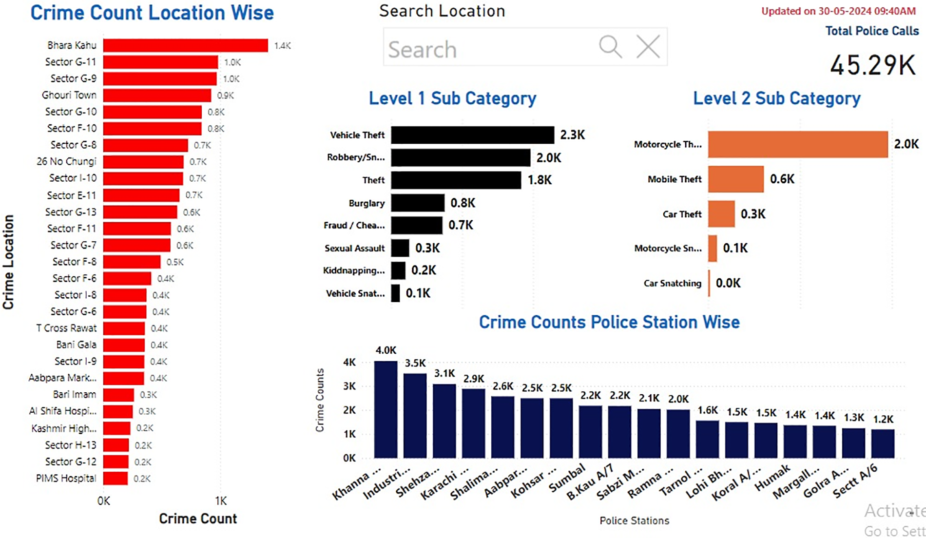
Figure 6: CHART based hotspot detection

Figure 7: Hotspot detection of week days

This allows for a more focused allocation of resources to the areas that need them the most, enhancing the overall safety of the community. Additionally, the dashboard provides insights into the most common types of crimes and their hotspots, which assists law enforcement agencies in prioritizing specific crime prevention strategies.

6  Conclusion and Future Work

This research proposes an advanced machine learning framework, CHART (Crime Hotspot Analysis and Real-time Tracking), designed to address the challenges in crime prediction and prevention. The methodology begins with comprehensive data collection from the ICT police database, encompassing detailed attributes such as crime type, location, time, and demographic information. Key steps include data preprocessing, domain-specific feature engineering, heat map generation using Kernel Density Estimation (KDE), and hotspot detection with a Random Forest model to predict crime likelihood in various areas. Experimental evaluation demonstrated CHART’s superior performance over benchmark methods, significantly improving crime detection accuracy, achieving 95.24% for CD-I, 96.12% for CD-II, and 94.68% for CD-III. The integration of sophisticated preprocessing techniques, balanced data representation, and advanced feature engineering ensures the model’s reliability and practicality for real-world crime analysis. Visualization of crime hotspots allows law enforcement agencies to strategize effectively, focusing resources on high-risk areas to enhance overall crime prevention and response efforts. Future work will explore incorporating real-time data streams, enhancing model adaptability to emerging crime patterns, and integrating additional contextual factors such as socio-economic indicators to further improve prediction accuracy and utility.

Acknowledgement: The authors extend their appreciation to King Saud University for funding this work.

Funding Statement: The authors extend their appreciation to King Saud University for funding this work through Researchers Supporting Project number (RSPD2025R685), King Saud University, Riyadh, Saudi Arabia.

Author Contributions: Rashid Ahmad: Paper Writing; Asif Nawaz: Methodology; Ghulam Mustafa: Formal Analysis; Tariq Ali: Experimental Analysis; Mehdi Tlija: Writing—Review & Editing; Mohammed A. El-Meligy: Supervision; Zohair Ahmed: Study Conception and Design. All authors reviewed the results and approved the final version of the manuscript.

Availability of Data and Materials: Not available.

Ethics Approval: Not applicable.

Conflicts of Interest: The authors declare no conflicts of interest to report regarding the present study.

References

1. C. S. Ogbodo, “Law, human rights, crime and society,” Afr. Hum. Rights Law J., vol. 8, no. 1, pp. 1–15, Jan. 2024. [Google Scholar]

2. F. A. Paul, A. A. Dangroo, and P. Saikia, “Societal and individual impacts of substance abuse,” J. Health Soc. Behav., vol. 10, no. 2, pp. 25–40, Feb. 2024. doi: 10.1007/978-3-030-68127-2. [Google Scholar] [CrossRef]

3. D. Birks, A. Coleman, and D. Jackson, “Unsupervised identification of crime problems from police free-text data,” Crime Sci., vol. 9, no. 1, pp. 1–18, 2020. doi: 10.1186/s40163-020-00127-4. [Google Scholar] [CrossRef]

4. M. J. Fortner and C. Stevens, Crime, Punishment, and Urban Criminal Justice Systems in the United States, Cheltenham, UK: Edward Elgar Publishing, 2024. [Google Scholar]

5. N. Shah, N. Bhagat, and M. Shah, “Crime forecasting: A machine learning and computer vision approach to crime prediction and prevention,” Vis. Comput. Ind., Biomed., Art, vol. 4, no. 1, pp. 9–18, 2021. [Google Scholar] [PubMed]

6. I. Fedchak, O. Kondratіuk, A. Movchan, and S. Poliak, “Theoretical foundations of hot spots policing and crime mapping features,” Soc. Legal Stud., vol. 1, no. 7, pp. 174–183, Jan. 2024. doi: 10.32518/sals1.2024.174. [Google Scholar] [CrossRef]

7. Y. Yan, W. Quan, and H. Wang, “A data-driven adaptive geospatial hotspot detection approach in smart cities,” Trans. GIS, vol. 28, no. 2, pp. 303–325, Feb. 2024. doi: 10.1111/tgis.13137. [Google Scholar] [CrossRef]

8. K. Mukherjee, S. Saha, S. Karmakar, and P. Dash, “Uncovering spatial patterns of crime: A case study of Kolkata,” Crime Prev. Community Saf., vol. 26, no. 1, pp. 47–90, Jan. 2024. doi: 10.1057/s41300-024-00198-4. [Google Scholar] [CrossRef]

9. I. Debata, P. S. Panda, E. Karthikeyan, and J. Tejas, “Spatial auto-correlation and endemicity pattern analysis of crimes against children in Tamil Nadu from 2017 to 2021,” J. Fam. Med. Prim. Care, vol. 13, no. 6, pp. 2341–2347, Jun. 2024. doi: 10.4103/jfmpc.jfmpc_1463_23. [Google Scholar] [PubMed] [CrossRef]

10. C. Massarelli and V. F. Uricchio, “The contribution of open source software in identifying environmental crimes caused by illicit waste management in urban areas,” Urban Sci., vol. 8, no. 1, Jan. 2024, Art. no. 21. doi: 10.3390/urbansci8010021. [Google Scholar] [CrossRef]

11. A. K. Selvan and N. Sivakumaran, “Crime detection and crime hot spot prediction using the BI-LSTM deep learning model,” Int. J. Knowl.-Based Dev., vol. 14, no. 1, pp. 57–86, Jan. 2024. doi: 10.1504/IJKBD.2024.137600. [Google Scholar] [CrossRef]

12. S. R. Bandekar and C. Vijayalakshmi, “Design and analysis of machine learning algorithms for the reduction of crime rates in India,” Procedia Comput. Sci., vol. 172, no. 1, pp. 122–127, 2020. doi: 10.1016/j.procs.2020.05.018. [Google Scholar] [CrossRef]

13. F. Dakalbab, M. A. Talib, O. A. Waraga, A. B. Nassif, S. Abbas and Q. Nasir, “Artificial intelligence crime prediction: A systematic literature review,” Social Sci. Human., vol. 6, no. 1, 2022, Art. no. 100342. [Google Scholar]

14. Y. Xie, S. Shekhar, and Y. Li, “Statistically-robust clustering techniques for mapping spatial hotspots: A survey,” ACM Comput. Surv., vol. 55, no. 2, pp. 1–38, Feb. 2022. [Google Scholar]

15. G. Garcia-Zanabria et al., “CriPAV: Street-level crime patterns analysis and visualization,” IEEE Trans. Vis. Comput. Graph., vol. 28, no. 12, pp. 4000–4015, Dec. 2021. doi: 10.1109/TVCG.2021.3111146. [Google Scholar] [PubMed] [CrossRef]

16. S. K. Al-Osaimi, “Survey of crime data analysis using the Apriori algorithm,” Know.-Based Syst., vol. 10, no. 1, pp. 454–498, 2021. [Google Scholar]

17. J. Wu, S. M. Abrar, N. Awasthi, E. Frias-Martinez, and V. Frias-Martinez, “Enhancing short-term crime prediction with human mobility flows and deep learning architectures,” EPJ Data Sci., vol. 11, no. 1, Feb. 2022, Art. no. 53. doi: 10.1140/epjds/s13688-022-00366-2. [Google Scholar] [PubMed] [CrossRef]

18. B. Cardone and F. Di Martino, “Fuzzy-based spatiotemporal hot spot intensity and propagation—an application in crime analysis,” Electronics, vol. 11, no. 3, Feb. 2022, Art. no. 370. doi: 10.3390/electronics11030370. [Google Scholar] [CrossRef]

19. S. K. Appiah, K. Wirekoh, E. N. Aidoo, S. D. Oduro, and Y. D. Arthur, “A model-based clustering of expectation-maximization and K-means algorithms in crime hotspot analysis,” Res. Math., vol. 9, no. 1, 2022, Art. no. 2073662. doi: 10.1080/27684830.2022.2073662. [Google Scholar] [CrossRef]

20. B. R. Prathap, “Geospatial crime analysis and forecasting with machine learning techniques,” Artif. Intell. Mach. Learn. EDGE Comput., vol. 1, no. 1, pp. 87–102, 2022. doi: 10.1016/B978-0-12-824054-0.00008-3. [Google Scholar] [CrossRef]

21. K. Malik, M. Pandey, A. Khan, and M. Srivastav, “Crime prediction by comparing machine learning and deep learning algorithms,” in 2024 2nd Int. Conf. Disrup. Technol. (ICDT), Noida, India, Mar. 2024, pp. 215–219. [Google Scholar]

22. O. Z. Apene, N. V. Blamah, and G. I. O. Aimufua, “Advancements in crime prevention and detection: From traditional approaches to artificial intelligence solutions,” Euro. J. Appl. Sci., Eng. Technol., vol. 2, no. 2, pp. 285–297, Feb. 2024. doi: 10.59324/ejaset.2024.2(2).20. [Google Scholar] [CrossRef]

23. A. Alsubayhin, M. S. Ramzan, and B. Alzahrani, “Crime prediction model using three classification techniques: Random forest, logistic regression, and LightGBM,” Int. J. Adv. Comput. Sci. Appl., vol. 15, no. 1, pp. 698–717, Jan. 2024. doi: 10.14569/issn.2156-5570. [Google Scholar] [CrossRef]

24. R. M. Aziz, P. Sharma, and A. Hussain, “Machine learning algorithms for crime prediction under Indian penal code,” Ann. Data Sci., vol. 11, no. 1, pp. 379–410, 2024. doi: 10.1007/s40745-022-00424-6. [Google Scholar] [CrossRef]

25. A. Sharma, R. Agarwal, and A. M. Nancy, “Detecting pattern in crime analysis using machine learning,” AIP Conf. Proc., vol. 3075, no. 1, pp. 1–8, Jul. 2024. [Google Scholar]

26. A. Alhudhaif, “A novel multi-class imbalanced EEG signals classification based on the adaptive synthetic sampling (ADASYN) approach,” PeerJ Comput. Sci., vol. 7, no. 1, 2021, Art. no. e523. doi: 10.7717/peerj-cs.523. [Google Scholar] [PubMed] [CrossRef]

27. T. Hart and P. Zandbergen, “Kernel density estimation and hotspot mapping,” Policing, vol. 37, no. 2, pp. 305–323, Jun. 2014. doi: 10.1108/PIJPSM-04-2013-0039. [Google Scholar] [CrossRef]

28. Y. Hu, F. Wang, C. Guin, and H. Zhu, “A spatio-temporal kernel density estimation framework for predictive crime hotspot mapping and evaluation,” Appl. Geogr., vol. 99, no. 1, pp. 89–97, May 2018. doi: 10.1016/j.apgeog.2018.08.001. [Google Scholar] [CrossRef]