
 Submit a Paper
 Propose a Special lssue
 Open Access
ARTICLE

Modeling and Predictive Analytics of Breast Cancer Using Ensemble Learning Techniques: An Explainable Artificial Intelligence Approach
1 Computer Science and Engineering Discipline, Khulna University, Khulna, 9208, Bangladesh
2 Information and Communication Engineering, Noakhali Science and Technology University, Noakhali, 3814, Bangladesh
3 School of Computing Sciences and Computer Engineering, University of Southern Mississippi, Hattiesburg, MS 39401, USA
4Computer Skills, Department of Self-Development Skill, Common First Year Deanship, King Saud University, Riyadh, 11362, Saudi Arabia
5 Computer Science Department, College of Computer and Information Sciences, King Saud University, Riyadh, 12372, Saudi Arabia
* Corresponding Author: Anupam Kumar Bairagi. Email:
(This article belongs to the Special Issue: Emerging Trends and Applications of Deep Learning for Biomedical Signal and Image Processing)
Computers, Materials & Continua 2024, 81(3), 4033-4048. https://doi.org/10.32604/cmc.2024.057415
Received 16 August 2024; Accepted 30 October 2024; Issue published 19 December 2024
 View Full Text
 Download PDF
Abstract
Breast cancer stands as one of the world’s most perilous and formidable diseases, having recently surpassed lung cancer as the most prevalent cancer type. This disease arises when cells in the breast undergo unregulated proliferation, resulting in the formation of a tumor that has the capacity to invade surrounding tissues. It is not confined to a specific gender; both men and women can be diagnosed with breast cancer, although it is more frequently observed in women. Early detection is pivotal in mitigating its mortality rate. The key to curbing its mortality lies in early detection. However, it is crucial to explain the black-box machine learning algorithms in this field to gain the trust of medical professionals and patients. In this study, we experimented with various machine learning models to predict breast cancer using the Wisconsin Breast Cancer Dataset (WBCD) dataset. We applied Random Forest, XGBoost, Support Vector Machine (SVM), Multi-Layer Perceptron (MLP), and Gradient Boost classifiers, with the Random Forest model outperforming the others. A comparison analysis between the two methods was done after performing hyperparameter tuning on each method. The analysis showed that the random forest performs better and yields the highest result with 99.46% accuracy. After performance evaluation, two Explainable Artificial Intelligence (XAI) methods, SHapley Additive exPlanations (SHAP) and Local Interpretable Model-Agnostic Explanations (LIME), have been utilized to explain the random forest machine learning model.Keywords
Abbreviations
| WBCD | Wisconsin Breast Cancer Dataset |
| KNN | K-Nearest Neighbour |
| XAI | Explainable artificial intelligence |
| SVM | Support Vector Machine |
| LIME | Local Interpretable Model-Agnostic Explanations |
| SHAP | Shapley Additive Explanations |
In recent times, breast cancer has surpassed lung cancer to emerge as the most widespread type of cancer globally [1]. Over 2 million new instances of breast cancer were documented worldwide in the year 2020 [2]. Although breast cancer can affect men, it is predominantly a disease that impacts women. It is the second leading cause of cancer-related deaths among women [3]. It is a form of cancer that originates in the cells of the breast, leading to uncontrolled cell growth. Lumps of the breast are classified as either malignant (cancerous) or benign (non-cancerous). Most women have benign breast conditions, which are very common. Benign tumors have unusual growths but do not spread beyond the breast. Although not life-threatening, some benign breast lumps can significantly raise a female’s risk of developing breast cancer. Malignant lumps, however, are dangerous and can result in various critical conditions, including death.
Benign and malignant conditions should be treated as soon as possible. For this reason, identifying breast cancer early on can be tremendously advantageous. However, the problem lies in the complexity of distinguishing between benign and malignant conditions in their early stages. Conventional diagnostic methods, such as mammograms, ultrasounds, and magnetic resonance imaging (MRI) scans, though widely used, often present challenges in accuracy due to overlapping features between benign and malignant tissues. This results in a high rate of false positives, leading to unnecessary biopsies, or false negatives, which delay the diagnosis of cancerous growths. Additionally, manual interpretation of these images is prone to human error and requires a high level of expertise. Detecting early-stage breast cancer is particularly challenging because it is often characterized by subtle and small changes that may be easily missed. To address these challenges, machine learning (ML) offers a promising solution. Machine learning algorithms have the ability to analyze large volumes of complex data, such as medical images and numerical data, and can learn to identify patterns that may not be immediately obvious to humans. By training on vast datasets, ML models can improve the accuracy of breast cancer detection, reducing both false positives and false negatives.
Diseases such as skin cancer [4], monkeypox [5], thyroid disorders [6], and COVID-19 [7] have been effectively detected using ML and deep learning (DL) techniques. The success of ML and DL in addressing these medical challenges stems from their ability to process vast amounts of structured data and analyze complex patterns in imaging and clinical data [8–10]. These models excel in feature extraction [11], automatically identifying subtle indicators that may not be apparent through traditional methods. Furthermore, ML and DL models are highly scalable, improving their performance as more data becomes available, which enhances the accuracy and efficiency of early disease detection. By leveraging these capabilities, ML and DL offer significant advancements in the timely and reliable diagnosis of various diseases.
Various ML techniques have been utilized in the diagnosis and prediction of breast cancer. In [12], the authors employed multiple machine-learning algorithms to classify breast cancer using three-dimensional images. Based on overall performance, they found that Support Vector Machine (SVM) was the best method. Authors of [13] combined the clustering method with an effective support vector machine algorithm and they used the Wisconsin Breast Cancer Corpus (WBCC). The authors of [14] conducted a comparative analysis of several machine learning approaches and determined that SVM is the most accurate classification algorithm. Also, Latchoumi et al. [15] introduced a weighted particle swarm optimization (WPSO) for classifying breast cancer. They utilized WPSO in conjunction with a smooth SVM. Even if a prediction system might be helpful, it is crucial to comprehend why the model has generated a particular prediction [16]. Explainable artificial intelligence (XAI) [17] techniques can be used to understand the model’s prediction by medical experts. XAI refers to techniques and approaches in the application of artificial intelligence methods that enable human experts to comprehend the results of the solution.
In this study, the post-hoc XAI methods have been considered. The post-hoc methods analyze the model after training without limiting the machine learning’s model complexity. Therefore, the model’s accuracy doesn’t get affected to achieve explainability. However, intrinsic methods restrict the complexity of the machine learning model. This study provides an explainable framework for classifying breast cancer on the WBCD dataset through learning. The subsequent points outline the significant contributions of this study:
• Firstly, a system model employing ensemble learning for classifying breast cancer on the WBCD dataset has been suggested.
• Secondly, global and local explainability have been provided using two XAI methods.
• Thirdly, the grid search technique was employed to optimize the models.
• Finally, the experimental results indicated that the suggested Random Forest model generates higher outcomes, achieving an accuracy of 99.46%.
The following sections of this study are methodically organized in the following way: Section 2 provides a comprehensive discussion of the existing literature. It explores various findings and perspectives within the field. Section 3 outlines different methodological steps, encompassing data collection, preprocessing techniques, architectural nuances of the model, integration of XAI methods, and the chosen evaluation approach. Section 4 focuses on result evaluation. It offers a comprehensive analysis of the outcomes derived from employing various ML techniques. Section 5 provides a conclusive summary.
2 Related Works on Breast Cancer Detection
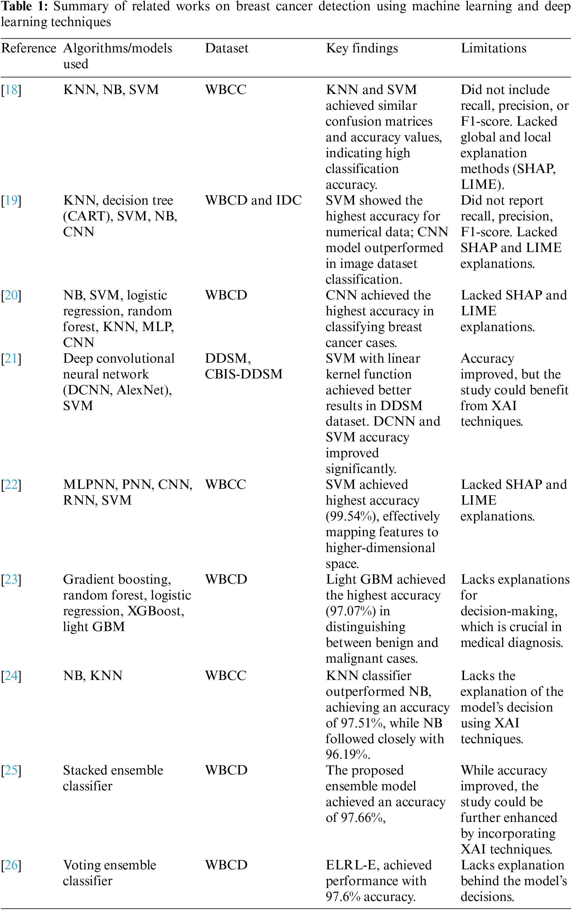
Breast cancer is a widespread and potentially life-threatening condition characterized by the abnormal proliferation of cells in the breast tissue. It stands as the most prevalent cancer among women globally and poses a significant public health concern. Detecting breast cancer early and making accurate predictions are essential for timely interventions and improved patient outcomes. Different methods in ML and DL have demonstrated potential in assisting with diagnosing breast cancer by examining crucial features extracted from medical imaging data. Table 1 presents a summary of works focused on breast cancer detection using machine learning and deep learning techniques.
The methodology section of this study details the procedural steps encompassing data collection, preprocessing, dataset partitioning, model architecture (Random Forest and XGBoost), and the evaluation metrics employed for assessing model performance. Additionally, the explanation techniques LIME and SHAP are discussed. Firstly, to achieve the objectives set out, the WBCD dataset is collected and pre-processed to ensure data uniformity. Afterwards, the model was trained using two ensemble learning. Then, with the validation set, hyperparameter tuning was done. For the hyperparameter tuning process, the grid search technique has been used. Then, the performance of the classifiers is evaluated using standard performance evaluation metrics such as precision, accuracy, recall, and F1-score. Finally, SHAP and LIME have been used to offer insights into the models’ interpretability. The schematic overview of the study’s workflow is depicted in Fig. 1.

Figure 1: Overall workflow diagram
3.1 Data Collection and Feature Explanation
For this study, the WBCD dataset published by the University of California, Irvine’s Center for Machine Learning and Intelligent Systems has been used [27]. The dataset consists of 569 patients’ data, and each instance has 32 features. Out of these, one is the target label (benign or malignant), and another is the patient’s identification number, leaving 30 features for input into the machine learning models. These features were derived from morphological patterns observed in cell nuclei, extracted from both benign and malignant tumors. Malignant tumors are typically characterized by larger, more irregular, and less symmetrical nuclei, with higher variability in both size and shape. Key features such as area, perimeter, concavity, compactness, and fractal dimension were specifically chosen to capture these pathological differences. For instance:
• Area, radius, and perimeter are generally larger in malignant cells due to uncontrolled growth.
• Smoothness and symmetry tend to be lower in malignant cells because their boundaries are irregular.
• Concavity and concave points are higher in malignant tumors due to the invasive nature of cancer cells, which tend to have irregular, inward-curved boundaries.
• Fractal dimension measures the complexity of the cell boundary, which is often higher in malignant tumors due to their abnormal growth patterns.
These features were carefully selected based on their relevance to the pathological differences between benign and malignant cells, providing a strong basis for classification models to differentiate between the two. The final column in the dataset denotes whether the patient is afflicted with benign or malignant tumors. Out of the 569 instances, 357 are classified as benign and 212 as malignant.
Data preprocessing plays a pivotal role in optimizing machine learning model performance. It refines input data to enhance accuracy and compatibility with model training.
It’s common for real-world datasets to have missing values. These gaps in the data can negatively impact model training. Various methods can be employed to address this issue, such as imputing missing values with the mean, median, or mode of the respective feature. This ensures that the dataset is complete and ready for analysis. As a crucial step in data quality assurance, an assessment was conducted to verify the presence of missing values within the dataset. It is pertinent to highlight that this evaluation affirmatively establishes the absence of any missing values across all instances.
3.2.2 Encoding Categorical Variables
Machine learning models require numerical input, so categorical variables (like “benign” and “malignant”) need to be transformed. One-hot encoding is a method that translates categorical variables into binary columns, assigning a value of either 1 or 0 to indicate each category. This allows the model to process categorical data effectively.
The dataset has been split using the holdout method. 33% of the data has been kept in the testing set, while the remaining data has been preserved in the training set. Next, we conducted 3-fold cross-validation on the training set and utilized the best-performing model for further evaluation. In this study, we chose Random Forest, Gradient Boost, XGBoost, SVM, and MLP for classification due to their proven effectiveness in various applications.
For the classification process, we employed three ensemble learning techniques: Random Forest, XGBoost, and Gradient Boost, along with SVM and MLP.
Random Forest [28] is an ensemble ML approach that constructs numerous decision trees and amalgamates their outputs to generate predictions. The predictions of the individual trees are combined through a process known as majority voting (for classification) or averaging (for regression). In our study, the parameters for the Random Forest model were fine-tuned using a grid search to optimize performance. The selected parameters were: bootstrap set to True, max_depth set to None, min_samples_leaf set to 1, min_samples_split set to 2, and n_estimators set to 200. The total execution time for the Random Forest model was 21.21 s. These parameters were chosen to construct trees of sufficient depth to capture complex patterns while maintaining a relatively high number of estimators (trees) to improve prediction accuracy and robustness. Allowing a minimum sample size of 2 for node splits contributed to deeper trees, further enhancing the model’s ability to capture intricate details in the dataset.
Gradient Boost [29] is a machine learning approach used for regression and classification challenges, generating a predictive model as an ensemble of weak prediction models, usually in the form of decision trees. In our study, the tuned parameters were: learning_rate set to 0.2, max_depth set to 3, subsample set to 0.6, and n_estimators set to 300. The total execution time for the Gradient Boost model was 57.50 s.
XGBoost [30] is an advanced machine-learning algorithm that extends the principles of gradient boosting for regression and classification problems. Like gradient boosting, XGBoost constructs a predictive model as an ensemble of weak prediction models, typically decision trees. For the XGBoost model, the parameters used were: colsample_bytree set to 0.8, learning_rate set to 0.4, max depth set to None, subsample set to 0.5, and n_estimators set to 100. The XGBoost model’s execution time was 13.96 s.
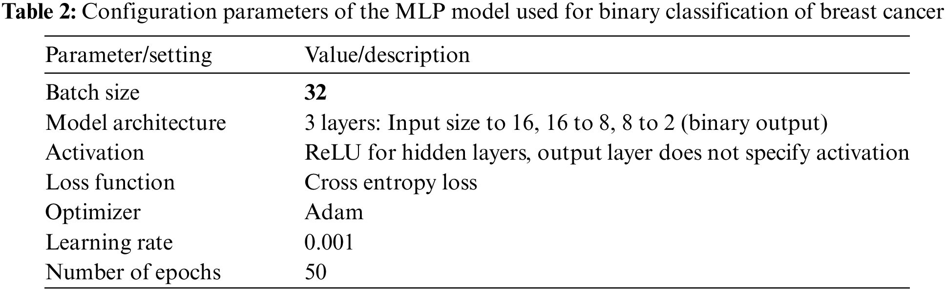
Multi-Layer Perceptron (MLP) is a class of feedforward artificial neural networks that is highly effective for various classification and regression tasks. For this study, the parameters of the used MLP models are given as follows in Table 2. The MLP’s execution time was 0.77 s.
Support Vector Machines (SVM) is a robust classification technique effective for both binary and multi-class problems. SVM works by finding a hyperplane that best separates the data points into different classes with the maximum possible margin, which enhances the model’s generalization capabilities. We used the rbf-kernel for the SVM model. The C value and gamma were set to 10 and 0.01, respectively. SVM’s execution time was 0.23 s. The random state for all experiments was set to 551,398 using a randomization function.
For the explainability Local Interpretable Model-Agnostic Explanations (LIME) [31] and Shapley Additive Explanations (SHAP) have been used [32].
This study employs a comprehensive set of five evaluation metrics to gauge performance and method effectiveness. The metrics under consideration include Precision, Recall, F1-score, and Accuracy, each contributing a distinct perspective to the assessment.
In the result analysis, we thoroughly evaluate the performance of the models using several machine learning techniques: Random Forest and Gradient Boost, XGBoost, MLP and SVM. The models’ effectiveness is assessed based on various evaluation metrics, including confusion matrices, accuracy, precision, recall, and F1-score. Additionally, two XAI techniques, SHAP and LIME, are employed to provide deeper insights into the models’ decision-making processes. This combination of performance evaluation and interpretability not only enhances our understanding of the models’ behavior but also highlights the study’s focus on delivering transparent, interpretable, and clinically meaningful insights.
4.1 Comparison of Model Evaluation Metrics for Breast Cancer Classification
The comparative performance of our classification models is detailed in Table 3, highlighting the key metrics: accuracy, precision, recall, and F1-scores. This comprehensive analysis provides insights into each model’s effectiveness in distinguishing between benign and malignant breast cancer cases.
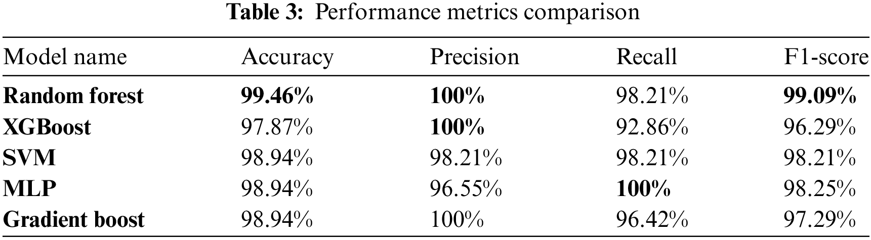
Table 4 presents in this study provides a comprehensive comparison of various parameter values, performance metrics (precision, recall, F1-score, and accuracy), as well as local and global explanations for breast cancer prediction. By juxtaposing our findings with those from existing studies, we have gained valuable insights into the effectiveness of different parameter configurations and the interpretability of the models. This analysis reinforces the significance of our research and contributes to the existing knowledge in the field of breast cancer prediction using ML techniques. This analysis shows that our proposed method stands out with the highest accuracy, underlining its ability to correctly classify breast cancer cases.
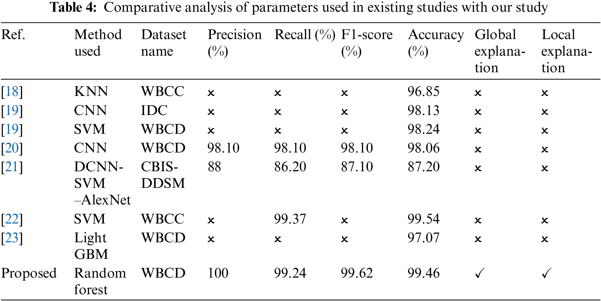
Furthermore, the model demonstrates strong precision, indicating a low number of false positives. Its high recall reflects the ability to detect a significant proportion of malignant cases, contributing to its effectiveness. The F1-score, which balances precision and recall, highlights the model’s overall performance. Additionally, the method enhances interpretability by employing LIME for localized model understanding and SHAP for explaining global feature importance. This combination of accuracy and interpretability makes the approach well-suited for breast cancer classification, offering a comprehensive and reliable method for improving diagnosis and treatment.
In this study, we focus on the Random Forest model due to its superior performance, featuring both global and local explainability. Global explainability offers a comprehensive overview of the model’s behavior, identifying key features that significantly influence predictions across all cases, which helps in understanding the general impact of each feature on model decisions.
In our study, SHAP was employed to provide a global explanation of the model’s decision-making process, as depicted in Fig. 2. This analysis identified the worst perimeter as the most influential feature across both malignant and benign cases, underscoring its pivotal role in the classification process. The worst perimeter measures the boundary length of the tumor; larger perimeters often indicate more irregular and potentially aggressive growth patterns associated with malignancy. Following closely in importance were worst area, worst concave points, worst radius, and mean concave points.

Figure 2: Features impact on random forest model’s output
The worst area quantifies the largest tumor area, with larger areas typically correlating with malignancy due to extensive tumor growth. The worst concave points reflect the number of indentations or irregularities on the tumor surface, where higher values suggest a more invasive and malignant nature. The worst radius measures the maximum distance from the tumor center to its perimeter, with larger radii often indicating aggressive growth. Mean concave points average the concave points across the tumor, providing a comprehensive view of its irregularity.
Fig. 3a illustrates the impact of these features on the classification of instances as malignant. It is evident that higher values in worst perimeter, worst area, worst concave points, worst radius, and mean concave points increase the probability of a tumor being classified as malignant. This aligns with clinical understandings that larger, more irregular tumors are more likely to be cancerous. Conversely, Fig. 3b demonstrates that these same features have a negative impact on benign classifications. Specifically, lower values in these parameters reduce the likelihood of a tumor being benign, reinforcing the model’s reliance on these critical markers for accurate diagnosis.

Figure 3: Features impact. (a) Malignant class. (b) Benign class
Overall, the SHAP analysis underscores the model’s dependence on key geometric and textural features of tumors. Features indicating larger size and greater irregularity consistently influence the model toward malignancy, while smaller, smoother tumors are more likely to be classified as benign. These insights not only validate the model’s alignment with clinical diagnostic criteria but also highlight the importance of these features in developing reliable breast cancer prediction systems. The global explanation provided by SHAP facilitates a deeper understanding of feature dynamics, guiding future clinical assessments and model enhancements to improve diagnostic accuracy.
LIME has been utilized to provide local explanations for the model’s predictions on breast cancer classification. As depicted in Fig. 4, the impact of specific features on several instances can be visualized, offering insights into how the model arrived at its decisions. In Fig. 4a, the model predicted the instance as malignant with a 59% probability. The most influential feature was worst concavity, which measures the largest degree of inward curvature of the tumor boundary. A higher concavity indicates a more irregular and invasive tumor shape, commonly associated with malignancy. In this instance, the worst concavity value was 0.83, exceeding the threshold of 0.49, strongly impacting the prediction of malignancy. Similarly, the worst concave points, representing the number of concave portions in the tumor contour, had a high value of 0.72, suggesting numerous sharp indentations—another characteristic linked to malignant tumors.

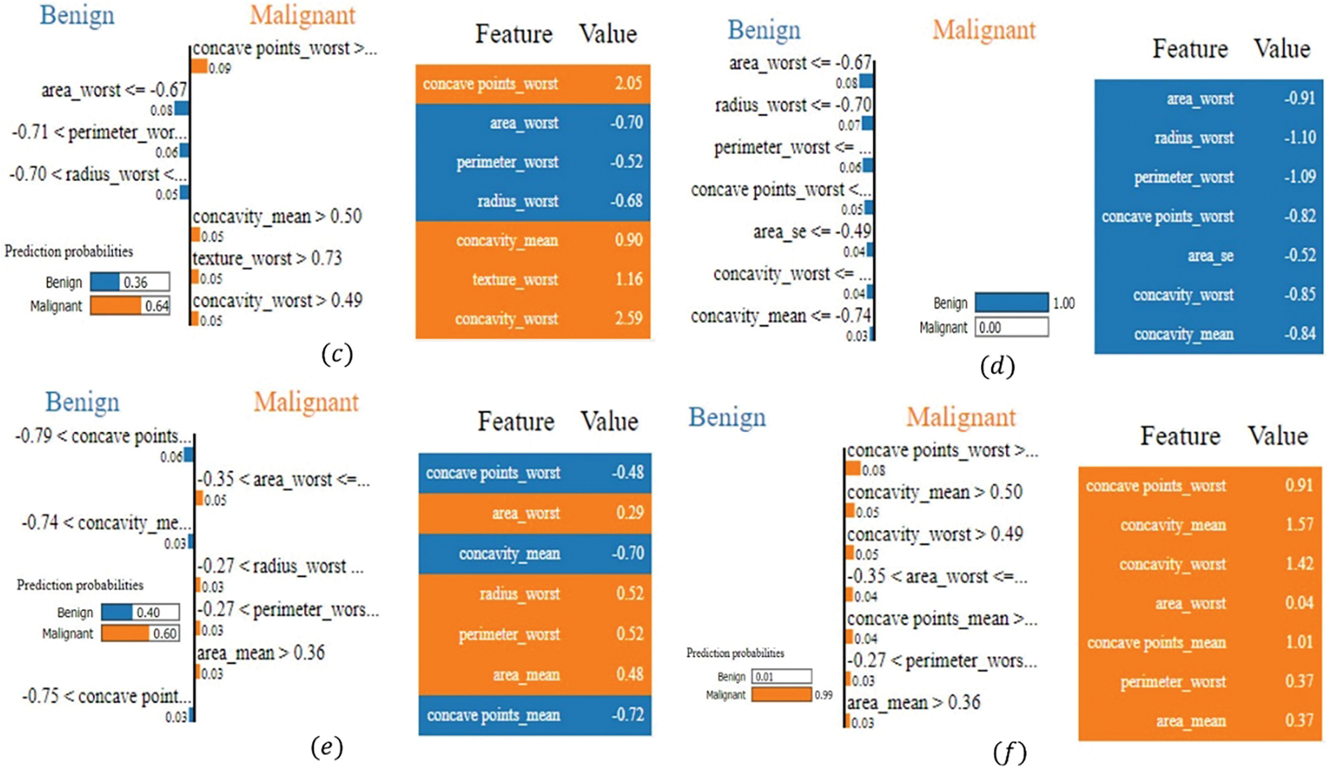
Figure 4: LIME-based explanations for the model’s breast cancer classification predictions, showing key feature contributions across various instances: (a) the instance predicted as malignant (59% probability), influenced by high values of the worst concavity and the worst concave points; (b) the instance predicted as benign (99% probability), influenced by low values of the worst area, worst radius, and worst perimeter; (c) the instance predicted as malignant (64% probability), with conflicting benign and malignant features; concavity values indicate malignancy; (d) the instance predicted as benign (97% probability), influenced by consistently low values in size and shape metrics; (e) the instance predicted as malignant (99% probability), influenced by high values of worst concave points and concavity features. (f) the instance predicted as malignant (99% probability), with concave points and concavity values indicating malignancy
In Fig. 4b, the model confidently classified the instance as benign with a 99% probability. The key contributing feature was the worst area (−0.70), which represents the largest area of the tumor observed. Lower values suggest a smaller tumor size, less indicative of malignancy due to the limited growth associated with benign tumors. This value was below the threshold of −0.67, significantly influencing the benign prediction. Similarly, the worst radius (−0.77), measuring the largest distance from the tumor center to its perimeter, and the worst perimeter (−0.76), indicating the largest boundary length, also had low values. These features suggest a smaller, less aggressive tumor, reinforcing the benign classification. The combination of low values in these size-related features led the model to confidently classify the instance as benign, indicating the tumor lacks characteristics typical of malignancy. In Fig. 4c, the model predicted malignant with a 64% probability, while 36% suggested benignity, highlighting a contrast between features contributing to both outcomes. For the malignant prediction, worst concave points had the highest influence, with a value of 2.05, indicating numerous sharp indentations on the tumor surface—a hallmark of malignant, irregular growth. Worst concavity (2.59) and mean concavity (0.90) also had high values, suggesting pronounced inward curvature and overall irregularity in the tumor shape, contributing to the malignancy prediction. Conversely, features such as worst area (−0.70), worst radius (−0.68), worst perimeter (−0.52), and area SE (−0.58) had lower values, contributing towards a benign classification. These features indicate a smaller tumor size and simpler boundary, characteristics typical of benign tumors. The model weighed these conflicting indicators, and the significant irregularity suggested by the high concavity measures ultimately tipped the balance towards a malignant prediction.
In Fig. 4d, the model predicted the instance as benign with a high 97% probability. Influential features included worst area (−1.10), worst radius (−1.43), and worst perimeter (−1.38), all significantly low values indicating a small tumor size and simple boundary—features associated with benign tumors. These features strongly contributed to the benign classification. Additionally, the worst concave points (−1.39) and worst concavity (−0.92) had low values, suggesting minimal indentations and inward curvature, reinforcing the benign prediction. The model’s decision was driven by consistently low values in size and shape irregularity metrics, pointing towards a non-invasive, benign tumor. In Fig. 4e, the model’s prediction was malignant with a 99% probability, with only 1% indicating benignity. Key features influencing this decision were worst concave points (0.91), mean concavity (1.57), worst concavity (1.42), and mean concave points (1.01), all with high values indicating pronounced irregularity and invasiveness of the tumor boundary. These features are strong indicators of malignancy, reflecting abnormal cell growth and aggressive tumor behavior. Additional features like worst area (0.04), worst perimeter (0.37), and mean area (0.37) modestly supported malignancy by suggesting a larger tumor size. The combination of high values in both size and shape irregularity features led to the model’s strong confidence in predicting a malignant classification. In Fig. 4f, LIME elucidates the model’s prediction of malignant with a high 99% probability, contrasting sharply with the mere 1% probability for benign. The most influential feature driving this malignancy prediction was the worst concave points, which had a value of 0.91 and contributed 0.09 towards malignancy. As previously mentioned, this feature quantifies the number of indentations or concave regions on the tumor surface; higher values indicate a more irregular and invasive tumor boundary, typical of malignant growths. Additionally, mean concavity and worst concavity, with values of 1.57 and 1.42, respectively, contributed 0.05 and 0.04 to the malignant classification. Furthermore, mean concave points, valued at 1.01, added 0.04 towards malignancy, reflecting similar irregular surface patterns synonymous with cancerous tumors. Features such as worst area, worst perimeter, and the mean area also played supportive roles, contributing 0.04, 0.04, and 0.03, respectively. Although their values (0.37, 0.37, and 0.04) are relatively moderate, they indicate larger tumor sizes, which are often associated with malignancy due to more extensive and potentially aggressive growth.
The analysis demonstrates that the model relies heavily on features capturing the geometric and morphological properties of tumors. High values in features like concavity and concave points consistently indicated malignancy due to their association with irregular and invasive tumor boundaries. These features reflect the physical irregularities in tumor shape that are characteristic of malignant growths. Conversely, lower values in these features supported benign classifications, reflecting smoother and less invasive tumor shapes typical of non-cancerous growths. Similarly, features related to tumor size—such as worst area, worst radius, and worst perimeter—significantly influenced predictions. Larger sizes leaned toward malignancy, aligning with the understanding that malignant tumors often grow more rapidly and extensively. Smaller sizes supported benign outcomes, consistent with the nature of benign tumors, which tend to grow slowly and remain localized. An interesting finding is the model’s ability to balance conflicting features, as seen in Fig. 4c, where indicators of both malignancy and benignity were present.
In this study, we experimented with various machine learning models to predict breast cancer using the WBCD. We applied Random Forest, XGBoost, SVM, MLP, and Gradient Boosting classifiers, with the Random Forest model outperforming the others by achieving an impressive accuracy of 99.46%. Due to its strong performance, we employed SHAP for global interpretability and LIME for local explanations, ensuring that the model’s decisions are transparent and understandable. Continued research and refinement could lead to more reliable and interpretable systems for clinical use, ultimately contributing to better diagnostic outcomes and patient care.
Acknowledgement: The authors would like to thank King Saud University, Riyadh, Saudi Arabia for supporting the work by the Researchers Supporting Project (RSPD2024R846).
Funding Statement: This research was supported by the Researchers Supporting Project (RSPD2024R846), King Saud University, Riyadh, Saudi Arabia.
Author Contributions: The manuscript was written with contributions from all authors. Avi Deb Raha: Conceptualization, Methodology, and Writing—Original Draft Preparation. Fatema Jannat Dihan: Conceptualization, Methodology, and Writing—Original Draft Preparation. Mrityunjoy Gain: Conceptualization, Methodology, and Writing—Original Draft Preparation. Saydul Akbar Murad: Software, Data Curation, and Writing–Original Draft Preparation. Apurba Adhikary: Data Curation, and Investigation. Md. Bipul Hossain: Investigation, and Supervision. Md. Mehedi Hassan: Investigation, and Writing—Reviewing and Editing. Taher Al-Shehari, Nasser A Alsadhan, Mohammed Kadrie: Writing—Reviewing and Editing, and Funding. Anupam Kumar Bairagi: Supervision, and Writing—Reviewing and Editing. All authors reviewed the results and approved the final version of the manuscript.
Availability of Data and Materials: The Breast Cancer Wisconsin (Diagnostic) dataset published by the University of California, Irvine’s Center for Machine Learning and Intelligent Systems has been used for this study and it is publicly available. URL: https://archive.ics.uci.edu/ml/datasets/Breast+Cancer+Wisconsin+%28Diagnostic%29, accessed on 25 October 2024.
Ethics Approval: Not applicable.
Conflicts of Interest: The authors declare no conflicts of interest to report regarding the present study.
References
1. E. Arzanova and H. N. Mayrovitz, The Epidemiology of Breast Cancer. Brisbane, Australia: Exon Publications, 2022, pp. 1–19. [Google Scholar]
2. J. Ferlay et al., “Cancer statistics for the year 2020: An overview,” Int. J. Cancer, vol. 149, no. 4, pp. 778–789, 2021. doi: 10.1002/ijc.33588. [Google Scholar] [PubMed] [CrossRef]
3. C. E. DeSantis et al., “Breast cancer statistics, 2019” CA Cancer J. Clin., vol. 69, no. 6, pp. 438–451, 2019. doi: 10.3322/caac.21583. [Google Scholar] [PubMed] [CrossRef]
4. M. Suleman et al., “Smart MobiNet: A deep learning approach for accurate skin cancer diagnosis,” Comput. Mater. Contin., vol. 77, no. 3, pp. 3533–3549, 2023. doi: 10.32604/cmc.2023.042365. [Google Scholar] [CrossRef]
5. A. D. Raha et al., “Attention to monkeypox: An interpretable monkeypox detection technique using attention mechanism,” IEEE Access, vol. 12, pp. 51942–51965, 2024. doi: 10.1109/ACCESS.2024.3385099. [Google Scholar] [CrossRef]
6. M. B. Hossain et al., “An explainable artificial intelligence framework for the predictive analysis of hypo and hyper thyroidism using machine learning algorithms,” Human-Centric Intell. Syst., vol. 3, no. 3, pp. 211–231, 2023. [Google Scholar]
7. S. Akbar, H. Azam, S. S. Almutairi, O. Alqahtani, H. Shah and A. Aleryani, “Contemporary study for detection of COVID-19 using machine learning with explainable AI,” Comput. Mater. Contin., vol. 80, no. 1, pp. 1075–1104, 2024. doi: 10.32604/cmc.2024.050913. [Google Scholar] [CrossRef]
8. M. A. Islam, M. Z. H. Majumder, M. A. Hussein, K. M. Hossain, and M. S. Miah, “A review of machine learning and deep learning algorithms for Parkinson’s disease detection using handwriting and voice datasets,” Heliyon, vol. 10, no. 3, 2024, Art. no. e25469. doi: 10.1016/j.heliyon.2024.e25469. [Google Scholar] [PubMed] [CrossRef]
9. Z. Yao, F. Lin, S. Chai, W. He, L. Dai and X. Fei, “Integrating medical imaging and clinical reports using multimodal deep learning for advanced disease analysis,” 2024, arXiv:2405.17459. [Google Scholar]
10. M. G. Alsubaie, S. Luo, and K. Shaukat, “Alzheimer’s disease detection using deep learning on neuroimaging: A systematic review,” Mach. Learn. Knowl. Extr., vol. 6, no. 1, pp. 464–505, 2024. doi: 10.3390/make6010024. [Google Scholar] [CrossRef]
11. M. Gain, A. D. Raha, and R. Debnath, “CCC++: Optimized color classified colorization with segment anything model (SAM) empowered object selective color harmonization,” 2024, arXiv:2403.11494. [Google Scholar]
12. S. Nayak and D. Gope, “Comparison of supervised learning algorithms for RF-based breast cancer detection,” in 2017 Comput. Electromagnetics Int. Workshop (CEM), Barcelona, Spain, 2017, pp. 13–14. doi: 10.1109/CEM.2017.7991863. [Google Scholar] [CrossRef]
13. A. H. Osman, “An enhanced breast cancer diagnosis scheme based on two-step-SVM technique,” Int. J. Adv. Comput. Sci. Appl., vol. 8, no. 4, pp. 158–165, 2017. [Google Scholar]
14. Y. Khourdifi and M. Bahaj, “Applying best machine learning algorithms for breast cancer prediction and classification,” Proc. 2018 Int. Conf. Electron., Control, Optim. Comput. Sci. (ICECOCS), vol. 9, pp. 1–5, 2018. doi: 10.1109/ICECOCS.2018.8610632. [Google Scholar] [CrossRef]
15. T. P. Latchoumi and L. Parthiban, “Abnormality detection using weighed particle swarm optimization and smooth support vector machine,” Biomed. Res., vol. 28, no. 11, pp. 4749–4751, 2017. [Google Scholar]
16. S. Madapatha and P. Fernando, “A systematic literature review of XAI-based approaches on brain disease detection using brain MRI images,” in Proc. 2024 4th Int. Conf. Adv. Res. Comput. (ICARC), 2024, pp. 19–24. doi: 10.1109/ICARC61713.2024.10499752. [Google Scholar] [CrossRef]
17. A. N. Zereen, A. Das, and J. Uddin, “Machine fault diagnosis using audio sensors data and explainable AI techniques-LIME and SHAP,” Comput. Mater. Contin., vol. 80, no. 3, pp. 3463–3484, 2024. doi: 10.32604/cmc.2024.054886. [Google Scholar] [CrossRef]
18. B. Akbugday, “Classification of breast cancer data using machine learning algorithms,” in 2019 Medical Technol. Congr. (TIPTEKNO), Izmir, Turkey, 2019, pp. 1–4. doi: 10.1109/TIPTEKNO.2019.8895222. [Google Scholar] [CrossRef]
19. V. Apoorva, H. K. Yogish, and M. L. Chayadevi, “Breast cancer prediction using machine learning techniques,” in Proc. 3rd Int. Conf. Integr. Intell. Comput. Commun. Secur. (ICIIC), pp. 348–355, 2021. doi: 10.2991/ahis.k.210913.043. [Google Scholar] [CrossRef]
20. C. Shahnaz, J. Hossain, S. A. Fattah, S. Ghosh, and A. I. Khan, “Efficient approaches for accuracy improvement of breast cancer classification using wisconsin database,” in 2017 IEEE Region 10 Humanitarian Technol. Conf. (R10-HTC), Dhaka, Bangladesh, 2017, pp. 792–797. doi: 10.1109/R10-HTC.2017.8289075. [Google Scholar] [CrossRef]
21. D. A. Ragab, M. Sharkas, S. Marshall, and J. Ren, “Breast cancer detection using deep convolutional neural networks and support vector machines,” PeerJ, vol. 7, no. 5, 2019, Art. no. e6201. doi: 10.7717/peerj.6201. [Google Scholar] [PubMed] [CrossRef]
22. E. D. Übeyli, “Implementing automated diagnostic systems for breast cancer detection,” Expert Syst. Appl., vol. 33, no. 4, pp. 1054–1062, 2007. [Google Scholar]
23. R. Kiran, T. M. Rajesh, M. G. Krishna, N. Gopal, and G. Kishan, “Breast cancer classification using machine learning,” Int. Res. J. Adv. Sci. Hub., vol. 5, no. 5, pp. 88–93, 2023. doi: 10.47392/irjash.2023.S012. [Google Scholar] [CrossRef]
24. M. Amrane, S. Oukid, I. Gagaoua, and T. Ensarİ, “Breast cancer classification using machine learning,” in 2018 Electric Electronics, Computer Science, Biomedical Engineerings’ Meeting (EBBT), Istanbul, Turkey: Computer Science, pp. 1–4, 2018. [Google Scholar]
25. A. Sharma, D. Goyal, and R. Mohana, “An ensemble learning-based framework for breast cancer prediction,” Decis. Anal. J., vol. 10, no. 2, 2024, Art. no. 100372. doi: 10.1016/j.dajour.2023.100372. [Google Scholar] [CrossRef]
26. A. Batool and Y. -C. Byun, “Toward improving breast cancer classification using an adaptive voting ensemble learning algorithm,” IEEE Access, vol. 12, pp. 12869–12882, 2024. doi: 10.1109/ACCESS.2024.3356602. [Google Scholar] [CrossRef]
27. D. Dua and C. Graff, UCI Machine Learning Repository. Irvine, CA, USA: University of California, 2017. Accessed: Jun. 30, 2024. [Online]. Available: https://archive.ics.uci.edu [Google Scholar]
28. L. Breiman, “Random forests,” Mach. Learn., vol. 45, no. 1, pp. 5–32, 2001. doi: 10.1023/A:1010933404324. [Google Scholar] [CrossRef]
29. J. H. Friedman, “Stochastic gradient boosting,” Comput. Stat. Data Anal., vol. 38, no. 4, pp. 367–378, 2002. doi: 10.1016/S0167-9473(01)00065-2. [Google Scholar] [CrossRef]
30. T. Chen and C. Guestrin, “XGBoost: A scalable tree boosting system,” in Proc. 22nd ACM SIGKDD Int. Conf. Knowl. Discov. Data Min., KDD ’16, New York, NY, USA, Association for Computing Machinery, 2016, pp. 785–794. [Google Scholar]
31. M. T. Ribeiro, S. Singh, and C. Guestrin, “‘Why should I trust you?’ Explaining the predictions of any classifier,” in Proc. 22nd ACM SIGKDD Int. Conf. Knowl. Discov. Data Min., KDD ’16, New York, NY, USA, Association for Computing Machinery, 2016, pp. 1135–1144. [Google Scholar]
32. S. Lundberg, “A unified approach to interpreting model predictions,” 2017, arXiv:1705.07874. [Google Scholar]
Cite This Article
 Copyright © 2024 The Author(s). Published by Tech Science Press.
This work is licensed under a Creative Commons Attribution 4.0 International License , which permits unrestricted use, distribution, and reproduction in any medium, provided the original work is properly cited.
 Downloads
 Citation Tools