A Fine-Grained Defect Prediction Method Based on Drift-Immune Graph Neural Networks

1  Introduction

Software defect prediction (SDP) is a method that supports the use of metric metadata from software modules to detect defective modules in advance during the software development process. SDP can help developers and testers rationally allocate limited resources and provide techniques for software quality assurance [1].

In recent years, researchers have proposed many static analysis methods [2] for defect prediction that have achieved good results. Static analysis tools check for the presence of defects in software applications using predefined rules for detecting possible defects without executing the code. However, the formulation of well-defined rules relies strongly on expert knowledge. Not only is the formulation of these rules labour-intensive, it also difficult for these rules to address all defect cases. Static analysis tool efficiency is greatly reduced by the complex programming logic of the software in realistic development scenarios [3]. With the recent rapid development of artificial intelligence techniques, researchers have gradually begun using machine learning (ML) [4,5] and deep learning (DL) [6] techniques for SDP to mine hidden defect features in software. Compared to static analysis tools, ML- and DL-based methods require little or no expert knowledge to increase the efficiency of SDP. However, existing SDP methods still face two major limitations of these existing SDP methods.

Data drift (DD) in SDP has not been efficiently solved. In previous within-project defect prediction (WPDP) studies, models were typically trained by building a model on the first version of a project and then using it to predict all subsequent versions of the project. However, an empirical study by Wang et al. [7] showed that the performance of SDP models usually varies over time. Significant differences may exist in the data distributions of different versions of datasets. Generally, prediction models constructed on the datasets released in earlier versions are likely to suffer from degraded performance on datasets released in later versions owing to data drift during software evolution [8]. Wang et al. [7] proposed to use the evolution of data distribution characteristics to guide the reuse or updating of models. Although this approach achieves better prediction performance on subsequent software versions, it requires a tedious and time-consuming process of determining the distribution differences for each version to be predicted after the model construction. The required effort for addressing version differences would be greatly reduced by solving the data drift problem at the model level.

Most deep learning-based SDP methods exhibit coarse granularity of prediction. Researchers have studied defect prediction models at different granularities (e.g., packages [9], files [10,11], methods [12], and commits [13]). Currently, most existing SDP methods are granular at the file level, which is considered a coarse-grained approach. This means that when these methods are used to predict software defects, they can only determine whether a file is likely to contain defects and cannot determine which specific code statements are critical factors that may lead to defects. Statistically, typically only 1%–3% of code statements in a file are defective [14], indicating that when a file is predicted to be defective, developers may waste considerable time and effort in further identifying the high-risk lines of code in the file. Therefore, in the SDP approach, fine-grained results can help developers locate and fix defects more quickly and precisely, thus improving software quality.

To address the above issues, we propose an SDP method that effectively mitigates data drift at the model level. Unlike the previous deep learning-based SDP methods, our method focuses on effective mitigating of data drift and achievement of statement-level defect prediction. Even in the case of significant changes in subsequent software versions, our method can maintain good model performance. Moreover, the fine-grained prediction results can help developers locate and fix defects more efficiently.

An example of motivation. We present a simple example to illustrate how this paper applies graph learning to achieve robustness against software data distribution differences and to enable fine-grained defect prediction. As shown in Fig. 1, the code demonstrates the process of adding and removing elements from an ArrayList. The original implementation attempts to remove the last element of the list before adding any elements, which leads to an IndexOutOfBoundsException because the list is initially empty. The corrected version addresses this issue by first adding an element to the list before performing the removal operation. This ensures that the list contains at least one element, thereby preventing the exception and allowing the method to execute safely.

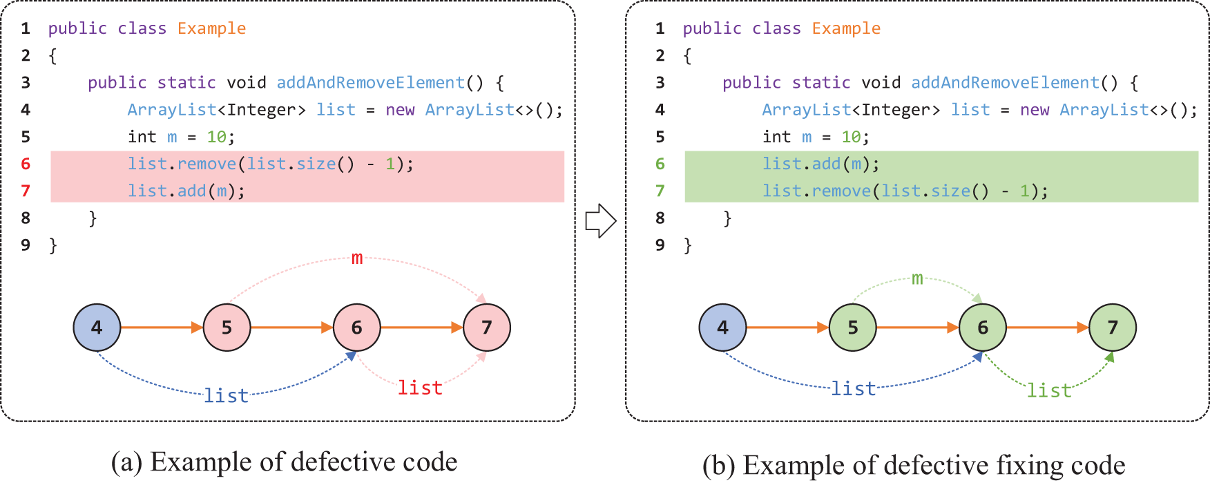
Figure 1: A motivating Java code example

The diagrams in Fig. 1 correspond to the program dependence graphs (PDGs) of the two code snippets. The dashed lines represent data flow, whereas the solid lines represent control flow. In Fig. 1a, the data flow from Statement 5 to Statement 7, and from Statement 6 to Statement 7, contributes to the defect (note that the control dependence between Statements 6 and 7 is not the key factor). The correct execution should follow the data flow from Statement 5 to Statement 6, and then from Statement 6 to Statement 7, as shown in Fig. 1b. Previous graph neural network (GNN) models often rely on the entire program dependence graph for defect prediction, which inadvertently includes irrelevant statements and dependencies, leading to biased predictions. By contrast, the method proposed in this paper identifies defect-related statements (represented as subgraph structures in the PDG, such as the data dependencies from 5->7 and 6->7 in Fig. 1a). By excluding the features unrelated to the defect labels, this approach improves robustness against data distribution shifts, enhancing the prediction accuracy. Moreover, this subgraph can be viewed as a set of statements that are highly relevant to the defect labels, indicating a higher likelihood of contributing to defect predictions. By focusing on these critical subgraph structures, the model improves its ability to accurately predict defects because captures the most important dependencies related to the target defect.

Solving the data drift problem in SDP based on information bottleneck (IB) theory and graph stochastic attention mechanism. To alleviate the data distribution differences between training and test data that arise during software evolution, we capture the most critical subgraph information related to defects in the graph representation based on the information bottleneck theory. This ensures that the model still shows stable prediction performance when its data distribution changes. In the graph learning process, we introduce the graph stochastic attention mechanism [15] for building graph neural networks (GNN) with excellent generalization ability. The basic principle of graph stochastic attention is derived from the concept of the information bottleneck [16,17]. It is formulated as an information bottleneck by introducing attention randomness to control the flow of information from the input graph to the prediction. During the training process, the randomness of the defect-independent graph components is kept constant, whereas the randomness of the defect-related graph components is automatically reduced. Graph stochastic attention can improve generalization by penalizing the amount of information in the input data; this difference also provides excellent interpretable power for the model. In this paper, we refer to the constructed GNN as a drift-immune graph neural network (DI-GNN). It effectively mitigates the data drift problem at the model level by capturing a distribution-independent defect-related subgraph. Specifically, we first construct a program dependency graph (PDG) for the source code files and further embed the code statements (i.e., nodes) and the dependencies between them (i.e., control flow and data flow edges) in the PDG into a low-dimensional space vector representation to preserve both unstructured (source code) and structured information (control dependencies and data dependencies). We then use DI-GNN to learn the most relevant graph components with defects, thus forming a novel defect prediction method robust to data drift. We want to exclude factors unrelated to defects and precisely identify the defects. Therefore, we call the constructed method drift-immune defect prediction (DIDP), and although DIDP is not completely immune to data drift, it effectively mitigates the problem to some extent.

Fine-grained prediction. Our approach can further refine the file granularity. When a file is predicted to be defective, we analyse high-risk statements that may lead to a defect in the file by considering the node corresponding to the subgraph most relevant to the label (i.e., the subgraph composed of edges with the highest sampling probability) as the key statements leading to the defect on the basis of the subgraph learned from the DI-GNN model.

Therefore, to address the above issue, we have explored the mitigation of the data drift problem caused by software evolution at the model level. The main contributions of this paper are summarized as follows:

(1) We propose a defect prediction method, which we name DIDP, which is based on information bottleneck theory and a graph stochastic attention mechanism that can effectively mitigate data drift and model performance degradation caused by data drift in WPDP at the model level;

(2) When identifying statements with defects in source code files, our method enables fine-grained prediction to indicate which statements may have a higher risk of defects;

(3) We conduct experiments on two SDP datasets and show that DIDP is more effective than state-of-the-art file-level and statement-level methods in WPDP. In addition, we also apply DIDP to cross-project defect prediction (CPDP) and results show that DIDP exhibits the stable prediction performance in CPDP.

The rest of the paper is organized as follows: Section 2 presents the related work; Section 3 presents the methodological framework of the DIDP; Section 4 describes the experimental design; Section 5 presents the analysis of the results; Section 6 discuss the result; Section 7 discusses the limitations of our study; and Section 8 states the conclusions and discusses future research directions.

2  Related Work

2.1 Software Defect Prediction

SDP is a method for predicting whether defects may exist in software. It builds a software defect prediction model by analysing the historical data and code characteristics of software, thus helping developers find and fix defects in advance during the software development process and improve software quality.

WPDP is a common and widely used SDP method. It predicts possible defects in a project by analysing historical data within the project. In earlier defect predictions, researchers proposed the use of static metrics to build SDP models. Gray et al. [5] used 11 datasets from the NASA dataset to build the model by using a set of static code metrics for software modules. They subjected the data to a series of rigorous preprocessing steps, including balancing two categories (defective or nondefective) and removing many duplicate instances. Support vector machine (SVM) models were then constructed to perform data classification, and the experimental results revealed that the average accuracy of SVM for unknown data in this experiment was 70%. However, some of the features in the dataset might have not been relevant to the defects, and the accuracy and efficiency of the model could be improved by removing irrelevant or redundant features. Therefore, Ibrahim et al. [4] proposed a feature selection-based defect prediction method that combines two existing algorithms to achieve high performance. Specifically, the bat search algorithm was used for the feature selection process, and the random forest algorithm was used for prediction. In addition, they tested several feature selection algorithms and classifiers to determine their effectiveness in this problem. Furthermore, Di Nucci et al. [18] noted out that most previous studies have ignored the important role that human factors play in introducing defects. Previous studies have demonstrated that focused developers are less likely to introduce defects than unfocused developers. Thus, software components changed by focused developers should also be less error-prone than components changed by less focused developers. They obtained this result by measuring the dispersion of the changes performed by the developers working on the component and used this information to construct defect prediction models. The experimental results showed that their model is superior and highly complementary to the predictors commonly used in SDP research. To address the inability of static features to distinguish semantics effectively in programs, Wang et al. [19] proposed a method to bridge the gap between program semantics and SDP features. Specifically, they utilized a powerful representation learning algorithm to automatically learn the semantic representation of programs from source code files and code changes. To achieve this goal, they used a deep belief network (DBN) to automatically learn semantic features. These features were obtained from token vectors extracted from the abstract syntax tree (AST) of the program (for file-level defect prediction models) and source code changes (for change-level defect prediction models). Experimental results showed that DBN-based semantic features can significantly improve performance on the examined defect prediction tasks.

All of the above-mentioned studies aimed to improve the predictive power of SDP models without accounting for software iteration and evolution in realistic development scenarios. In WPDP, iterative software updates may lead to changes in the structure and functionality of the software, which may in turn result in the generation of data drift phenomena.

2.2 Data Drift

In machine learning techniques, models generalize based on the statistical properties of the training data. Underlying their theoretical or empirical performance is the assumption that the distribution of the training data represents the distribution of the production data. However, this assumption is often violated, for example, when the statistical distribution of the data may change. We refer to such changes that affect the performance of machine learning as “data drift” [20].

Data drift in SDP occurs when the distribution of software projects changes over time, causing the model to perform poorly in predicting new data. In SDP, the data drift problem occurs during software evolution, wherein the software data distribution is modified due to the changes in the software requirements, design and implementation. Such changes may affect the performance of predictive models built on earlier data, reducing the predictive accuracy of the model on new data.

Currently, two main types of methods are used for address data drift in SDP. The first involves is reconstructing the model for prediction by selecting versions that are similar to each other or to the target version distribution, such as the method of Wang et al. [7], who determined whether the model should be reused or reconstructed by calculating the similarity between all versions before the target version. Model reuse can save costs to some extent, but when approaching the target version, this approach requires recalculating the similarity of all previous versions to the target version each time, which is a time-consuming task. To reduce the risk of data drift, some researchers have suggested implementing cross-project approaches in cross-version scenarios [21]. Cross-project defect prediction (CPDP) maps the target version data and the source version data into the same space, making the feature distributions between the source and target versions more similar. For example, Chen et al. [22] reduced the differences in the distribution of the features across layers between the source and target versions by using the multiple kernel maximum mean discrepancy (MKMMD) loss function. Thus, the model can learn more transferable and expressive features, improving the ability of the model to generalize over the target version and to make effective defect predictions across versions. Although some CPDP methods are effective in WPDP, they tend to have data mixed from the source and target domains for data processing, which may dilute the defect information of the target version.

Recently, with the in-depth study of information bottleneck theory, researchers have improved model generalization performance by exploiting IB theory. By aiming to balance data fitting and generalization and using mutual information as a cost function and regulariser, IB theory provides a framework for understanding the generalization ability of deep neural networks, which helps to improve the generalization ability of models.

2.3 Graph Neural Networks in Software Defect Prediction

GNN are a neural networks designed to process graph-structured data by capturing relationships between nodes through iterative message passing. This allows GNNs to effectively learn node representations and apply them to tasks such as node classification, link prediction, and graph-level classification. Leveraging the powerful learning capabilities of GNNs, numerous recent studies of software defect prediction have adopted GNN-based approaches.

Zhao et al. [23] proposed a novel source code model that integrates abstract syntax trees and control flow graphs to capture hierarchical dependencies for software engineering tasks such as program classification and defect prediction, to incorporate the syntactic structure of basic blocks into the source code model and employs a neural network based on the graph attention mechanism. Xu et al. [24] proposed an improved defect representation and prediction model for software defect prediction, introducing the augmented-code property graph (ACGDP), a novel encoding graph format. They developed a defect region candidate extraction approach linked to defect categories, utilizing a GNN to capture defect characteristics. Experiments on three types of defects demonstrate that ACGDP effectively predicts specific classes of defects. Abdu et al. [25] proposed a graph-based feature learning model for cross-project defect prediction, which uses control flow graphs and data dependency graphs to capture complex system properties. The model employs Node2Vec for graph embedding and long short-term memory networks for defect prediction, effectively leveraging structural and data dependencies within the source code. Abdu et al. [26] proposed a defect prediction model based on multiple source code representations to address the limitations of using a single representation for defect prediction. Their model, a deep hierarchical convolutional neural network (DHCNN), combines syntax features extracted from abstract syntax trees using Word2Vec and semantic-graph features extracted from control flow and data dependence graphs using Node2Vec. A gated merging mechanism is used to combine these features to improve the performance. In addition, numerous studies related to SDP have utilized GNNs to extract semantic and structural information from programs, achieving notable prediction performance.

Building on prior research, we propose a novel graph learning model for software defect prediction that incorporates IB theory and graph stochastic attention mechanisms to address the data drift problem and enhance prediction robustness. IB theory is an information theoretic approach proposed by Naftali Tishby, Fernando C. Pereira and William Bialek in 1999 [16]. Graph information bottleneck (GIB) is an information-theoretic principle [27] that aims to balance the expressiveness and robustness of graph-structured data representations. It inherits the IB principle, which requires node representations to minimize the information in the graph structured data and maximize the information used for prediction. The GIB principle has a wide range of promising machine learning applications, and can help researchers to better understand and optimize models such as GNNs. By minimizing the information in graph-structured data and maximizing the information used for prediction, GIB can effectively improve the expressiveness and robustness of models.

In summary, the data drift problem in SDP is reflected mainly in the distribution differences caused by the software evolution process. Therefore, this paper addresses this problem by proposing the use of graphs to represent the source code, constructing a graph learning model, and introducing IB theory and stochastic attention mechanisms in the graph learning model to implement a fine-grained defect prediction method based on drift-immune graph neural networks (DI-GNN).

3  Methodology

In this section, our method is described in detail. The general framework of DIDP is shown in Fig. 2. The DIDP methodology is divided into two primary phases: (1) the training phase and (2) the prediction phase. (1) Training Phase: Initially, DIDP extracts structural features from the source code, specifically the program dependency graph of the source code, and removes nodes unrelated to defects through slicing operations. Subsequently, word embedding techniques are employed to transform the statements corresponding to the nodes into low-dimensional space vectors, which serve as the features of the nodes. The resulting node-embedded program dependency graph retains the semantic and structural information of the source code. We then utilize the DI-GNN for the training process. (2) Prediction Phase: In this phase, we utilize the DI-GNN model trained during Phase (1) to make predictions. Initially, the DI-GNN identifies a subgraph that is most relevant to the label (defective or non-defective) and makes predictions based on this subgraph. If the prediction indicates as defective, we further conduct an interactive analysis of this subgraph. Our hypothesis is that statements with stronger interactive relationships correspond to higher scores of risk.

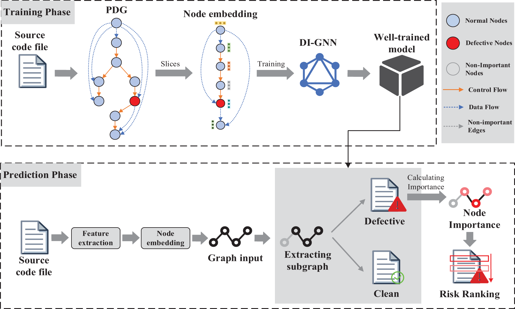
Figure 2: The framework of DIDP

3.1 Feature Extraction

We first extract the PDG corresponding to the source code file, which contains the data dependencies and control dependencies. The code example in Fig. 3 shows an example Java method snippet from ActiveMQ version 5.2.0 and the corresponding PDG, where the blue dashed arrow indicates the data flow of the “node” variable and the orange solid arrow indicates the control flow. The red box on Line 116 indicates the defective statement. Even though the logical exception is caught by adding try and catch statements in Lines 109 and 120–122, the code may affect other statements and thus introduce postrelease defects.

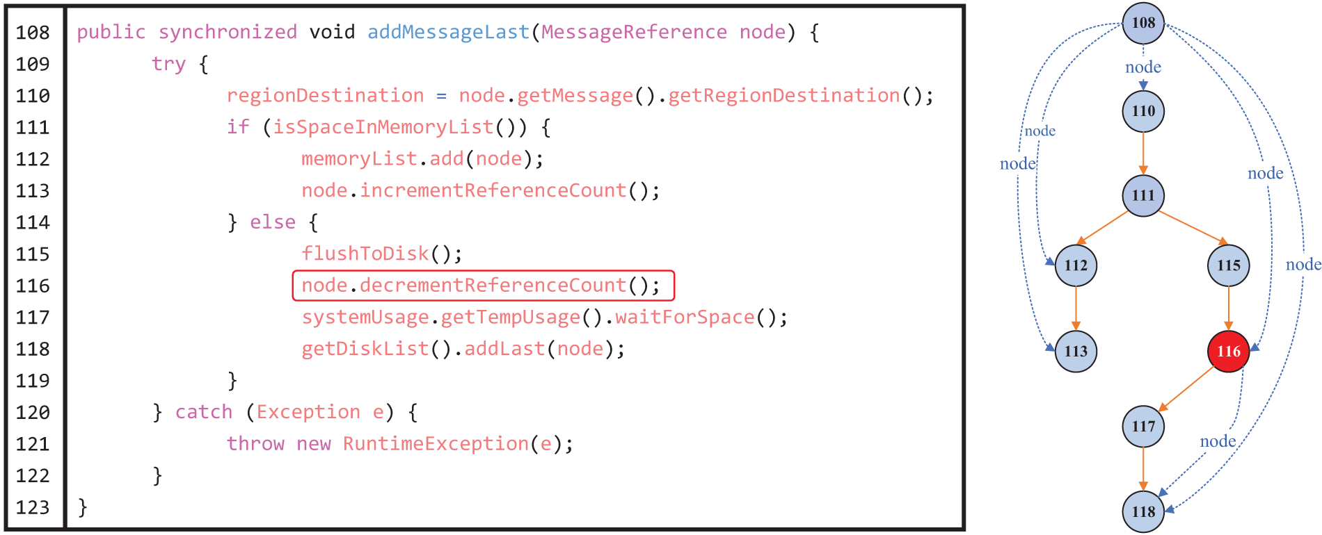
Figure 3: PDG for the “addMessageLast” module

However, while a file often contains tens or even hundreds of lines of code, defects are present in only a few of them. Therefore, simply using the entire source code file to train the model may reduce the ability of the model to identify key features. Therefore, based on the work of Cao et al. [28], we perform slicing operations on the whole PDG, i.e., backward and forward slicing starting from the defective nodes to avoid interference from irrelevant statements. Notably, we only perform slicing on the files in the training set and do not perform any operations on the test set. Specifically, we perform slicing operations on the PDG based on the code statements marked as defective in the dataset. As shown in Fig. 4, we perform backward slicing based on the presence of control dependencies or data dependencies with the defective statements, whereas we perform forward slicing based on data dependencies only, because forward control dependencies usually introduce many statements that are not related to that defective node. Owing to the problem of dataset labelling (the file-level dataset used in this paper does not have statement-level labels), in this paper, slicing operations are performed only on the dataset of the statement-level defect prediction experiments.

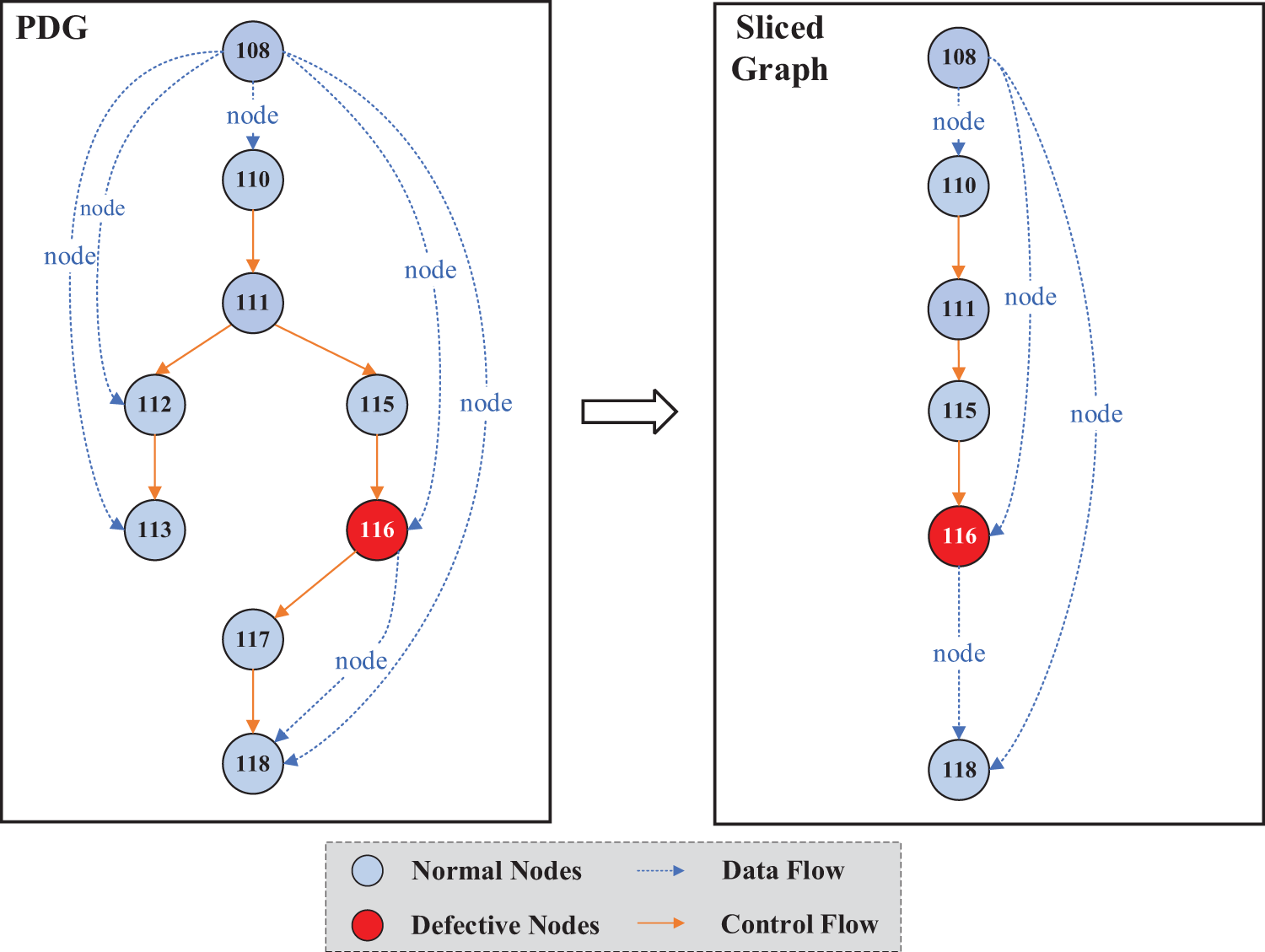
Figure 4: The PDG slicing example

The original PDG corresponding to the “addMessageLast” method and the corresponding sliced graph are shown in Fig. 4. The slicing operation is performed according to the defective Node 116, and since there is a backward control dependency between Node 115 and Node 116, Node 115 is reserved with the previous nodes that have a backward control dependency (Node 110 and Node 111). Node 108 has a backward data dependency with 116, and therefore it is also reserved.

Node 117 has only forward control dependency on Node 116, so that it is eliminated, and Nodes 112 and 113 are also eliminated due to their lack of direct dependency with Node 116. In the subsequent operation, we need to predict the sliced graph, and we write the sliced graph after the slicing operation as G=<V,E>, where V represents the node variable corresponding to the sliced graph G and E represents the edges in graph G corresponding to the control dependency or data dependency relationship. By adopting this method, we can conveniently perform prediction analysis on the sliced graph.

3.2 Node Embedding

After feature extraction, we convert all statements corresponding to nodes V in the sliced graph G into a low-dimensional space vector representation x and then use the graph G after node embedding as the input to the DI-GNN model.

Doc2vec [29] is an unsupervised technique for converting text to vectors that has been used and accepted by a wide range of researchers. Compared to other word embedding methods that crop excessively long tokens in the process of obtaining a fixed-length vector, Doc2vec can represent statement features more completely and accurately. Unlike Word2vec, which converts words into text, Doc2vec can convert arbitrary variable-length text into fixed-length vectors. Therefore, we use Doc2vec to convert the line of code into vector representations as node embeddings of graphs. Doc2vec learns the embeddings of paragraphs and files using the distributed memory model of paragraph vectors (PV-DM) and distributed bag-of-words model of paragraph vectors (PV-DBOW) to learn embeddings of paragraphs and files. These algorithms use hierarchical softmax or negative sampling. In the PV-DM model, each sentence is represented by a unique vector, which is represented by one of the columns of the matrix D. Each word is also represented by a unique vector, which is represented by one of the columns of the matrix W. Fixed length words are slide-sampled from one sentence at a time, and one of the words is taken as a predictor, while the others are used as input words. Each time a fixed length word is slide-sampled from a sentence, one of the words is taken as the predicted word, and the others are used as input words. The word vector corresponding to the input word and the sentence vector corresponding to this sentence, the paragraph vector, are input into the input layer, and the vector of this sentence and the sampled word vector are averaged or accumulated to form a new vector X. This vector X is then used to predict the predicted words in this window, and finally, the low-dimensional space vector X of the statement is obtained.

3.3 Graph Learning

After feature extraction, we convert all statements corresponding to nodes V in the sliced graph G into a low-dimensional space vector representation x and then use the graph G after node embedding as the input to the DI-GNN model.

We end up with a sliced graph G after node embedding to represent source code files; thus, we define the task of predicting file defects as a graph classification task. To effectively mitigate the impact of data drift, we build a novel graph learning framework, DI-GNN, to learn the graph. The key idea of DI-GNN is to learn the most relevant subgraph to exclude the features that are pseudocorrelated or irrelevant to the defects and then predict the results on the basis of the defect-relevant subgraph, thus making the model prediction immune to data drift. When implementing file-level predictions, it is important to understand which specific statements may be the cause of defects. Therefore, we need to further analyse which nodes in the graph contribute more to the defects. To reliably interpret file-level prediction, we introduce a novel attention method, namely the graph stochastic attention mechanism [15]. Existing work shows that the graph stochastic attention mechanism can provide a strong generalization capability together with highly reliable interpretation.

Graph stochastic attention mechanism principle: First, each edge E of graph G is given an intermediate attention weight, indicating the sampling probability of that edge in training. To encourage each edge to obtain a smaller sampling probability, i.e., to maintain a greater randomness, a regularization term must be introduced. However, if edges that are important for prediction results have high randomness, they are discarded too often during training, which greatly affects the classification loss (in our experiments, we calculate the classification loss in the form of cross-entropy). Thus, driven by classification loss, the important edges will eventually remain less random, i.e., obtain a larger sampling probability (ideally close to 1). Finally, the degree of randomness of each edge indicates its importance to the prediction performance; with important edges having a larger sampling probability. We consider the subgraph consisting of the edge with the largest sampling probability to be the most important subgraph, i.e., the subgraph most relevant to the label information. The nodes in this subgraph are the most relevant statements leading to defects.

Training objective: The method for selecting the regularization terms plays a key role in the above-described procedure. Since our goal is to control the randomness in the training graph, a reasonable and intuitive choice is to introduce the IB principle. By introducing the IB principle, we can control the amount of information in the graph to achieve the desired effect. Based on the method of Wu et al. [27] when selecting the subgraphs related to the labels by using information constraints, we define the optimization objective of subgraph identification as follows:

minθ,ϕ−I(fθ(Gs);Y)+βI(Gs;G),s.t.Gs∼gϕ(G)(1)

where Gs denotes the label-related subgraph, I(Gs;Y) denotes the mutual information (MI) between Gs and Y, and β is a canonical coefficient that controls the injection strength of the information bottleneck. gϕ is a model for extracting the label-related subgraph Gs from the original graph G, and fθ is a model for performing downstream task prediction on the extracted subgraph Gs. In our experiments, the parameters of gϕ and fθ are consistent except for in the last layer of the MLP. However, directly optimization of the amount of mutual information in Eq. (1) is very difficult. Separate variational upper bounds must be derived for two of the above objectives to optimize this objective.

For −I(fθ(Gs;Y)) in Eq. (1), we can easily obtain the variational upper bound as −EGS,Y[logPθ(Y|GS)], which represents the cross-entropy loss generated by fθ after prediction on the basis of the label-related subgraph Gs. For I(Gs;G) in Eq. (1), we can obtain its variational upper bound as E[KL(Pϕ(GS|G)||Q(GS))], where Pϕ(GS|G) is the sampling probability of each edge obtained by gϕ on the basis of G. Q(GS) is an edge distribution used to control the KL scatter term in the GIB objective, which can be considered as a prior distribution to specify the distribution of attention weights that we want the model to learn, because the KL scatter essentially encourages the sampling distribution of each edge obtained by learning to approximate the Q(GS) distribution. For example, if Q(GS) is a Bernoulli distribution with a parameter of 0.7, then this term will encourage the sampling probability of each edge to be close to 0.7, which aligns with how the regularization term is expected to act in the stochastic attention mechanism. The final training goal of the DI-GNN is classification loss (to accurately predict whether a file is defective), plus a regularization term for KL scatter (to encourage high randomness). Ideally, we want the training goal to be minimized when the model ensures small randomness only for the important edges. Thus, we obtain the highest overall randomness while achieving the highest classification performance. Through this approach, we are finally able to sample a subgraph that is most relevant to the defect information and that excludes features that are either pseudorelated or irrelevant to the defect.

DI-GNN model architecture: DI-GNN is divided into a subgraph extractor gϕ and a predictor fθ. gϕ accepts the sliced graph G as input and then outputs the random attention value of each edge. Then, based on the stochastic attention values, gϕ samples a label-related subgraph GS, and finally, GS is fed into the predictor fθ for defect prediction.

With the graph learning approach described above, DI-GNN can remove spurious correlations from the training data and achieves model interpretability while ensuring generalization performance. Thus, DIDP can achieve stable file-level prediction while identifying which statements are the key factors leading to defects.

3.4 Prediction Phase

In the prediction phase, we predict defects in the source code file using the trained DI-GNN and rank the risks of the different statements in the defect file. The graph learning process of DI-GNN and the risk ranking of the implemented statements are shown in Fig. 5.

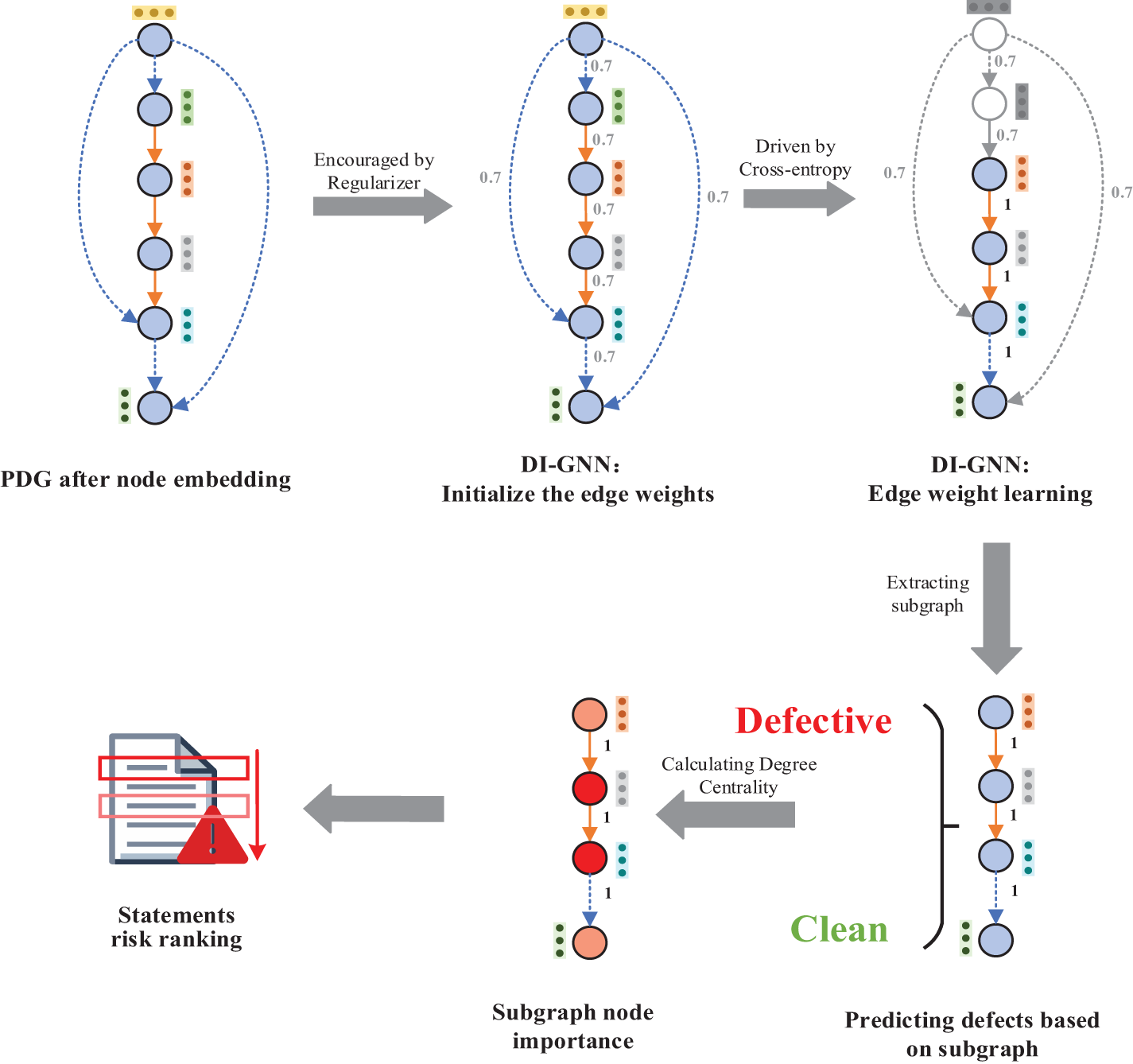
Figure 5: DI-GNN for graph learning and risk ranking of statements

Specifically, similar to the training phase, we first extract the PDG corresponding to the source code file. We further use Doc2vec to convert the statements corresponding to the nodes in the PDG into a low-dimensional space vector representation. Finally, unstructured information (low-dimensional space vectors obtained by Doc2vec conversion) and structured information (control dependency and data dependency relationships) are fed into DI-GNN as graphs for prediction. DI-GNN first extracts the predicted defect-related subgraph in the PDG and performs defect prediction on this predicted subgraph.

When defects are predicted to be present in the file, we further analyse the key statements that lead to defects in the file on the basis of the predicted label-related subgraph. The more important a line of code is, the more it contributes to the program semantics (i.e., functionality) of the implemented function [30]. Degree centrality [31] measures the percentage of nodes connected to the current node. It is the most direct metric for characterizing node centrality in network analysis; a greater degree of a node corresponds to a higher degree centrality and greater importance of the node in the network. Therefore, we introduce the degree centrality value to measure the node importance as a risk factor for statements in the defective file.

4  Experimental Design

Our experiments were conducted on a computer with an NVIDIA GTX 3060 GPU, i7-11700K 16-core CPU, running Ubuntu OS and using Python 3.8 as the programming language. The graph neural network was trained in batches until convergence, with a batch size of 128. The dimensionality of the vector representation of each node was 100, and the dropout was set to 0.1. We trained the model using the Adam [32] optimization algorithm with a learning rate of 0.001. The other hyperparameters of the neural network were tuned via grid search.

To validate the effectiveness of the DIDP approach, we propose the following two research questions and the corresponding experimental designs. To validate the effectiveness of the DIDP approach, we formulated two research questions along with the corresponding experimental designs. The first question examines whether DIDP is effective for file-level defect prediction, while the second question explores its effectiveness for statement-level defect prediction.

4.1 Research Questions

RQ1: What is the performance of DIDP on file-level defect prediction?

RQ2: How effective is DIDP in locating defective statements?

4.2 Experimental Datasets

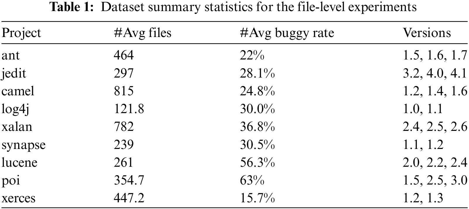
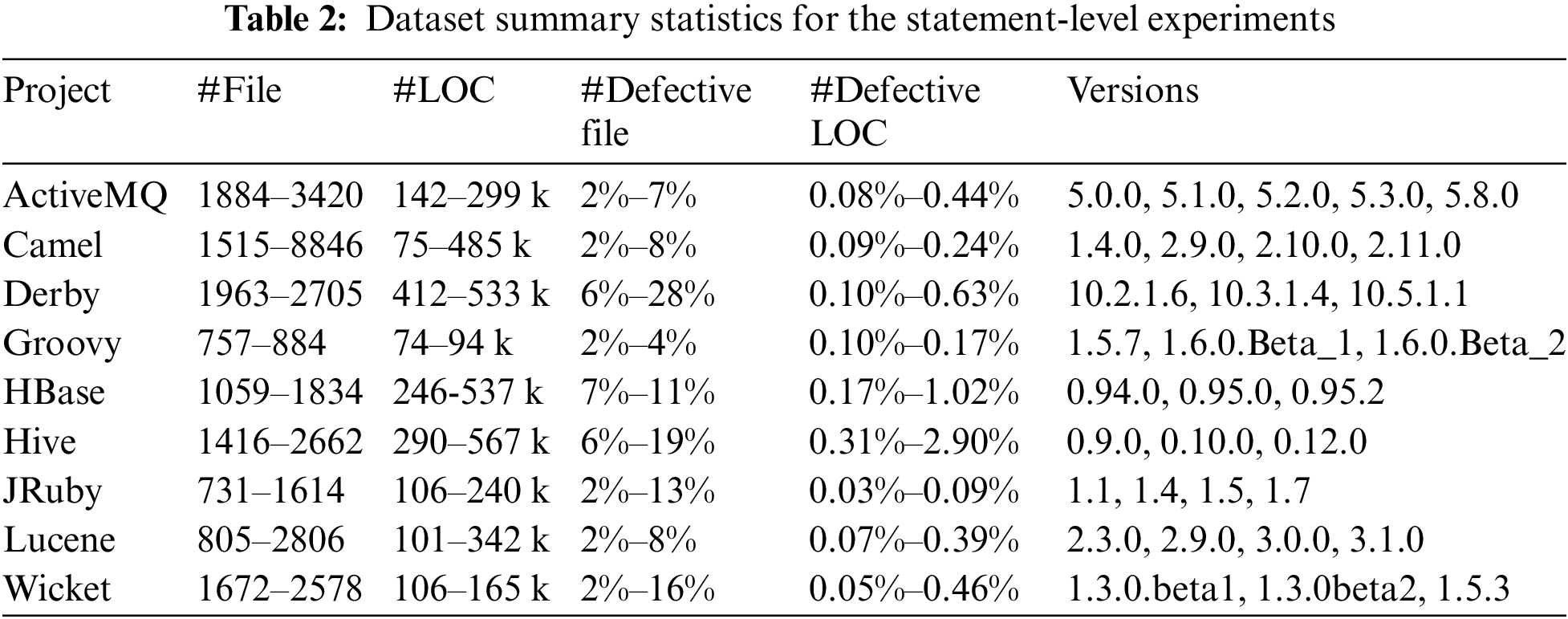
In this study, we used a publicly accessible dataset from the PROMISE repository to validate our file-level SDP experiments, specifically focusing on 9 Java projects selected from the PROMISE dataset [26]. For statement-level defect prediction, we utilized the benchmark dataset compiled by Wattanakriengkrai et al. [14], which comprises 32 versions of nine open-source software systems. Tables 1 and 2 provide brief statistical summaries of these datasets.

4.3 Evaluation Metrics

We evaluated the prediction performance of DIDP at the file-level using two traditional metrics that are widely used in the SDP domain; its cost-effectiveness for statement-level defect prediction was measured using three effort-aware evaluation metrics. The average prediction performance of the model was measured by the median [33].

(1) Metrics for the file-level experiments

The F1-score (F1) is the summed average of precision and recall, which combines precision and recall and can be used as a comprehensive index for model evaluation. It is calculated as follows:

F1−score=2∗Recall∗PrecisonRecall+Precision(2)

AUC: AUC serves as an evaluation metric in real-time SDP research, as reported in [28]. The receiver operating characteristic (ROC) curve is constructed by establishing various classification thresholds when assessing the performance of the model classifier. The ROC curve plots the false-positive rate (FPR) along the horizontal axis and the true positive rate (TPR) along the vertical axis. This curve is composed of coordinate points generated for each classification threshold, which represent the FPR and TPR values.

(2) Metrics for the statement-level experiments

Recall@Top20%LOC precisely measures how many defective statements can be found when examining the top 20% of statements throughout the release. Higher Recall@Top20%LOC values indicate that the method can rank many actual defective statements at the top. When the effort is fixed, more actual defective statements can be found; lower Recall@Top20%LOC values indicate that more nondefective statements are in the top 20% of statements and that developers must exert greater effort to locate defective statements.

Effort@Top20%Recall measures the amount of effort required to find the top 20% of actual defective statements in the entire release (e.g., LOC). Lower Effort@Top20%Recall values indicate that the top 20% of actual defective statements can be found with little effort on the part of the developer; thus, higher values of Effort@Top20%Recall indicated the need for greater effort to be exerted by the developers to find the actual defective statements in the top 20% of the entire release.

The initial false alarm (IFA) value is the number of nondefective statements that developers must check until the first defective statement is found for each file [34]. Lower IFA values indicate that there are fewer defective statements in the top ranking, while higher IFA values indicate that developers will need to spend more unnecessary effort on nondefective statements. This metric addresses the possibility that if developers cannot obtain promising results (i.e., find defective statements) in the first few lines of code inspection, they may stop subsequent inspections [35].

5  Analysis of Results

5.1 RQ1: What Is the Performance of DIDP on File-Level Defect Prediction?

To compare the effectiveness of our DIDP method on file-level prediction, we select ten state-of-the-art file-level SDP methods to evaluate the model prediction performance on two traditional evaluation metrics. In the WPDP experiments, the previous software version is employed for training and validation, whereas the subsequent version is used for prediction. For example, the model is trained using an earlier release of Xalan, specifically “xalan-2.4,” and then this trained model is utilized to predict defects in the next release, “xalan-2.5.” In the CPDP setting, the prediction model is initially trained on a project with ample labeled defect data. This trained model is subsequently applied to predict defects in a different project that has limited labeled data available [26].

①   Deep belief network (DBN) [19]: A defect prediction model with semantic features and source code change features generated by the DBN.

②   Deep transfer learning defect prediction (DTLDP) [22]: A framework for defect prediction that represents the source code file (or binary file) as images and extracts defect-related features using the AlexNet model.

③   Multi-flow graph neural network (MFGNN) [23]: A source code representation model that integrates the AST and the basic blocks of the CFG and then uses graph attention networks to learn features for defect prediction.

④   Augmented-code graph defect prediction (ACGDP) [24]: A graph-based code representation model that extracts code graph features, followed by the application of graph neural networks to acquire features and make predictions regarding software module defects.

⑤   Deep hierarchical convolutional neural network (DHCNN) [26]: As a graph-based deep learning approach, DHCNN combines abstract syntax tree, control flow graph and data dependence graph for software defect prediction using CNN models.

⑥   Bayesian networks (BN) [36]: A defect prediction model utilizing BN to reveal the probabilistic dependencies between software metrics and defect proneness.

⑦   CNN [37]: A defect prediction model that accepts ASTs as input to capture the semantic features of source code.

⑧   Semantic model (Seml) [38]: (word embedding + long short term memory (LSTM): A defect prediction model based on semantic word embedding and an LSTM network.

⑨   BugContext [39]: A bug detection approach that uses contextual dependencies from program dependence graphs and data flow graphs and then feeds them into the attention neural network.

⑩   LSTM [40]: An SDP framework using LSTM that extracts the syntactic features from ASTs of the program files and uses these features to predict defects.

We compared two metrics that are widely used in the SDP field and rank the methods in this paper as well as the baseline methods. We use the Wilcoxon signed rank test (WSRT) and Scott-Knott ESD (SK ESD) effect test [41,42] to determine whether the performance difference between the DIDP and the baseline model is statistically significant. “↑” indicates that the larger values of the metric correspond to better model performance. “↓” indicates that smaller values of the metric correspond to better model performance.

The WSRT constitutes a statistical hypothesis test that does not rely on any particular distributional assumption. It is utilized to evaluate whether two paired samples emanate from an identical distribution. A p-value resulting from the test that is less than 0.05 signifies a statistically significant difference between the matched samples; conversely, a p-value of 0.05 or greater does not imply a significant difference [25]. To mitigate the impact arising from multiple testing, the Win/Tie/Loss indicator is employed as a metric to assess the performance of various models. This methodology has been previously adopted in research studies to compare the efficacy of different methods, as reported previously [11].

To conduct a comprehensive multidimensional comparison between DIDP and other methods, we also employed the Scott-Knott effect size difference test method [33]. This approach leverages a hierarchical clustering algorithm to delineate clusters of means and assesses the statistical significance of disparities among these clusters. The detailed procedure is delineated as follows: 1) Optimal grouping identification: Initially, hierarchical clustering is utilized to ascertain the division that maximizes the mean value of the component measurements. This initial step facilitates the coherent grouping of samples exhibiting similar measurements, enabling a more precise comparison of their respective performances. 2) Grouping or merging process: After identifying the optimal grouping, specific combinations are either merged into a single group or a group is divided into two, on the basis of discernible differences among the samples. The objective of this step is to pinpoint notable discrepancies between the groups, ultimately allowing for the determination of the models that exhibit a statistically significant performance advantage.

(1) Within-Project Defect Prediction of File-Level Experiments

Tables 3 and 4 present the file-level AUC and F1-scores in WPDP obtained using both the proposed method and the comparison methods. In the experiment, DIDP exhibits robust predictive performance, as evidenced by competitive AUC and F1-scores across several projects. It consistently approaches or surpasses the benchmarks set by top performers such as ACGDP and DHCNN, particularly highlighted by its nearly equivalent median AUC and F1 values. The statistical significance of DIDP’s performance improvements is validated with p-values below 0.05, underscoring its superior efficacy relative to the eight compared methods. While ACGDP and DHCNN slightly outperform DIDP, possibly owing to their integration of abstract syntax tree structures alongside data and control flows, DIDP’s performance remains commendably high. Thus, DIDP stands out as a highly effective method in WPDP, suggesting that further enhancement can be achieved by incorporating additional structural analysis similar to that used in its top-performing counterparts.

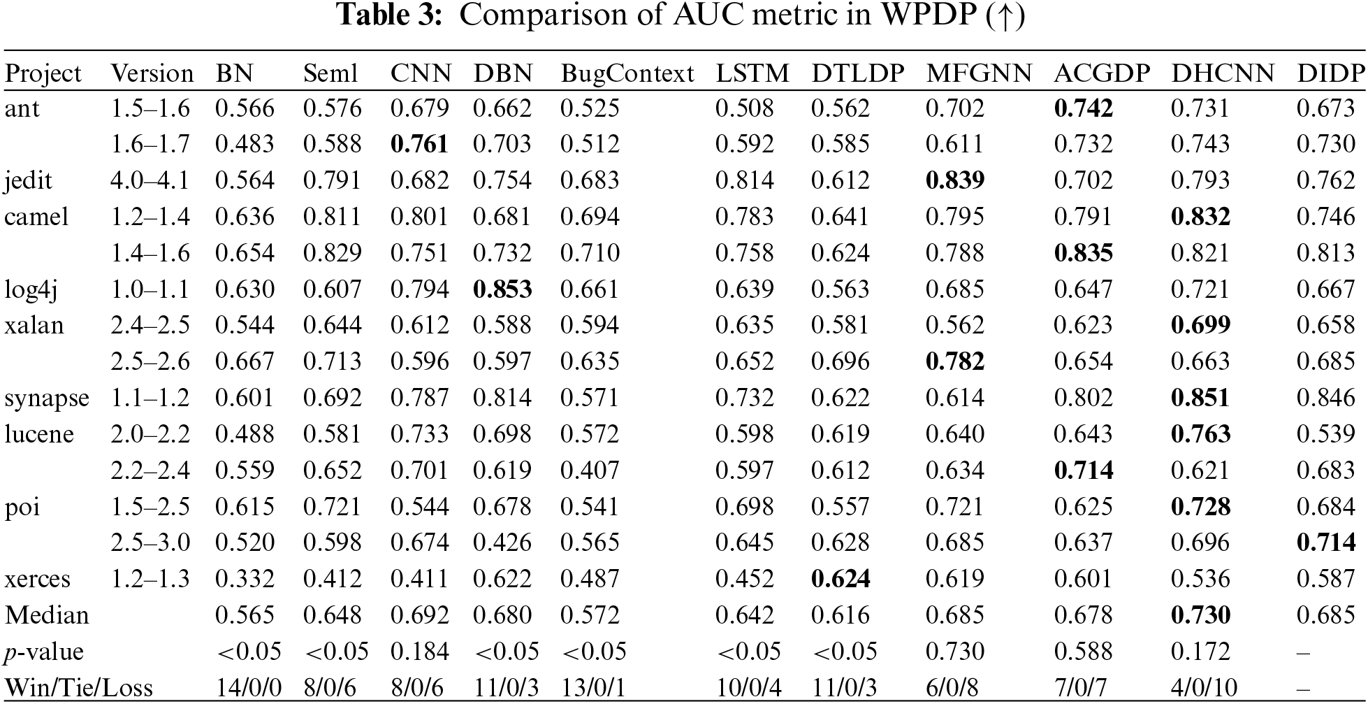
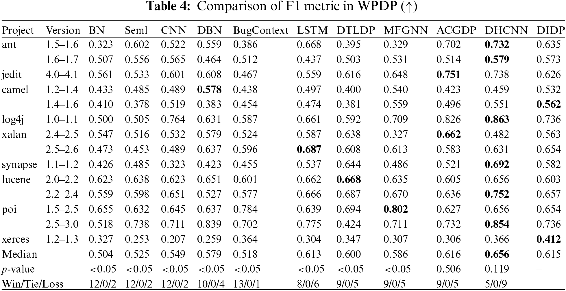
Fig. 6 shows the SK ESD test results for AUC and F1. The SK ESD test results offer a detailed comparative analysis of predictive models for WPDP, using both AUC and F1 metrics. While DHCNN shows the highest performance, our DIDP, which achieves an impressive second rank, is tied with ACGDP. As mentioned before, DHCNN and ACGDP incorporate abstract syntax trees, control flow graphs and data flow graphs and therefore achieve better results. However, DIDP is effective and closely approximates the top-performing DHCNN, demonstrating its robust ability to accurately predict software defects. The competitive performance of DIDP, particularly in comparison with the well-established models, highlights its potential for practical applications and further development. The strong performance of the method in terms of both the AUC and F1-score suggests that DIDP is not only statistically significant but also practically relevant in contexts where precise defect prediction is critical.

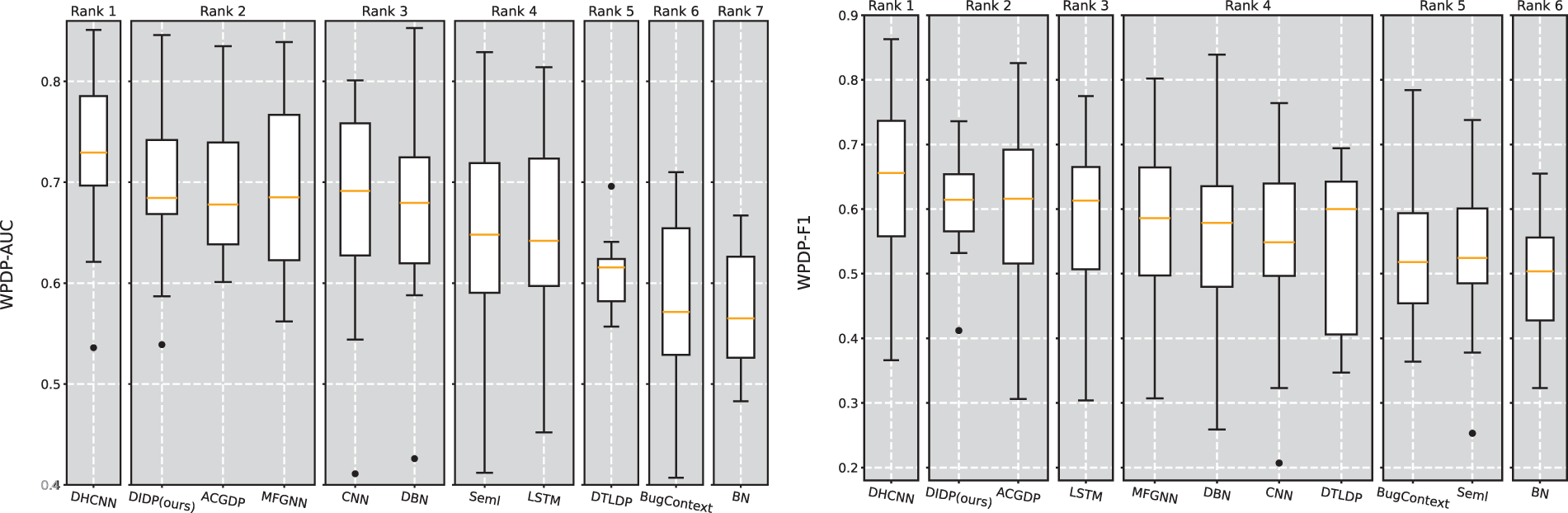
Figure 6: Scott-Knott effect size difference test for the AUC and F1 in WPDP

(2) Cross-Project Defect Prediction of File-Level Experiments

The results in Tables 5 and 6 show that DIDP achieves a median AUC of 0.651, which is just below that of DHCNN (0.658) and above those of most other comparison methods. This result indicates that DIDP has strong discriminative ability across diverse cross-project scenarios. Although DIDP does not surpass DHCNN in terms of the median AUC, its close performance (with a win/tie/loss ratio of 9/0/9 against DHCNN) highlights its effectiveness in accurately identifying defective modules across projects. Notably, DIDP’s p value of 0.766 against DHCNN in the Wilcoxon test suggests that the difference between the two models is not statistically significant, emphasizing DIDP’s competitiveness. For the F1 metric, DIDP achieves a median of 0.558, which is the highest among the models tested, underscoring its balanced performance in terms of precision and recall. This result is particularly valuable in defect prediction, where both false-positives and false-negatives must be minimized. The F1 performance of DIDP, with a win/tie/loss ratio of 10/0/8 against DHCNN, further supports its robustness in handling cross-project data.

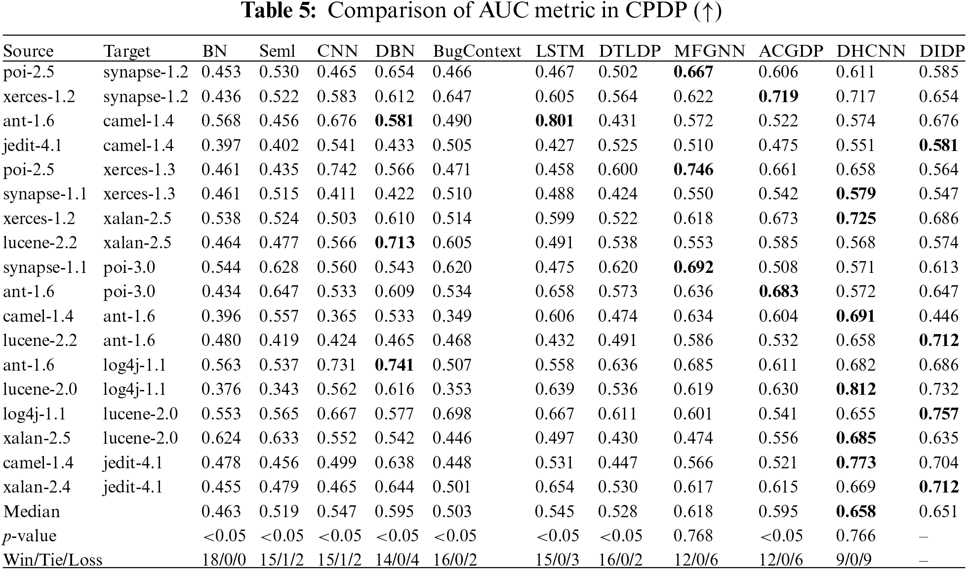
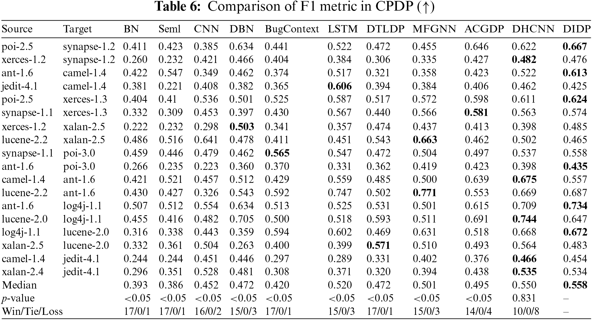
Fig. 7 shows the SK ESD test result for the AUC and F1 in CPDP. The experimental results show that DIDP achieves the same excellent performance as the current state-of-the-art DHCNN and outperforms ACGDP and MFGNN in CPDP. These results reveal that DIDP consistently shows high performance for both the AUC and F1 metrics, often matching or surpassing other models such as ACGDP and DHCNN. The lack of statistically significant differences between DIDP and the top-ranked models in many cases underscores DIDP’s practical utility and potential for further refinement. Given these findings, DIDP demonstrates reliable cross-project defect prediction capabilities, positioning it as a competitive and effective choice in CPDP applications.

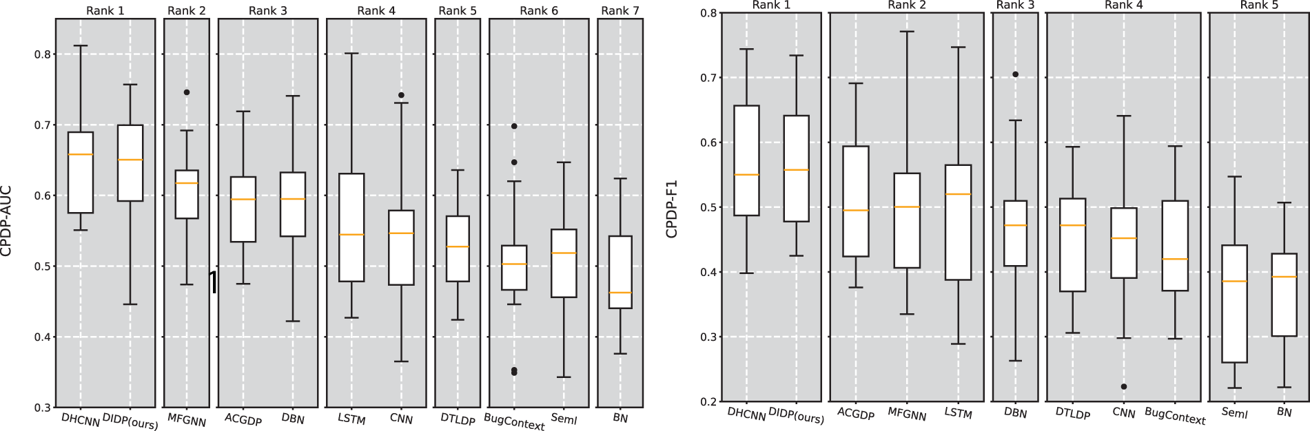
Figure 7: Scott-Knott effect size difference test for AUC and F1 in CPDP

Answer for RQ1: Our DIDP method shows strong predictive performance in both WPDP and CPDP tasks. In WPDP, DIDP achieves competitive AUC and F1-scores, ranking close to the leading methods such as DHCNN and ACGDP, as validated by the SK ESD test. In CPDP, DIDP maintains high accuracy, with a median AUC close to that of DHCNN and the highest F1-score among the models tested, reflecting a balanced approach to precision and recall. These findings confirm that DIDP is a competitive method for defect prediction across different project settings.

5.2 RQ2: How Effective Is DIDP in Locating Defective Statements?

(1) Within-Project Defect Prediction of Statement-Level Experiments

To validate the cost-effectiveness of DIDP in predicting the risk ranking of code statements, we select three state-of-the-art statement-level defect prediction methods and perform a comparative analysis on three effort-aware metrics.

The IVDetect [43] method extracts a key subgraph when interpreting a file defect; in this method, the corresponding nodes can be regarded as the key statements that lead to the existence of defects in the file. IVDetect does not implement statement-level risk ranking, but to compare our method with IVDetect, we also use degree centrality to calculate the risk factor for the corresponding statement in the key subgraph extracted by the IVDetect method (we denote the modified IVDetect method as IVDetect*). Moreover, we consider statements not present in the key subgraph as nondefective statements, thus achieving risk ranking of code statements.

LineVD [44] is a novel deep learning framework that specializes in statement-level vulnerability detection. LineVD treats statement-level vulnerability detection as a node classification task and uses GNN to capture control and data dependencies between statements.

ErrorProne [45] is a static analysis tool developed by Google. It is built on top of a rudimentary Java compiler (javac) and can check for defects in the source code against a set of Error-Prone rules. If a defect is generated by ErrorProne, the statement is considered defective. This detection emulates a top-down reading approach, where the developer examines the source code in order from the top to the bottom of the source code file.

Table 7 shows the results for DIDP compared with those for the other three baseline methods for statement-level defect prediction on the three effort-aware metrics. Fig. 8 shows the distributions of DIDP and the three baseline methods on the test set for the statement-level prediction results and the SK ESD effect test rankings. For Recall@Top20%LOC (Table 7), at the median, DIDP is 0.377, ErrorProne is 0.079, IVDetect* is 0.292, and LineVD is 0.308. Additionally, DIDP outperforms the four baseline methods on the majority of versions; as shown in Fig. 8a, it ranks first in the Scott-Knott ESD Effectiveness test, and the results of this experiment showed that DIDP was able to help testers find more defective statements when checking the first 20% of statements across the version. As shown by the experimental results in Table 7 and Fig. 8b, DIDP has the best median (0.175) on Effort@Top20%Recall and is tied for first place in the Scott-Knott ESD effect test. This shows that DIDP needs to check only 17.5% of the statements in the entire version to find the actual top 20% of the defective statements in the entire version, whereas ErrorProne, IVDetect*, and LineVD need to check 52.5%, 21.0%, and 19.5% of the code statements, respectively; thus DIDP requires the least amount of effort to find the actual top 20% of the defective code statements in the entire version. As shown by the experimental results in Table 8 and Fig. 8c, DIDP achieves the best median (69) in the IFA metric and ranks first in the SK ESD effect test, indicating that the risk ranking of the code statements generated by DIDP outperforms the other three baseline methods, so that developers using DIDP will spend less effort to find the first defective statement.

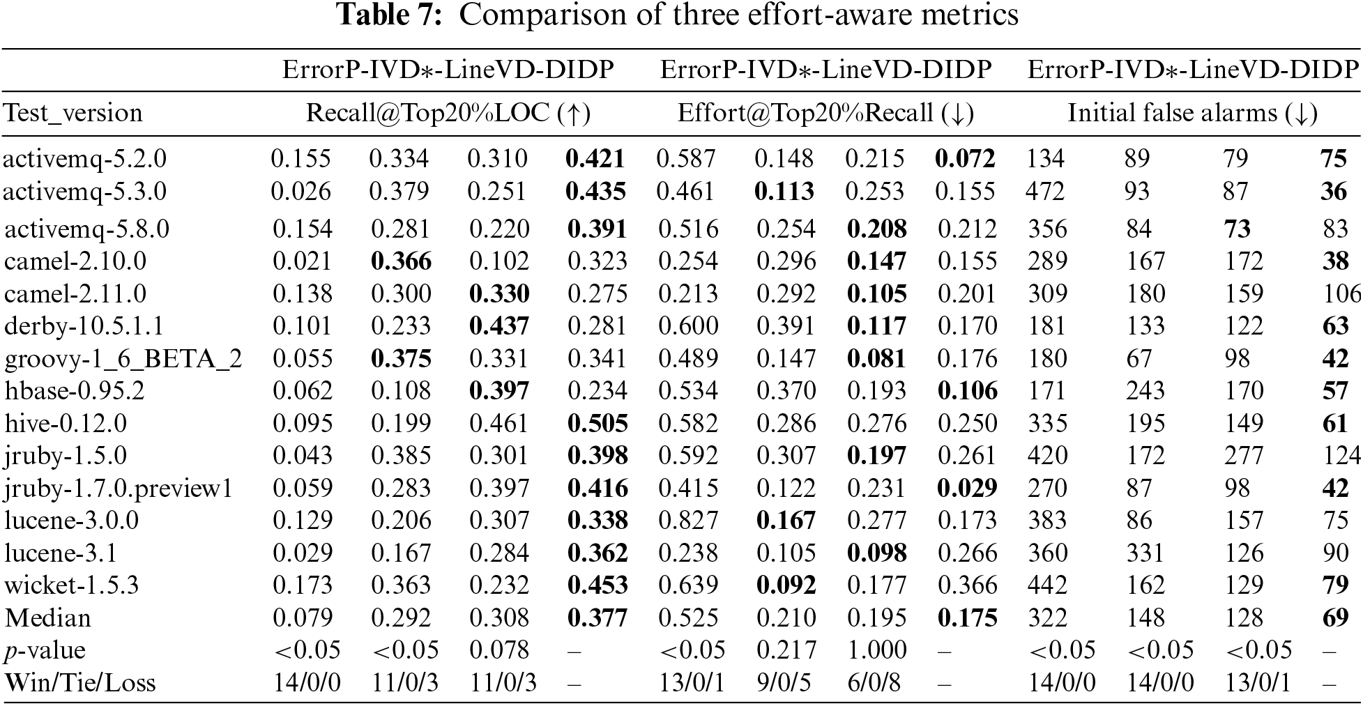
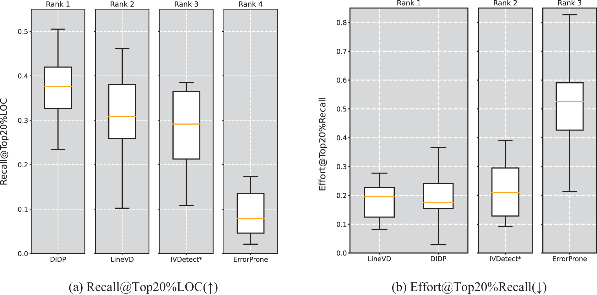
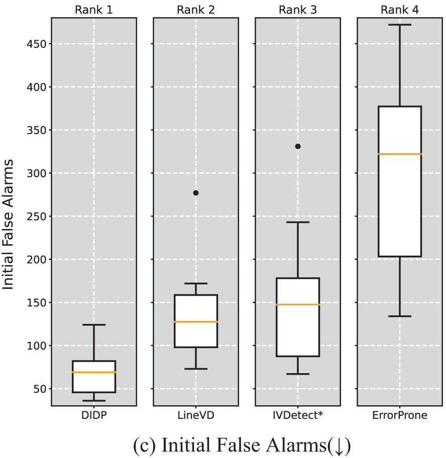
Figure 8: Scott-Knott effect size difference test for three effort-aware metrics

(2) Cross-Project Defect Prediction of Statement-Level Experiments

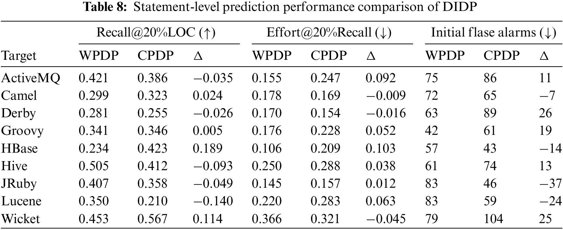
Since DIDP attempts to mitigate the model performance degradation caused by the training and test sets under different distributions at the model level, we further evaluate the prediction performance of DIDP at the statement-level in CPDP to explore whether DIDP can be applied to CPDP scenarios. Specifically, we use the first and second versions of the source project as the training and validation sets, respectively, and subsequent versions of the target project as the test set. Taking Camel as the target project, we use the first version of the other eight projects as the training set and the second version as the validation set to construct DI-GNN models for the eight different source projects. We predict the third and subsequent versions of the Camel project (i.e., Camel-2.10.0 and Camel-2.11.0) on each of these eight models and then take the median of the evaluation metrics on these two predicted versions as the average cross-project SDP prediction performance of DIDP on the Camel project. We then evaluate the cross-project prediction performance of DIDP at the statement-level using three effort-aware evaluation metrics. The experimental results of DIDP on statement-level cross-projects are shown in Table 8. We compare the performance of DIDP cross-version and cross-project predictions, where Δ denotes the performance difference between DIDP within and cross projects.

As shown by the experimental results in Table 8, for statement-level CPDP, our DIDP achieves 0.210–0.567 for Recall@Top20%LOC, 0.154–0.321 for Effort@Top20%Recall, and 43–104 for IFA. The experimental results in Table 8 show that when performing CPDP, DIDP can accurately locate 21.0%–56.7% of the actual defective statements when the top 20% of the code statements are checked. In addition, our DIDP method requires only 15.4%–32.1% of the LOC effort to find 20% efforts of the defective statements. DIDP requires 43–104 LOC effort to find the first defect. The above results show that DIDP may be more cost-effective when applied to WPDP, with a difference of −0.140 to +0.189 in Recall@Top20%LOC compared to WPDP. The CPDP prediction results for DIDP on some projects are even better than the WPDP results, and although the results may be worse on some projects, they are still within the acceptable range. In summary, DIDP achieves reasonable Recall@Top20%LOC, Effort@Top20%Recall, and IFA on cross-project statement-level SDP. The above results show that DIDP achieves the same excellent performance in CPDP as in WPDP.

Answer for RQ2: The experimental results demonstrate the cost-effectiveness of DIDP in statement-level defect prediction, in both the WPDP context and CPDP context. In WPDP, DIDP consistently outperforms baseline methods on effort-aware metrics, achieving the highest median Recall@Top20%LOC, Effort@Top20%Recall, and IFA scores. DIDP ranks first in the SK ESD tests across these metrics, indicating its ability to efficiently prioritize defective statements and minimize developer effort. For WPDP, DIDP achieves a Recall@Top20%LOC between 21.0% and 56.7%, an Effort@Top20%Recall between 15.4% and 32.1%, and an IFA ranging from 43 to 104. These results suggest that DIDP maintains high predictive accuracy and cost-efficiency in CPDP, with performance comparable to or exceeding that of WPDP in some projects. Overall, DIDP demonstrates strong adaptability and effectiveness in cross-project scenarios, supporting its applicability in diverse statement-level defect prediction tasks.

6  Discussion

(1) Why DIDP effectively mitigates data distribution differences

To address the data drift problem in SDP, we propose an SDP method named “DIDP”, which uses the graph stochastic attention mechanism to achieve guaranteed interpretability and generalization capability by injecting randomness into the learning of attention. The basic principle of this model stems from the concept of an information bottleneck, which aims to find an optimal data representation that enables it to retain as much defect-related information as possible while excluding as much defect-irrelevant information as possible. In this way, DI-GNN can mine the most critical features related to defects from software projects (since we use graph structure data to represent the source code, the most critical features correspond to the most relevant subgraph in the graph), thus alleviating data drift due to project development to a certain extent and improving the generalization performance of the model.

(2) DIDP vs. Static Analysis Tool

Static analysis tools (e.g., ErrorProne) rely heavily on well-defined defect rules or patterns that are handcrafted by domain experts, requiring considerable time and effort. At the same time, real-world software is large, and defects in this software are more complex. These issues limit the effectiveness of static analysis-based detectors. However, DIDP can automatically learn defect-related features hidden in software source code, i.e., structured (graph structure) and unstructured (semantic) information corresponding to source code, with only a small amount of a priori knowledge (i.e., labels of defective files and corresponding statements) needed to achieve highly accurate file-level and statement-level defect prediction. Therefore, DIDP can automatically learn defect-related features hidden in software source code with higher accuracy than static analysis tools. In practical applications, DIDP and static analysis tools are not mutually exclusive, and they can complement each other to improve defect repair efficiency.

(3) DIDP vs. Deep Learning Methods

Among the many deep learning approaches related to SDP, researchers have proposed various source code characterization methods to extract key defect features and have constructed many different DL models to improve model performance. However, these methods rarely consider the data drift problem during software development and fine-grained prediction. Some datasets have long release times between versions, with significant variations in the functionality and complexity between these versions. Therefore, the performance of the model may be significantly reduced when these methods are applied to datasets with long span times. By contrast, in cross-project SDP, a widely adopted approach is to select target project data with similar distributions to those of to the source project via migration learning because of the differences in data distributions between the source and target projects. In this paper, we introduce information bottleneck theory and a graph stochastic attention mechanism that predicts defects by learning the subgraph most relevant to the labels and filtering factors unrelated to the defects. This results in a novel defect prediction method that is robust to data drift. Moreover, we treat the statements corresponding to the relevant subgraph as risk statements and use degree centrality to calculate the importance of nodes, thus achieving fine-grained defect prediction. Therefore, compared with previous deep learning-based SDP methods, DIDP accounts for the degradation of model performance due to data drift problems, and can maintain excellent prediction results on datasets spanning a long time period. Additionally, DIDP achieves fine-grained defect prediction, which can effectively help testers quickly respond to high-risk statements that may lead to defects, thus improving defect repair efficiency.

7  Threats to Validity

7.1 Threats to Internal Validity

(1) The dataset labels we use are obtained via manual statistics, which means that labelling a dataset is a large and tedious task. As a result, some samples may be mislabelled during the labelling process. Nevertheless, since many studies have used the labelled datasets, their annotation results are still considered reliable.

(2) At the same time, an unavoidable problem in implementing the baseline method we used for comparison is that different programming environments and model parameters can impact the final results. To minimize this impact, we try to follow the approach presented in the baseline paper and the open-source code provided by the researchers for experimental replication.

7.2 Threats to External Validity

(1) We verify the effectiveness of DIDP on two SDP datasets. However, since the representation of source code in graph form is affected by various factors (e.g., code complexity, different application scenarios.), these results may not be satisfactory in practical applications. Additionally, we only carried out experiments on Java projects, so that the results may not be fully reproducible for other programming languages. However, since PDG is a graphical representation of a general language, DI-GNN can be applied to other languages to extract the corresponding key features. Therefore, it is also feasible to apply DIDP to other programming languages.

(2) In addition, since DIDP is specifically designed for release-based defect prediction models, it is not applicable to other types of defect prediction models (such as just-in-time defect prediction) because the structural information contained is inconsistent.

7.3 Threats to Construct Validity

Data drift is an inevitable problem during software updates, and it is not realistic to expect a model to achieve high-performance predictions in all subsequent versions of a given software. Although DIDP alleviates data drift to some extent, we still recommend updating the model to maintain its excellent prediction performance when it degrades significantly.

8  Conclusion

In this paper, we propose a novel defect prediction method, DIDP, for the data drift problem in software projects and construct a DI-GNN model that is robust to data drift by using concepts based on information bottleneck theory and a stochastic attention mechanism to embed both unstructured and structured information of source code statements, so as to more fully use the semantic and structural information of the source code to mine important features related to defects in the source code. Experimental results on two datasets show that our DIDP has better prediction performance than the state-of-the-art file-level methods and is more cost-effective than three fine-grained SDP methods. Although the median performance of DIDP is lower than that of ACGDP [24] and DHCNN [26] in within-project file-level prediction, we attribute this to the fact that both methods incorporate AST information, capturing the semantic structure of the program, and thereby achieving better prediction performance. However, in cross-project prediction, our method consistently ranks first in the SK ESD test, indicating that DIDP effectively mitigates the distribution differences between different projects.

In future research, we will also consider leveraging the strengths of existing methods to extract semantic information from programs (such as AST) to achieve better prediction performance. In addition, we plan to enhance our framework by integrating insights from recent advances in graph contrastive learning, such as those reported in recent studies [46,47]. These studies highlight the importance of leveraging contextual relationships and adaptive mechanisms, which we believe can further optimize contrastive learning approach within graph structures, leading to improved performance and robustness in our prediction tasks.

Acknowledgement: The authors would like to express appreciation to the National Natural Science Foundation of China (Grant No. 61762067) for their financial support.

Funding Statement: This research was supported by the National Natural Science Foundation of China (Grant No. 61762067).

Author Contributions: The authors confirm contribution to the paper as follows: study conception and design: Fengyu Yang, Fa Zhong, Xiaohui Wei, Guangdong Zeng; data collection: Fengyu Yang, Fa Zhong, Xiaohui Wei, Guangdong Zeng; analysis and interpretation of results: Fengyu Yang, Fa Zhong, Xiaohui Wei, Guangdong Zeng; draft manuscript preparation: Fa Zhong, Fengyu Yang. All authors reviewed the results and approved the final version of the manuscript.

Availability of Data and Materials: The data that support the findings of this study are openly at: https://github.com/awsm-research/line-level-defect-prediction (accessed on 14 November 2024).

Ethics Approval: Not applicable.

Conflicts of Interest: The authors declare no conflicts of interest to report regarding the present study.

References

1. L. N. Gong, S. J. Jiang, and L. Jiang, “Research progress of software defect prediction,” (in ChineseJ. Softw., vol. 30, no. 10, pp. 3090–3114, Aug. 2019. [Google Scholar]

2. N. Nagappan and T. Ball, “Static analysis tools as early indicators of pre-release defect density,” presented at the 27th Int. Conf. Softw. Eng., St. Louis, MO, USA, May 15–21, 2005. [Google Scholar]

3. Y. Nong, H. Cai, P. Ye, L. Li, and F. Chen, “Evaluating and comparing memory error vulnerability detectors,” Inf. Softw. Technol., vol. 137, no. 8, Sep. 2021, Art. no. 106614. doi: 10.1016/j.infsof.2021.106614. [Google Scholar] [CrossRef]

4. D. R. Ibrahim, R. Ghnemat, and A. Hudaib, “Software defect prediction using feature selection and random forest algorithm,” presented at the 2017 Int. Conf. New Trends Comput. Sci., Amman, Jordan, Oct. 252–257, 2017. [Google Scholar]

5. D. Gray, D. Bowes, N. Davey, Y. Sun, and B. Christianson, “Using the support vector machine as a classification method for software defect prediction with static code metrics,” presented at the 2009 11th Int. Conf. Eng. Appl. Neural Networks (EANNLondon, UK, Aug. 2009. doi: 10.1007/978-3-642-03969-0. [Google Scholar] [CrossRef]

6. L. Qiao, X. Li, Q. Umer, and P. Guo, “Deep learning based software defect prediction,” Neurocomputing, vol. 385, no. 2, pp. 100–110, Apr. 2020. doi: 10.1016/j.neucom.2019.11.067. [Google Scholar] [CrossRef]

7. S. Wang, J. Wang, J. Nam, and N. Nagappan, “Continuous software bug prediction,” presented at the 2021 15th ACM/IEEE Int. Symp. Empirical Softw. Eng. Meas., Bari, Italy, Oct. 1–12, 2021. [Google Scholar]

8. G. G. Cabral, L. L. Minku, E. Shihab, and S. Mujahid, “Class imbalance evolution and verification latency in just-in-time software defect prediction,” presented at the 2019 41st Int. Conf. Softw. Eng., Montreal, QC, Canada, May 2019, pp. 666–676. [Google Scholar]

9. Y. Kamei, S. Matsumoto, A. Monden, K. Matsumoto, B. Adams and A. E. Hassan, “Revisiting common bug prediction findings using effort-aware models,” presented at the 2010 IEEE Int. Conf. Softw. Maint., Timisoara, Romania, Sep. 1–10, 2010. [Google Scholar]

10. M. Yan, Y. Fang, D. Lo, X. Xia, and X. Zhang, “File-level defect prediction: Unsupervised vs. supervised models,” presented at the 2017 ACM/IEEE Int. Symp. Empirical Softw. Eng. Meas. (ESEMToronto, ON, Canada, Nov. 2017, pp. 344–353. [Google Scholar]

11. H. Wang, W. Zhuang, and X. Zhang, “Software defect prediction based on gated hierarchical LSTMs,” IEEE Trans. Rel., vol. 70, no. 2, pp. 711–727, Jan. 2021. doi: 10.1109/TR.2020.3047396. [Google Scholar] [CrossRef]

12. E. A. Felix and S. P. Lee, “Predicting the number of defects in a new software version,” PLoS One, vol. 15, no. 3, Jul. 2020, Art. no. e0229131. [Google Scholar]

13. C. Pornprasit and C. K. Tantithamthavorn, “JITLine: A simpler, better, faster, finer-grained just-in-time defect prediction,” presented at the 2021 IEEE/ACM 18th Int. Conf. Min. Softw. Repos., Madrid, Spain, May 2021, pp. 369–379. [Google Scholar]

14. S. Wattanakriengkrai, P. Thongtanunam, C. Tantithamthavorn, H. Hata, and K. Matsumoto, “Predicting defective lines using a model-agnostic technique,” IEEE Trans. Softw. Eng., vol. 48, no. 5, pp. 1480–1496, Sep. 2020. doi: 10.1109/TSE.2020.3023177. [Google Scholar] [CrossRef]

15. S. Miao, M. Liu, and P. Li, “Interpretable and generalizable graph learning via stochastic attention mechanism,” presented at the 2022 Int. Conf. Mach. Learn., Baltimore, MD, USA, Jul. 2022, pp. 15524–15543. [Google Scholar]

16. N. Tishby, F. C. Pereira, and W. Bialek, “The information bottleneck method,” 2000, arXiv:0004057. [Google Scholar]

17. N. Tishby and N. Zaslavsky, “Deep learning and the information bottleneck principle,” presented at the 2015 IEEE Inf. Theory Workshop, Jerusalem, Israel, Apr. 1–5, 2015. [Google Scholar]

18. D. Di Nucci, F. Palomba, G. D. Rosa, G. Bavota, and A. Lucia, “A developer centered bug prediction model,” IEEE Trans. Softw. Eng., vol. 44, no. 1, pp. 5–24, Jan. 2017. doi: 10.1109/TSE.2017.2659747. [Google Scholar] [CrossRef]

19. S. Wang, T. Liu, J. Nam, and L. Tan, “Deep semantic feature learning for software defect prediction,” IEEE Trans. Softw. Eng., vol. 46, no. 12, pp. 1267–1293, Oct. 2018. doi: 10.1109/TSE.2018.2877612. [Google Scholar] [CrossRef]

20. S. Ackerman, O. Raz, M. Zalmanovici, and A. Zlotnick, “Automatically detecting data drift in machine learning classifiers,” 2021, arXiv:2111.05672. [Google Scholar]

21. S. Amasaki, “On applicability of cross-project defect prediction method for multi-versions projects,” presented at the 2017 13th Int. Conf. Predict. Models Data Anal. Softw. Eng., Toronto, ON, Canada, Sep. 2017, pp. 93–96. [Google Scholar]

22. J. Chen et al., “Software visualization and deep transfer learning for effective software defect prediction,” presented at the 2020 ACM/IEEE 42nd Int. Conf. Softw. Eng., Seoul, Republic of Korea, Jul. 2020, pp. 578–589. [Google Scholar]

23. Z. Zhao, B. Yang, G. Li, H. Liu, and Z. Jin, “Precise learning of source code contextual semantics via hierarchical dependence structure and graph attention networks,” J. Syst. Softw., vol. 184, no. 1, Feb. 2021, Art. no. 111108. doi: 10.1016/j.jss.2021.111108. [Google Scholar] [CrossRef]

24. J. Xu, J. Ai, J. Liu, and T. Shi, “ACGDP: An augmented code graph-based system for software defect prediction,” IEEE Trans. Rel., vol. 71, no. 2, pp. 850–864, Apr. 2022. doi: 10.1109/TR.2022.3161581. [Google Scholar] [CrossRef]

25. A. Abdu, Z. Zhai, H. A. Abdo, R. Algabri, and S. Lee, “Graph-based feature learning for cross-project software defect prediction,” Comput. Mater. Contin., vol. 77, no. 1, pp. 161–180, Oct. 2023. doi: 10.32604/cmc.2023.043680. [Google Scholar] [CrossRef]

26. A. Abdu, Z. Zhai, H. A. Abdo, and R. Algabri, “Software defect prediction based on deep representation learning of source code from contextual syntax and semantic graph,” IEEE Trans. Rel., vol. 73, no. 2, pp. 1–15, Feb. 2024. doi: 10.1109/TR.2024.3354965. [Google Scholar] [CrossRef]

27. T. Wu, H. Ren, P. Li, and J. Leskovec, “Graph information bottleneck,” presented at the 2020 Adv. Neural Inf. Process. Syst., Vancouver, BC, Canada, Dec. 6–12, 2020. [Google Scholar]

28. S. Cao, X. Sun, L. Bo, R. Wu, B. Li and C. Tao, “MVD: Memory-related vulnerability detection based on flow-sensitive graph neural networks,” presented at the 44th Int. Conf. Softw. Eng., Pittsburgh, PA, USA, May 2022, pp. 1456–1468. [Google Scholar]

29. Q. Le and T. Mikolov, “Distributed representations of sentences and documents,” presented at the Int. Conf. Mach. Learn., Beijing, China, Jun. 2014, pp. 1188–1196. [Google Scholar]

30. Y. Wu, D. Zou, S. Dou, W. Yang, D. Xu and H. Jin, “VulCNN: An image-inspired scalable vulnerability detection system,” presented at the 44th Int. Conf. Softw. Eng., Pittsburgh, PA, USA, May 2022, pp. 2365–2376. [Google Scholar]

31. L. C. Freeman, “Centrality in social networks: Conceptual clarification,” Social Netw. Crit. Concepts Sociol., vol. 1, pp. 238–263, Oct. 2002. [Google Scholar]

32. D. P. Kingma and J. Ba, “Adam: A method for stochastic optimization,” presented at the 2015 3rd Int. Conf. Learn. Represent., San Diego, CA, USA, May 7–9, 2015. [Google Scholar]

33. C. Pornprasit and C. K. Tantithamthavorn, “DeeplineDP: Towards a deep learning approach for line-level defect prediction,” IEEE Trans. Softw. Eng., vol. 49, no. 1, pp. 84–98, Jan. 2022. doi: 10.1109/TSE.2022.3144348. [Google Scholar] [CrossRef]

34. Q. Huang, X. Xia, and D. Lo, “Supervised vs unsupervised models: A holistic look at effort-aware just-in-time defect prediction,” presented at the 2017 IEEE Int. Conf. Softw. Maint. Evol., Shanghai, China, Sep. 2017, pp. 159–170. [Google Scholar]

35. C. Parnin and A. Orso, “Are automated debugging techniques actually helping programmers?” presented at the 2011 Int. Symp. Softw. Test. Anal., Toronto, ON, Canada, Jul. 2011, pp. 199–209. [Google Scholar]

36. A. Okutan and O. T. Yildiz, “Software defect prediction using Bayesian networks,” Empir. Softw. Eng., vol. 19, no. 1, pp. 154–181, Aug. 2012. doi: 10.1007/s10664-012-9218-8. [Google Scholar] [CrossRef]

37. J. Li, P. He, J. Zhu, and M. R. Lyu, “Software defect prediction via convolutional neural network,” presented at the 2017 IEEE Int. Conf. Softw. Qual. Rel. Secur., Prague, Czech Republic, Jul. 2017, pp. 318–328. [Google Scholar]

38. H. Liang, Y. Yu, L. Jiang, and Z. Xie, “Seml: A semantic LSTM model for software defect prediction,” IEEE Access, vol. 7, pp. 83812–83824, Jun. 2019. doi: 10.1109/ACCESS.2019.2925313. [Google Scholar] [CrossRef]

39. Y. Li, S. Wang, T. N. Nguyen, and S. V. Nguyen, “Improving bug detection via context-based code representation learning and attention-based neural networks,” presented at the 2019 ACM on Program. Lang., Athens, Greece, 2019, vol. 3, no. OOPSLA, pp. 1–30. [Google Scholar]

40. J. Deng, L. Lu, and S. Qiu, “Software defect prediction via LSTM,” IET Softw., vol. 14, no. 4, pp. 443–450, May 2020. doi: 10.1049/iet-sen.2019.0149. [Google Scholar] [CrossRef]

41. C. Tantithamthavorn, S. McIntosh, A. E. Hassan, and K. Matsumoto, “The impact of automated parameter optimization on defect prediction models,” IEEE Trans. Softw. Eng., vol. 45, no. 7, pp. 683–711, Jan. 2018. doi: 10.1109/TSE.2018.2794977. [Google Scholar] [CrossRef]

42. C. Tantithamthavorn, S. McIntosh, A. E. Hassan, and K. Matsumoto, “Automated parameter optimization of classification techniques for defect prediction models,” presented at the 2016 38th Int. Conf. Softw. Eng., Austin, TX, USA, May 2016, pp. 321–332. [Google Scholar]

43. Y. Li, S. Wang, and T. N. Nguyen, “Vulnerability detection with fine-grained interpretations,” presented at the 2021 29th ACM Joint Meet. Eur. Softw. Eng. Conf. Symp. Found. Softw. Eng., Athens, Greece, Aug. 2021, pp. 292–303. [Google Scholar]

44. D. Hin, A. Kan, H. Chen, and M. Babar, “LineVD: Statement-level vulnerability detection using graph neural networks,” presented at the 2022 19th Int. Conf. Min. Softw. Repos., Pittsburgh, PA, USA, May 2022, pp. 596–607. [Google Scholar]

45. E. Aftandilian, R. Sauciuc, S. Priya, and S. Krishnan, “Building useful program analysis tools using an extensible java compiler,” presented at the 2012 IEEE 12th Int. Working Conf. Source Code Anal. Manipul., Riva del Garda, Italy, Sep. 14–23, 2012. [Google Scholar]

46. W. He, G. Sun, J. Lu, and X. S. Fang, “Candidate-aware graph contrastive learning for recommendation,” presented at the 2023 46th Int. ACM SIGIR Conf. Res. Dev. Inf. Retr., Taipei, Taiwan, Jul. 2023, pp. 1670–1679. [Google Scholar]

47. Y. Jiang, C. Huang, and L. Huang, “Adaptive graph contrastive learning for recommendation,” presented at the 2023 29th ACM SIGKDD Conf. Knowl. Discov. Data Min., Long Beach, CA, USA, Aug. 2023, pp. 4252–4261. [Google Scholar]