Study on Sediment Removal Method of Reservoir Based on Double Branch Convolution

1  Introduction

Among the various human endeavors to reshape the natural environment, one of the most grandiose and far-reaching projects is undoubtedly the construction of reservoirs by damming rivers. These reservoirs not only reconfigure the surface water systems but also profoundly alter the natural ecology and socio-economic landscapes. However, among the many challenges, the issue of sedi-mentation in reservoirs stands out, particularly for those built on rivers with high sediment loads. As these reservoirs are established, the water level is artificially raised, leading to the deposition of up-stream sediments within the reservoir area, resulting in severe siltation. This situation not only ac-celerates the reduction in reservoir capacity, shortening its expected lifespan, but also poses a direct threat to the safety of the dam. Confronted with this pressing issue, finding effective solutions has become an urgent task before us.

In recent years, the rapid development of sensor and communication technologies has made it possible to generate and record large amounts of continuous time-series data. Predicting long-term reservoir sediment discharge is a complex problem involving high dimensions [1], extended timeframes, and multiple stages [2]. The core of sediment discharge prediction involves detecting patterns in historical time-series data to anticipate future trends, which is critical for improving reservoir management strategies [3]. Accurate predictions assist in optimizing dam operations and sediment management strategies. Such as dam operation and reservoir sediment management [4].

In the field of sediment and water flow prediction, neural networks have made significant strides. Researchers have continuously refined sediment prediction models to improve their accuracy. For instance,. Similarly, Nagy et al. [5] integrated artificial neural networks with fluid dynamics and sediment transport principles, selecting hydrological and sediment variables that significantly impact model performance. They trained the model using field-collected data and validated its accuracy and generalization capabilities through comparisons with data from other rivers. AlDahoul et al. [6] used the Long Short Tern Memory (LSTM) algorithm to predict suspended sediment in the Johor River in Malaysia, aiming to solve the problem of low accuracy in traditional river runoff and sediment content prediction methods. This prediction method can predict daily, weekly, and monthly regression scenarios. Despite LSTM’s effectiveness as an optimized Recurrent Neural Network (RNN) for handling time-series data, RNN-based methods encounter difficulties with long time windows due to vanishing gradients, which increases computational cost and limits predictive accuracy over extended periods [7]. In recent years, there has been a notable shift in the technological landscape of time-series prediction, with more researchers gravitating towards Transformer-based methods [8], Convolutional Neural Networks (CNNs) [9], and simpler models like Multi-Layer Perceptrons (MLPs) [10]. However, the self-attention mechanism in Transformers exhibits permutation invariance, meaning it cannot inherently account for the original sequence order, potentially leading to the loss of critical temporal information. While Transformers offer a powerful tool for time-series modeling, they also introduce new challenges that must be addressed to ensure the proper capture and preservation of time dependencies.

In the application of hybrid models, Afan et al. [11] applied two distinct Artificial Neural Network (ANN) algorithms to improve the model’s capacity to predict daily sediment load by capturing different types of relationships in the data. By training and testing the models using daily sediment and flow data from the Lembangang Station on the Johor River, they were able to create an accurate sediment prediction model by combining flow and sediment data. In terms of deep learning applications, Ma et al. [12] used a neural network consisting of two branches. This includes an LSTM branch and a CNN branch. The LSTM branch is used to learn gas containing features in one-dimensional time series data, while the CNN branch is used to learn gas containing features in two-dimensional time series data. Finally, the outputs of the two branches are fused and the final prediction is made through the output layer. Xu et al. [13] used a dual branch feature interaction network (DFI Net) method, which designed two independent branches to process multispectral image (MSI) and synthetic aperture radar (SAR) data separately. MSI data is processed using 3D convolutional neural networks to capture spectral spatial features, while SAR data is processed using 2D convolutional neural networks to capture polarization features. This structure adopts a cross agent attention mechanism to achieve effective interaction between MSI and SAR features, as well as contextual information fusion between the two branches. DFI Net utilizes a dual branch structure and feature interaction fusion strategy to better utilize the complementary characteristics of MSI and SAR data, thereby improving the classification accuracy of the network.

Complex, nonlinear, and non-stationary data pose difficulties and inaccuracies in the construction of prediction models. In this paper, we combine the advantages of dual branch convolutional networks and cascaded prediction heads to construct a Double branch convolution (DCON) prediction model. The input data is sequentially split, and a permutation variant convolution structure is introduced to preserve temporal information. For the decomposed data, dual branch convolution is used to extract feature information, and dual prediction heads are used for prediction. By leveraging sequence stacking in the time series, this approach reveals temporal patterns, ultimately enhancing the model’s predictive accuracy.

2  Related Work

2.1 CNNS in LTSF

Convolutional neural networks and Transformers are both mainstream models in the field of computer vision, but in Long Term Series Forecasting (LTSF) tasks, Transformers dominate. This is mainly due to the limitation of the receptive field size of convolutional layers in convolutional neural networks. CNN based methods typically adopt a local perspective and extend their perceptual fields to the entire input space by continuously stacking convolutional layers. The Temporal Convolutional Networks (TCN) [14] network is the first to introduce CNN structure into temporal prediction tasks, using multi-layer causal convolution and dilated convolution to model temporal causal relationships and expand receptive fields. In the later Sample convolution and interaction networks (SCINet) [15] network, a multi-layer binary tree structure was used to iteratively obtain information at different time resolutions. The Multi scale Isometric Convolution Network (MICN) [16] uses multi-scale mixed decomposition and isometric convolution to extract features from local and global perspectives. It models different latent patterns using a multi-scale branch structure, and uses down-sampling convolution and isometric convolution to extract local features and global correlations, respectively. Meanwhile, Temporal 2D-Variation Modeling for General Time Series Analysis (TimesNet) [17] uses the Fast Fourier Transform algorithm to transform 1D sequences into 2D tensors, in order to capture temporal patterns using visual deep learning models such as Inception.

2.2 Depth Wise Separable Convolution

Deep separation convolution, as a special form of grouped convolution, has been widely used in the field of computer vision. This technique has been applied in some classic networks, such as Inception V1 [18] and Inception V2 [19] neural networks, where this method is used in the first layer. In addition, the MobileNet [20] lightweight model launched by the Google team has a core innovation in the use of deep convolution. In fact, the entire network structure is composed of stacked deep separable modules. Based on these characteristics, the Xception [21] network further demonstrates the extension and optimization of deep separable filters. Depth wise separable convolution decomposes standard convolution into two steps: depth wise convolution and pointwise convolution. Depth wise separable convolution significantly reduces computation and parameter count while maintaining good performance. Based on this characteristic, in order to reduce model training time and save computing resources, this paper combines depth-wise separable convolution to extract temporal information features.

3  Method

3.1 Problem Modeling

This study aims to predict future sediment discharge trends by analyzing historical time-series data of water inflows, outflows, and sediment concentrations. The historical sequence consists of a collection of time-series with length L, denoted as L:(x1,…,xL). At a given step, t(1≤t≤L) represents a vector with M variables at the current step. The objective of this task is to forecast the time-series for the next T steps, resulting in the predicted sequence (xL+1,…,xL+T).

From the perspective of deep learning channel independence, the multivariate time-series (x1,…,xL) is decomposed into M univariate sequence x(i)∈R1∗L, where i=1,…,M. Each univariate sequence i(1≤i≤M) of length L is treated as x1:L(i)=x1(i),…,xL(i). Each univariate sequence is independently processed through the model, allowing for feature extraction that captures key temporal dependencies within each variable. Finally, the model outputs the corresponding predicted sequence results f(i)=(fL+1(i),…,fL+T(i)).

3.2 Model Structure

The long-term time-series prediction model structure based on the Double-Branch Convolutional Network is illustrated in Fig. 1. This model primarily comprises three modules: the Sequence Processing Module (SPM), the Double-Branch Convolution Module (DBCM), and the Dual Forecasting Heads Module (DFHM). The Sequence Processing Module transforms raw input data into a format suitable for neural network processing by normalizing and segmenting the time-series. This step enhances the utilization of the original data and sets the stage for network feature fusion. The Double-Branch Convolution Module learns from the normalized input sequences by applying convolutional layers with varying kernel sizes. This approach enables the network to capture features at different temporal scales within the time series, thereby improving the representation capability of the input data. The Dual Forecasting Heads Module comprises a linear forecasting head and a nonlinear forecasting head. Residual techniques allow for the retention of critical feature information by facilitating gradient flow through deep networks, mitigating issues like vanishing gradients [22], thereby enhancing the learning capability. Additionally, the design of the dual forecasting heads facilitates feature reuse, allowing the model to retain more effective information.

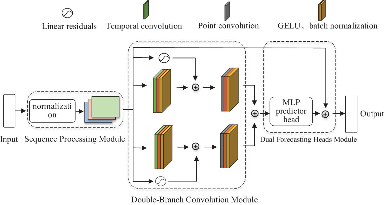
Figure 1: The double-branch convolution model, composed of the sequence processing module (SPM), double-branch convolution module (DBCM), and dual forecasting heads module (DFHM), captures both local and global temporal patterns

3.2.1 Sequence Processing Module

For a univariate time series X1∈RL of length L, traditional deep learning methods typically normalize the data and feed it directly into the network for training, producing the corresponding results. Although traditional methods have made some progress in the field of hydrology, hydrological data can vary due to factors such as time and season, which can still impact the predictive performance of the network model. To address this issue, this experiment employs a segmented value processing approach, where the data is divided into segments for network training to learn local features. The Sequence Processing Module is illustrated in Fig. 2.

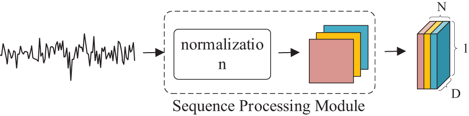
Figure 2: Sequence processing module

Using a segmented value design, the univariate time series X1∈RL is transformed by segmenting it into portions with a segment length of len and a stride of stride. This method extends the input sequence by repeating the stride multiple times. After applying this method, a two-dimensional block is generated to maintain the original relative positions within the sequence. The process can be described by the following formula:

X^2D=Unfold(ReplicationPad(X^1D),size=len,step=stride)(1)

After the Sequence Processing Module processes the data, it becomes possible to adopt methods similar to image processing. The segmented value design decomposes the one-dimensional time series into structured two-dimensional fragments. This two-dimensional format allows for the introduction of spatial considerations, which resemble the nature of image data. As a result, convolution operations can be applied to capture both local and global relationships within the time series [23].

3.2.2 Double-Branch Convolution Module

In time-series forecasting, traditional convolutional networks often model the global relationships within time-series data across multiple scales or branches. However, this approach has drawbacks such as high computational cost, large memory requirements, and increased training difficulty. To better capture temporal relationships in the sequences while reducing model complexity and computation, this paper proposes a double-branch convolutional structure. The design of this structure is inspired by the residual connections in deep learning networks as described in reference [22], allowing outputs to be passed directly without significant modification. The double-branch design enables the construction of a deeper network architecture, which allows the model to capture both global receptive fields and local position features in the input sequence. This capability is especially critical in complex tasks requiring multiple layers of features. The proposed double-branch convolutional structure leverages both temporal convolution and point-wise convolution, enhancing the model’s ability to process temporal dependencies effectively while maintaining computational efficiency.

In the temporal convolution module, assume that after the segmentation processing module, the sequence is divided into N segments, each with a length of len. To expand the receptive field in the temporal convolution, a larger convolution kernel is applied, with the kernel size set based on the len value from the segmentation processing. During this process, the N segments are fed into the network sequentially, and each segment generates a corresponding feature map. These N feature maps are then concatenated in order, forming an output feature map with N channels. Afterwards, the N feature maps are concatenated in sequence, forming an output feature map with N channels. The temporal convolution calculation is given by the following equation:

xlN×D=BN(σ{ConvN(xl−1N×D,stride=K,kernelsize=K)})(2)

where, xlN×D represents the output of the input sequence at layer l, σ is the element-wise nonlinear activation function, specifically the Gaussian error linear units (GELU) function in this case [24].

The temporal convolution module applies the same convolutional kernel to the time-series data, enabling the model to capture underlying periodic patterns. By reusing the same parameters across different sections of the time series, the convolutional kernel extracts features within local regions while also leveraging those features throughout the entire sequence. This mechanism allows for efficient modeling of temporal dependencies. The advantage of temporal convolution lies in its ability to not only identify important features within the time series but also ensure parameter reusability, which enhances data utilization efficiency. This approach enables the model to efficiently learn from the time-series data, maintaining a balance between local feature extraction and global pattern recognition.

When using the temporal convolution module to capture the internal features of each segment, pointwise convolution is applied after the temporal convolution to capture the feature correlations between segments. Temporal convolution deeply learns the complex patterns within each segment, while pointwise convolution captures and integrates the interactions and dynamic relationships between these segments. By introducing pointwise convolution, the model efficiently models the temporal dependencies across different parts of the time series, enhancing the overall representational power of the model. The pointwise convolution is computed as follows:

xl+1A×D=BN(σ{ConvN→A(xlN×D,stride=1,kernelsize=1)})(3)

where, A represents the input to the pointwise convolution.

This model employs separable convolution, achieving superior performance in sequence prediction tasks on the dataset used in this study, surpassing models with attention mechanisms. Moreover, it demonstrates excellent performance when compared to traditional convolutional methods. By carefully tuning the output channel count A of the pointwise convolution layer, the model can control the integration of information between different segments of the sequence, enabling fine-grained optimization of the interactions among time-series features.

This flexibility allows the model to adjust the degree of feature interaction between segments, enhancing the overall predictive accuracy while maintaining computational efficiency. The separable convolution’s ability to isolate spatial and temporal feature extraction makes it a powerful approach for improving time-series prediction tasks, particularly when handling complex dependencies within the data.

3.2.3 Dual Forecasting Heads Module

Traditional LSTM methods typically decompose input sequences, such as by breaking them down based on seasonal variations, before feeding them into the network to generate predictions. Similarly, in the multi-head attention mechanism of the Transformer model, decomposition and aggregation are also utilized to enhance predictive accuracy. Drawing inspiration from the predictive heads used in both models, this paper introduces a dual forecasting head module that incorporates both decomposition and aggregation. The module includes two distinct heads: a nonlinear forecasting head and a linear forecasting head.

When utilizing the forecasting head module for skip connections, the model employs a linear residual forecasting head to extract the overall trend of temporal changes. After the convolutional layers, the model applies both a Multi-Layer Perceptron (MLP) forecasting head and a nonlinear function forecasting head to fit the variations within the sequence. The final prediction is produced by summing the outputs of these heads. Compared to traditional models that use a single linear forecasting head, the dual forecasting head approach enables the model to capture deeper details of sequence changes. This results in a more refined sequence mapping, leading to improved prediction accuracy. The structure of the forecasting heads is illustrated in Fig. 3.

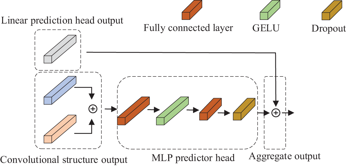
Figure 3: Prediction head structure diagram

4  Experiments

4.1 Datasets and Preprocessing

This dataset consists of daily water and sediment measurement data from over 20 years of operation of the Xiaolangdi Reservoir in China, including inflow/outflow and sediment concentration, offering a comprehensive view of reservoir capacity dynamics. This data captures detailed daily fluctuations in water and sediment quantities, reflecting the reservoir’s capacity variability. By predicting the changes in sediment outflow from the reservoir, the model can reveal future trends in the reservoir’s capacity evolution to a certain extent.

The model’s input dataset integrates seven key indicators to achieve precise predictions of sediment outflow from the reservoir. Specifically, the inputs include: Date (D), Water Level (H), Inflow Volume (If), Inflow Sediment Concentration (Is), Outflow Volume (Of), Outflow Sediment Concentration (Os) and Inflow Water Volume (Iw). These indicators collectively form a multidimensional feature space, providing ample information for the long-term sequence model to learn from. The Sediment Outflow (S) is the sole output variable. The comprehensive prediction model established is:

S=f(D,H,If,IS,Of,OS,Iw)(4)

To overcome the dimensional differences among various features and improve model accuracy, each feature is normalized before being input into the model. This preprocessing step not only accelerates model training and convergence but also maintains the original information of the data. Specifically, normalization is performed using the maximum and minimum values of each feature to standardize the corresponding data, ensuring that the normalized data falls within a uniform scale. This step helps the model learn features more stably during training and reduces the risk of certain features disproportionately influencing the model due to inconsistent dimensions. The normalization formula is as follows:

x′=x−min(xtrain)max(xtrain)−min(xtrain)(5)

where, x is the original feature value, xtrain is the training data, x′ is the data after normalization.

4.2 Experimental Detail

In this experiment, the algorithm used was PaddlePaddle GPU 2.5.1 framework, programming language version: Python 3.7.16, running environment: Linux Ubuntu 20.04 operating system, CPU model: Intel (R) Core (TM) i7-10700 K, CPU clock speed: 3.8 GHz, server memory: 64 GB DDR4, graphics card model: Nvidia RTX A5000, video memory: 24 GB.

4.3 Model Evaluation Indexes and Experimental Results

During the model training process, Mean Square Error (MSE) and Mean Absolute Error (MAE) are used as loss functions for evaluation. In the model testing phase, relative standard error (RSE) and coefficient of determination R2 are introduced as evaluation indicators for the model. This method is used in statistics to measure the accuracy of sample estimation. Due to the use of relative values, it is very useful when comparing sample estimates of different sizes or different variables. The formula of mean square error function loss, mean absolute error loss and relative standard error function is as follows:

mse=1m∑i=1m(yi−f(xi))2(6)

mae=1m∑i=1m|yi−f(xi)|(7)

rse=∑(yi−f(xi))2(yi−x¯)2(8)

where, yi is the measured value for sample i, f(xi) is what the model predicts for the i sample, x¯ is the average value of the measured value.

4.4 Experimental Result

In the model training phase, set the network learning rate to 0.00001, input network batch size to 256, use AdamW [25] optimizer, and have a maximum iteration count of 800. In order to verify the validity of the two-branch convolution model proposed in this paper, the model was compared with the performance of the three benchmark models ITransformer [26], PatchMixer [27] and TSMixer [28] in the reservoir measured data sets. In this experiment, a model comparison experiment was conducted using the actual observational data set of a reservoir to evaluate and compare the performance of several advanced algorithms in the field of time series prediction. The experimental determination coefficients are shown in Table 1, and the comparison of other performance indicators is shown in Fig. 4. The improved DCON model has lower losses and higher determination coefficients, indicating that the DCON model performs better and is more accurate in predicting outbound sediment volume. The DCON’s superior performance can be attributed to its ability to capture both long-term seasonal trends and short-term fluctuations more effectively than the other models. The sequence segmentation and convolutional layers allow the model to identify recurring seasonal patterns in sediment discharge, improving long-term prediction accuracy.

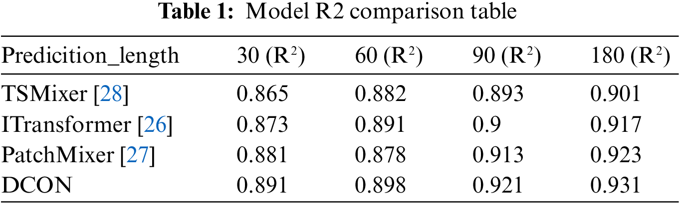
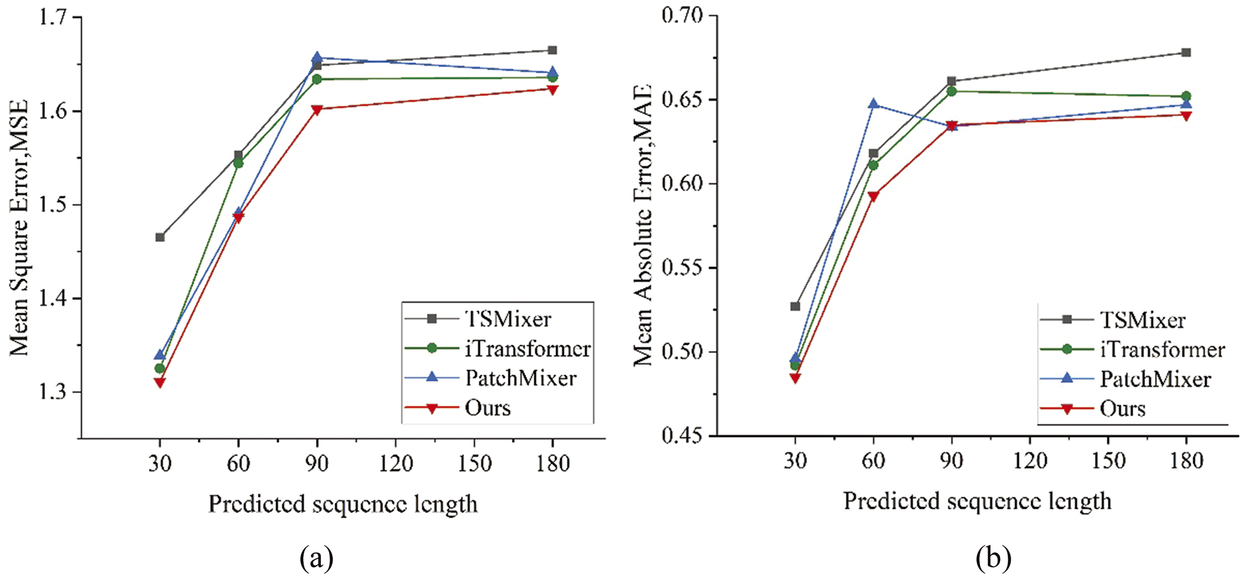
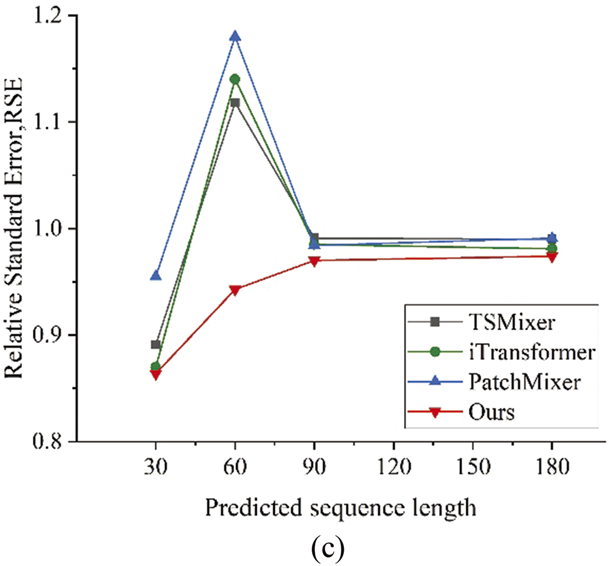
Figure 4: Comparison of training results for multiple sequence lengths, (a) comparison of MSE values of each model; (b) comparison of MAE values of each model; (c) comparison of RSE values of each model

In predictions over a shorter period of time, the improvement effect of DCON is not significant, but the difference compared to other benchmark models is very small. Specifically, the main reason is that the reservoir may experience sudden floods and other events. Non-periodic events such as sudden floods disrupt the model’s ability to predict based on seasonal trends, leading to higher error rates for short-term predictions. Taking into account longer changes, the DCON model performs better overall, indicating that DCON can more accurately describe the correlation between high-dimensional and multivariate variables, and has better adaptability to multiple sequence periods. Its performance in long-term series prediction problems is more accurate and reliable in multiple scenarios. The comparison of losses of four models on multiple prediction sequence lengths is shown in Fig. 4.

Fig. 4 lists the performance metrics of four models in multiple prediction sequence lengths. From the table, it can be seen that the model proposed in this paper exhibits significant advantages compared to other models in water and sediment prediction tasks. In order to observe the differences in prediction among the four models more intuitively, the prediction results of each model at various sequence lengths are divided into Figs. 5–8.

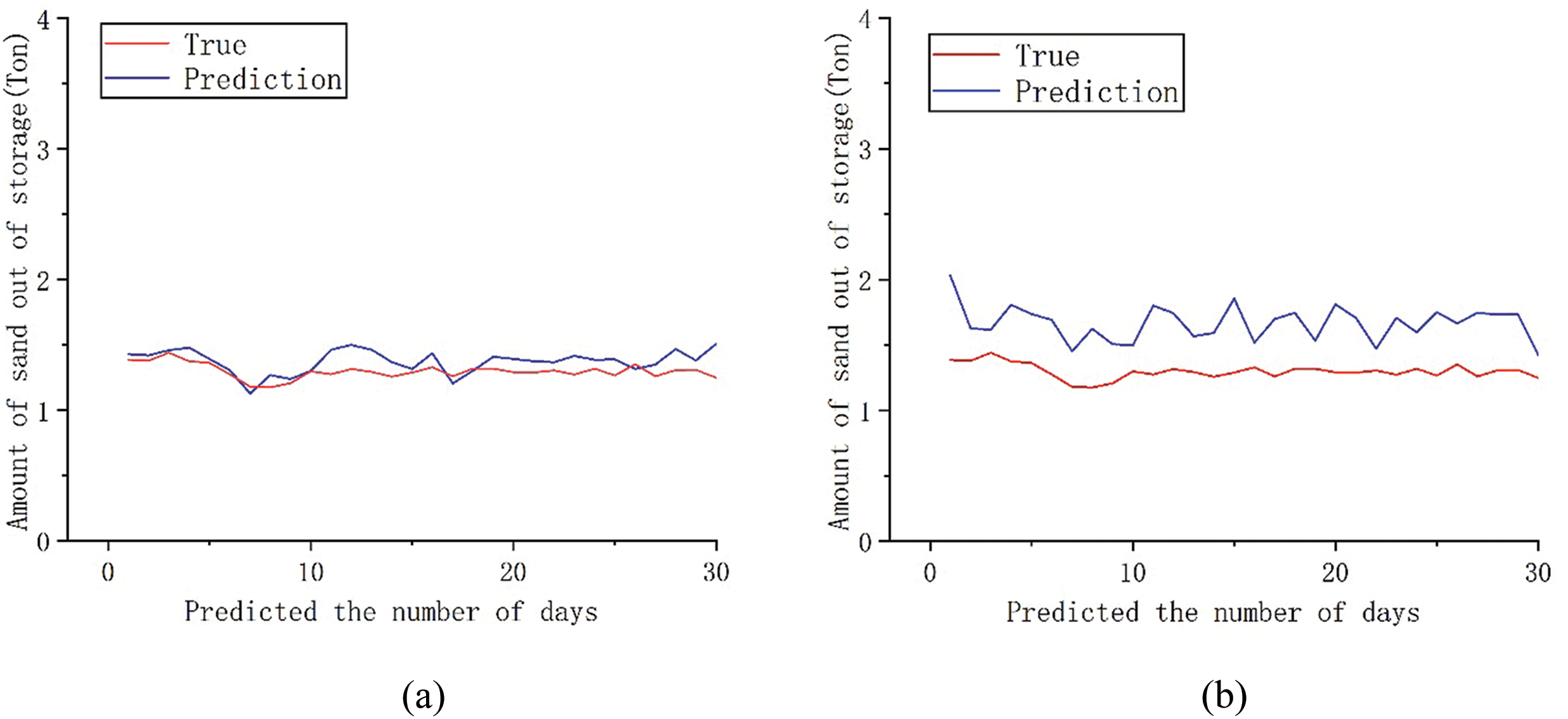
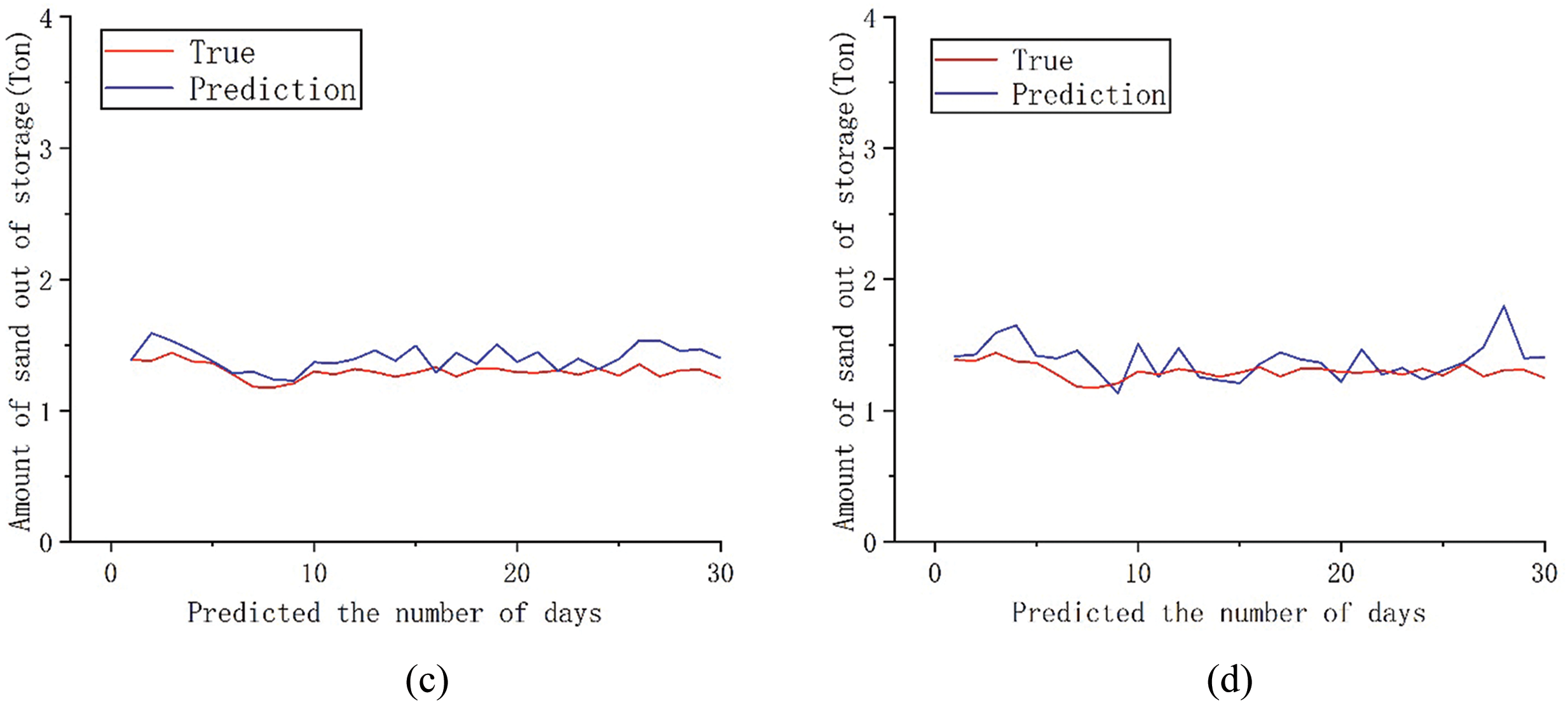
Figure 5: Comparison between the predicted 30-day sediment discharge and the actual value of each model; (a) DCON; (b) ITransformer; (c) PatchMixer; (d) TSMixer

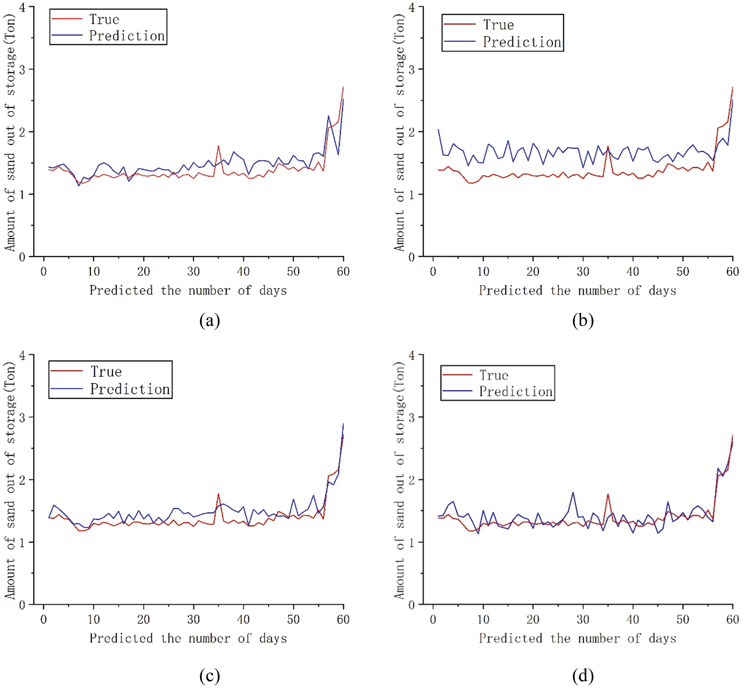
Figure 6: Comparison between the predicted 60-day sediment discharge and the actual value of each model; (a) DCON; (b) ITransformer; (c) PatchMixer; (d) TSMixer

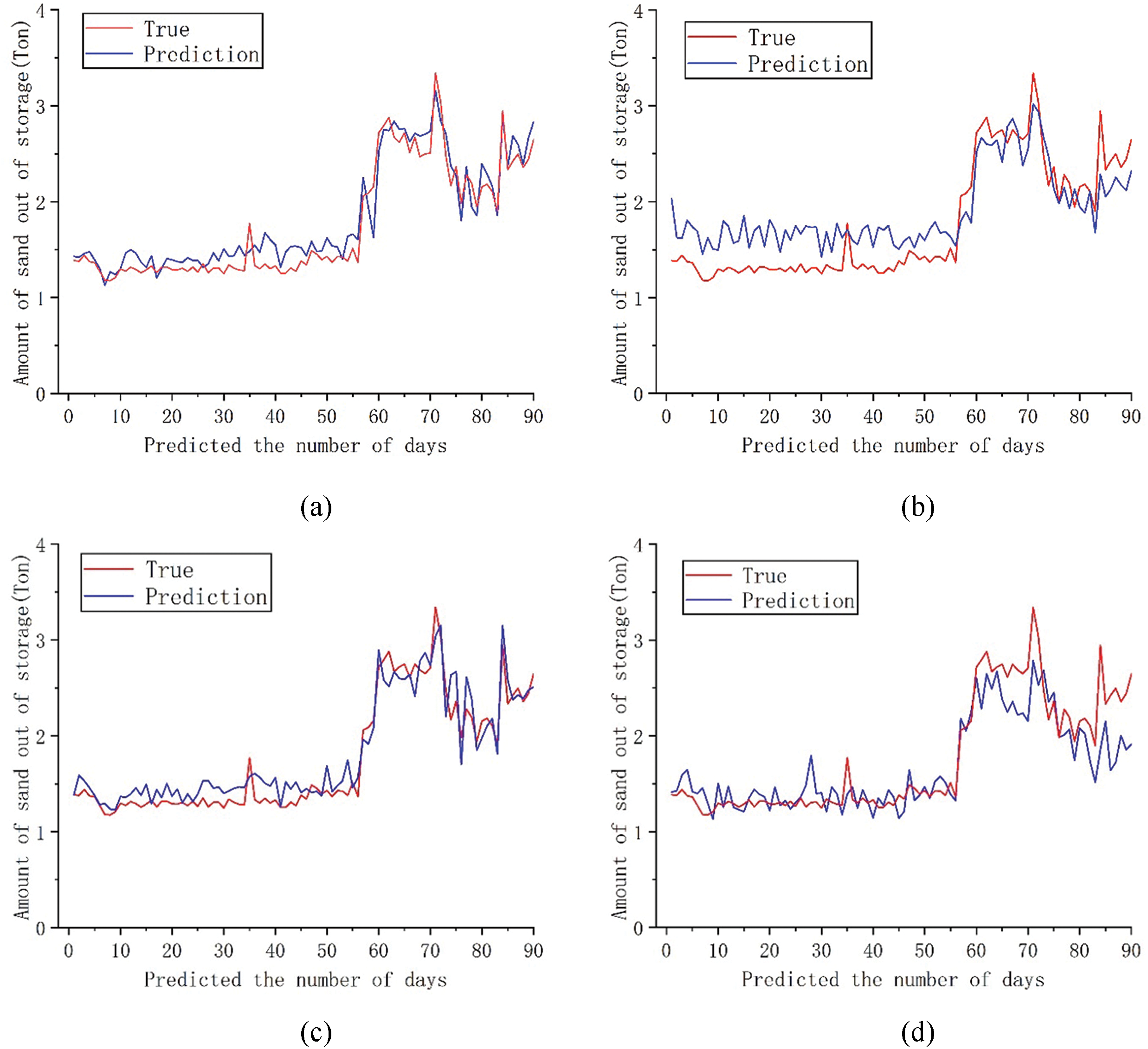
Figure 7: Comparison between the predicted 90-day sediment discharge and the actual value of each model; (a) DCON; (b) ITransformer; (c) PatchMixer; (d) TSMixer

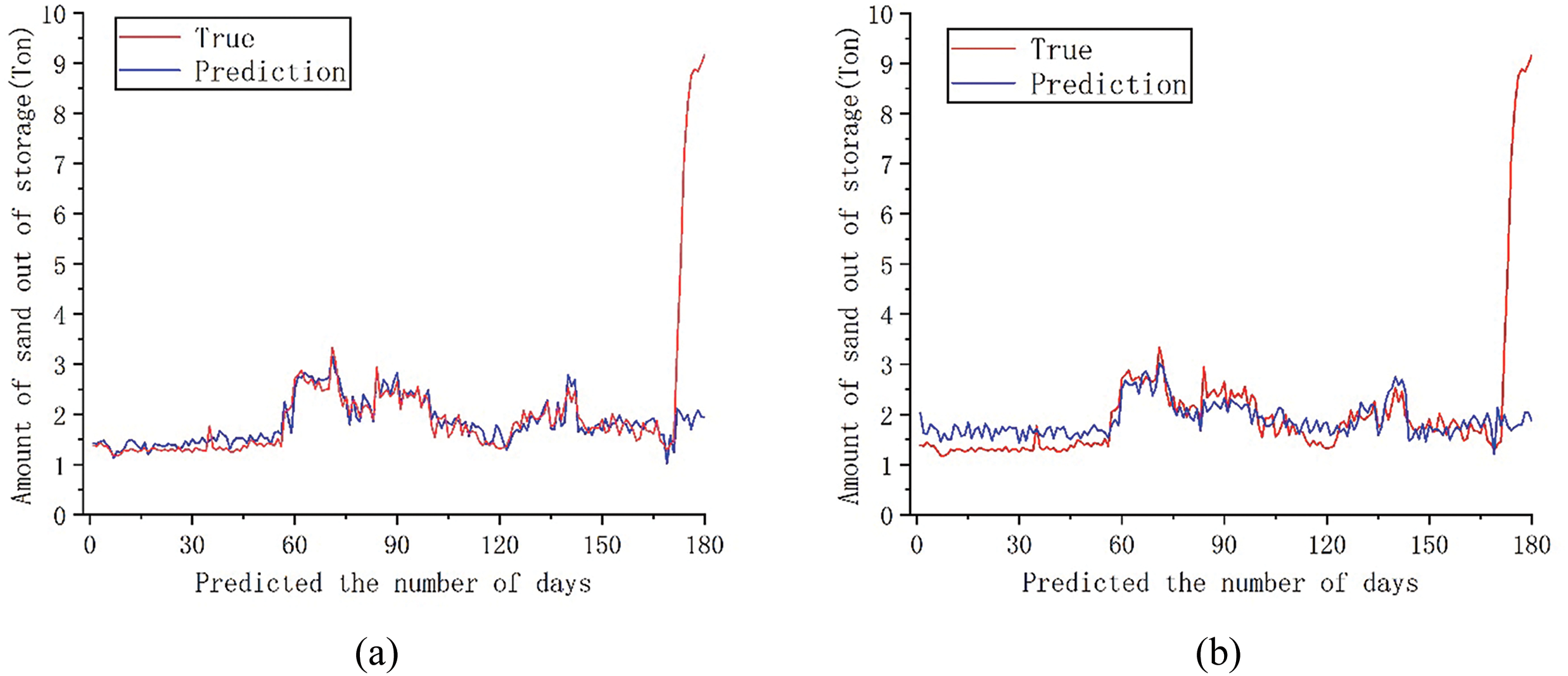
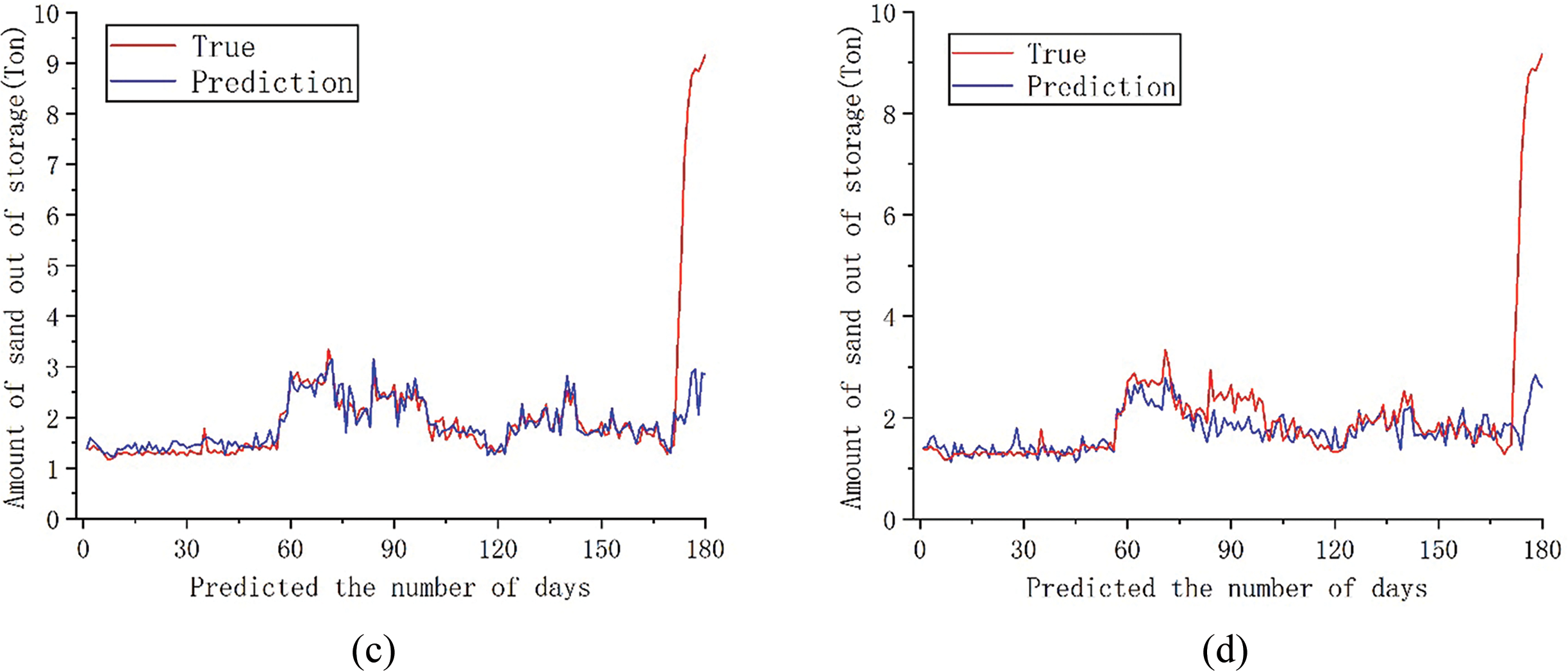
Figure 8: Comparison between the predicted 180-day sediment discharge and the actual value of each model; (a) DCON; (b) ITransformer; (c) PatchMixer; (d) TSMixer

The chart shows that the predicted results of the four models are generally consistent with the true value distribution trend at various sequence lengths. Combined with Table 1, the DCON model outperforms ITransformer, PatchMixer, and TSMixer, with a lower MSE and higher R2, indicating more accurate sediment discharge predictions. By comparing the consistency between predicted values and true values, it can be observed that the dual branch convolution model proposed in this paper can provide predictions that are close to the true values in most cases. Comprehensive analysis shows that after sequence segmentation, feature extraction and residual linking through the dual prediction head and dual branch convolution module can better preserve the sequence feature information, which can enable the model to better focus on the seasonal changes in sediment volume and produce a better model. Comparing the trend of curve changes at the same position as the predicted values and true values of the four models, it can be found that the DCON model used in this article can provide predictions close to the true values in most cases. Compared to other models, the ITransformer model can better predict changes in sediment caused by sudden floods, but its prediction error is relatively large when dealing with slow changes in sediment discharge. From a comprehensive performance perspective, the model used in this article can provide better prediction results and serve as a reference for formulating reservoir output solutions. The analysis results showed that through sequence segmentation and multiple attention of dual prediction heads, combined with the extraction of the characteristics of changes in outbound sediment volume by convolutional layers, the model can better capture long-term seasonal trends and short-term fluctuations, thereby identifying the seasonal sediment discharge patterns that repeatedly appear in outbound sediment volume, and producing better prediction results.

However, the model used in this article and the three benchmark models have not been able to solve the problem of sudden changes in sediment discharge caused by sudden floods in reservoirs. Considering that the reservoir involves a wide water area and a large inflow range, it is affected by non-periodic events such as upstream floods and waterlogging. Sudden floods have disrupted the model’s ability to make periodic predictions based on seasonal trends, resulting in significant errors in predicting short-term sudden changes in sediment levels.

4.5 Ablation Study

To verify the effectiveness of the algorithm improvements used in this study for long-term time-series prediction, ablation experiments were conducted. These experiments assessed the contributions of the sequence processing module, the dual-branch convolution module, and the dual-forecasting heads module on the reservoir’s real-world dataset. The results of the ablation experiments are shown in Table 2.

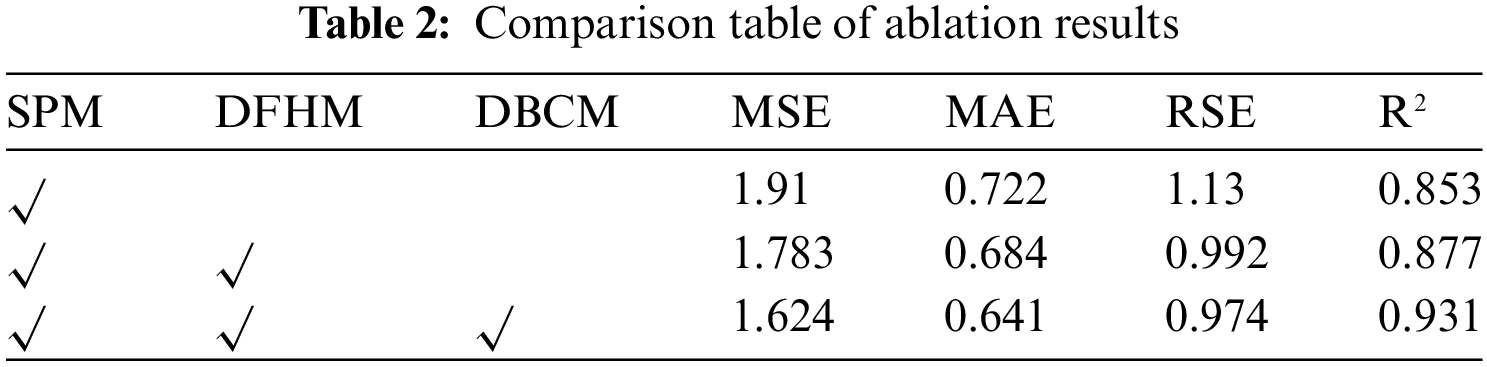
From the ablation experiment results in Table 2, it can be seen that when only the sequence processing module is added to the algorithm, the loss of the model will be slightly reduced, and R2 will also increase accordingly. The experiment found that adding only the sequence processing module greatly improves the training speed of the model, which is closely related to the number of model parameters. Further adding a dual prediction head module to the model increases the number of model parameters. As the number of parameters increases, the model loss further decreases and the model’s coefficient of determination correspondingly improves. The addition of the double-branch convolution module significantly improves MSE and R2 values, demonstrating its importance in extracting temporal features across multivariate time-series. Compared with adding only the sequence processing module, adding the dual branch convolution module reduced MSE, MAE, and RSE by 0.286, 0.081, and 0.078, respectively. The ablation study shows that the full model, with all modules active, provides the best performance, especially in MSE, MAE, RSE and R2, validating the need for each component.

5  Discussion

In terms of current reservoir scheduling policies, deep learning models have brought significant changes and progress. With the development of artificial intelligence technology, it has also caused significant changes in water conservancy. Deep learning simulates the working mode of human brain neural networks, which can process and analyze large amounts of complex data. The development of this technology not only improves the intelligence level of water resource management, but also provides new solutions for the formulation of reservoir scheduling policies.

In formulating traditional reservoir scheduling policies, decision-making often relies more on experience and historical data. Although this method has played an important role in the past, its limitations based on historical experience are gradually becoming apparent in the face of climate change, extreme weather events, and increasing upstream and downstream water demand. However, due to limitations in the way reservoir data is obtained, this article was unable to predict the sediment discharge from other reservoirs and can only simulate and predict based on the data from that reservoir.

Deep learning can also be used to evaluate the effectiveness of different reservoir scheduling schemes. By establishing relevant models and simulating the operation of reservoirs under various scheduling schemes, the advantages and disadvantages of multiple schemes can be intuitively seen. This helps reservoir operation decision-makers choose the optimal solution among numerous options, improving the efficiency and effectiveness of reservoir operation. At the same time as formulating plans, the computational efficiency of deep learning has been significantly improved compared to traditional reservoir scheduling formulas. In the same solution time, deep learning can provide more reference and evaluation solutions for plan makers.

In summary, the development of deep learning technology has brought new opportunities and challenges to the formulation of reservoir scheduling plans. In the formulation of reservoir scheduling policies, the application of deep learning can not only improve the scientific and accurate decision-making, but also promote the sustainable utilization and protection of water resources. In the future, as research continues to deepen and improve, deep learning can play a more important role in this field.

6  Conclusion

In engineering practice, the processed data has non-stationary and nonlinear characteristics. At this time, traditional reservoir scheduling formulas have disadvantages such as poor prediction accuracy and slow calculation. This paper adopts the double branch convolution method, combined with the sequence splitting module, to construct a reservoir outflow sediment prediction model. The prediction model is trained based on daily outflow sediment and flow data, and effectively improves the prediction effect of the model under the premise of the nonlinearity and non-stationarity of the original data. The model in this article is trained in four different scenarios: monthly, bi monthly, quarterly, and semi-annual. The experimental results show that the DCON model used in this article has the best performance. When the outbound sediment volume is the target, the coefficient of determination of the model is 0.931 when predicting for six months. The coefficients of determination of the model for each month, every two months, and every quarter are 0.901, 0.917, and 0.923, respectively. In the experiment, it was found that the dual branch convolution model used in this paper has the following advantages: compared with traditional reservoir scheduling formulas, it can maintain good model prediction accuracy while reducing certain computational practices, proving that the algorithm has good representational power; After the sequence processing and splitting module, the ability to extract features of multiple data lengths has been effectively improved, and the model has shown good predictive performance on various sequence lengths, proving its good robustness. This study currently only uses twenty years of data, and collecting more training data in the future can improve the performance of the DCON model by learning new patterns from new samples. Future research will focus on refining the model to better handle sudden sediment discharge changes caused by reservoir inflow events.

Acknowledgement: I would like to express my heartfelt thanks to my colleagues and friends who participated in the discussion and put forward valuable suggestions.

Funding Statement: National Natural Science Foundation of China (U2243236, 51879115, U2243215), Recipients of funds: Xinjie Li, URL: https://www.nsfc.gov.cn/ (accessed on 25 November 2024).

Author Contributions: The authors confirm contribution to the paper as follows: study conception and design: Hailong Wang, Xinjie Li; data collection: Xinjie Li, Junchao Shi; analysis and interpretation of results: Xinjie Li, Junchao Shi, Hailong Wang; draft manuscript preparation: Junchao Shi. All authors reviewed the results and approved the final version of the manuscript.

Availability of Data and Materials: Data not available due to commercial restrictions.

Ethics Approval: Not applicable.

Conflicts of Interest: The authors declare no conflicts of interest to report regarding the present study.

References

1. J. F. Torres, D. Hadjout, A. Sebaa, F. Martínez-Álvarez, and A. J. Troncoso, “Deep learning for time series forecasting: A survey,” IEEE Big Data, vol. 9, no. 1, pp. 3–21, 2021. doi: 10.1089/big.2020.0159. [Google Scholar] [PubMed] [CrossRef]

2. C. F. Hao, J. Qiu, and F. -F. Li, “Methodology for analyzing and predicting the runoff and sediment into a reservoir,” Water, vol. 9, no. 6, 2017, Art. no. 440. doi: 10.3390/w9060440. [Google Scholar] [CrossRef]

3. P. Chen et al., “Prediction research on sedimentation balance of three gorges reservoir under new conditions of water and sediment,” Sci. Rep., vol. 11, no. 1, 2021, Art. no. 19005. doi: 10.1038/s41598-021-98394-x. [Google Scholar] [PubMed] [CrossRef]

4. M. B. Idrees, M. Jehanzaib, D. Kim, T. -W. Kim, “Comprehensive evaluation of machine learning models for suspended sediment load inflow prediction in a reservoir,” Stoch. Environ. Res. Risk Assess., vol. 35, no. 9, pp. 1805–1823, 2021. doi: 10.1007/s00477-021-01982-6. [Google Scholar] [CrossRef]

5. H. Nagy, K. Watanabe, and M. Hirano, “Prediction of sediment load concentration in rivers using artificial neural network model,” J. Hydraul. Eng., vol. 128, no. 6, pp. 588–595, 2002. doi: 10.1061/(ASCE)0733-9429(2002)128:6(588). [Google Scholar] [CrossRef]

6. N. AlDahoul et al., “Suspended sediment load prediction using long short-term memory neural network,” Sci. Rep., vol. 11, no. 1, 2021, Art. no. 7826. doi: 10.1038/s41598-021-87415-4. [Google Scholar] [PubMed] [CrossRef]

7. H. Iraji, M. Mohammadi, B. Shakouri, and S. G. Meshram, “Predicting reservoir volume reduction using artificial neural network,” Arab J. Geosci, vol. 13, no. 17, 2020, Art. no. 835. doi: 10.1007/s12517-020-05772-2. [Google Scholar] [CrossRef]

8. H. Wu, J. Xu, J. Wang, and M. J. Ainips Long, “Autoformer: Decomposition transformers with auto-correlation for long-term series forecasting,” in Proc. 35th Int. Conf. Neural Inform. Process. Syst. (NeurIPS 2021), 2021, vol. 34, pp. 22419–22430. doi: 10.48550/arXiv.2106/13008. [Google Scholar] [CrossRef]

9. S. Ogunjo, A. Olusola, and C. Olusegun, “Predicting river discharge in the niger river basin: A deep learning approach,” Appl. Sci., vol. 14, no. 1, 2023, Art. no. 12. doi: 10.3390/app14010012. [Google Scholar] [CrossRef]

10. A. Zeng, M. Chen, L. Zhang, and Q. Xu, “Are transformers effective for time series forecasting?” Proc. AAAI Conf. Artif. Intell., vol. 37, no. 9, pp. 11121–11128, 2023. doi: 10.1609/aaai.v37i9.26317. [Google Scholar] [CrossRef]

11. H. A. Afan, A. El-Shafie, Z. M. Yaseen, M. M. Hameed, W. H. M. Wan Mohtar and A. J. Hussain, “ANN based sediment prediction model utilizing different input scenarios,” Water Resour. Manage., vol. 29, no. 4, pp. 1231–1245, 2015. doi: 10.1007/s11269-014-0870-1. [Google Scholar] [CrossRef]

12. S. Ma, J. G. Cao, and R. S. Letters, “A two-branch neural network for gas-bearing prediction using latent space adaptation for data augmentation—An application for deep carbonate reservoirs,” IEEE Geosci. Remote Sens. Lett., 2024. doi: 10.1109/LGRS.2024.3436836. [Google Scholar] [CrossRef]

13. M. Xu, M. Liu, Y. Liu, S. Liu, and H. Sheng, “Dual-branch feature interaction network for coastal wetland classification using sentinel-1 and 2,” IEEE J. Sel. Top. Appl. Earth Obs. Remote Sens., vol. 17, pp. 14368–14379, 2024. doi: 10.1109/JSTARS.2024.3440640. [Google Scholar] [CrossRef]

14. S. Bai, J. Z. Kolter, and V. J. Koltun, “An empirical evaluation of generic convolutional and recurrent networks for sequence modeling,” 2018. arXiv:1803.01271. [Google Scholar]

15. M. Liu et al., “Scinet: Time series modeling and forecasting with sample convolution and interaction,” in 36th Conf. Neural Inform. Process. Syst. (NeurIPS 2022), 2022, vol. 35, pp. 5816–5828. [Google Scholar]

16. H. Wang, J. Peng, F. Huang, J. Wang, J. Chen, and Y. Xiao, “MICN: Multi-scale local and global context modeling for long-term series forecasting,” in Eleventh Int. Conf. Learn. Represent., 2023. [Google Scholar]

17. H. Wu, T. Hu, Y. Liu, H. Zhou, J. Wang, and M. J. Long, “TimesNet: Temporal 2D-variation modeling for general time series analysis,” 2022, arXiv:2210.02186. [Google Scholar]

18. C. Szegedy et al., “Going deeper with convolutions,” in Proc. IEEE Conf. Comput. Vis. Pattern Recognit., 2015, pp. 1–9. [Google Scholar]

19. S. J. Ioffe, “Batch normalization: Accelerating deep network training by reducing internal covariate shift,” 2015, arXiv:1502.03167. [Google Scholar]

20. A. G. J. Howard, “MobileNets: Efficient convolutional neural networks for mobile vision applications,” 2017, arXiv:1704.04861. [Google Scholar]

21. F. Chollet, “Xception: Deep learning with depthwise separable convolutions,” in Proc. IEEE Conf. Comput. Vis. Pattern Recognit., 2017, pp. 1251–1258. [Google Scholar]

22. K. He, X. Zhang, S. Ren, and J. Sun, “Deep residual learning for image recognition,” in Proc. IEEE Conf. Comput. Vis. Pattern Recognit., 2016, pp. 770–778. [Google Scholar]

23. L. Liu, J. Chen, P. Fieguth, G. Zhao, R. Chellappa and M. J. Pietikäinen, “From BoW to CNN: Two decades of texture representation for texture classification,” Int. J. Comput. Vis., vol. 127, no. 1, pp. 74–109, 2019. doi: 10.1007/s11263-018-1125-z. [Google Scholar] [CrossRef]

24. Y. Guo, D. Zhou, W. Li, and J. A. Cao, “Deep multi-scale Gaussian residual networks for contextual-aware translation initiation site recognition,” Expert Syst. Appl., vol. 207, no. 10, 2022, Art. no. 118004. doi: 10.1016/j.eswa.2022.118004. [Google Scholar] [CrossRef]

25. I. J. Loshchilov, “Decoupled weight decay regularization,” 2017, arXiv:1711.05101. [Google Scholar]

26. Y. Liu et al., “iTransformer: Inverted transformers are effective for time series forecasting,” 2023, arXiv:2310.06625. [Google Scholar]

27. Z. Gong, Y. Tang, and J. J. Liang, “PatchMixer: A patch-mixing architecture for long-term time series forecasting,” 2023, arXiv:2310.00655. [Google Scholar]

28. S. A. Chen, C. L. Li, N. Yoder, S. O. Arik, and T. J. Pfister, “TSMixer: An All-MLP architecture for time series forecasting,” 2023, arXiv:2303.06053. [Google Scholar]