A Software Defect Prediction Method Using a Multivariate Heterogeneous Hybrid Deep Learning Algorithm

1  Introduction

In the field of software engineering, improving software quality and reliability is always an important and continuous challenge. Effective identification of software defects plays a key role in reducing operation and maintenance costs, improving user satisfaction and ensuring software security. In this context, Software Defect Prediction (SDP) technology has emerged. With SDP, development teams are able to identify potential defects in the early stages of the software lifecycle, thus avoiding costly fixes at a later stage. Studies have shown that the cost of remediation increases exponentially with the time of defect discovery [1]. In addition, SDP can help development and testing teams achieve more targeted testing by focusing on modules with higher defect risk rather than distributing resources evenly across all codes. This prioritization strategy effectively improves testing efficiency and reduces unnecessary testing overhead. At the same time, SDP can help the maintenance team locate and fix problems more quickly during operation and maintenance, shortening fault recovery time. The data-driven testing and maintenance strategy not only improves the overall operation and maintenance efficiency, but also enhances team collaboration and the effectiveness of problem solving.

1.1 Motivation

Software Defect Prediction (SDP) utilizes historical project datasets, after data cleaning and feature selection, to train prediction models to identify defect-containing files, classes, or statements in new projects to improve software quality and security. The existing studies can be divided into three directions:

(1)   Apply artificial intelligence techniques to manually designed software metric data for defect prediction, e.g., Chidamber and Kemerer (CK) metrics [2], MCcabe metrics [3], Halstead metrics [4].

(2)   Extract defective features using program tree representations and deep learning techniques.

(3)   Mix manually designed metric data and program syntsax trees as defect prediction factors to predict software defects by deep learning techniques.

Artificially designed software metrics data can correctly reflect the statistical characteristics of the software code and measure the complexity of the code from different perspectives, Chen et al. [5] proposed software defect prediction based on nested superposition of integrated learning models and heterogeneous feature selection; Zain et al. [6] proposed a novel one-dimensional convolutional neural network deep learning model and applied this model to software defect prediction; Khleel et al. [7] predicted software defects based on Convolutional Neural Networks (CNN) and Gated Recursive Units (GRU) combined with synthetic few oversampling techniques. The studies in the above literature proved that software metrics data and software defects are correlated, but software metrics data cannot reflect the specific structural information of the code and internal control information. For example, as shown in Fig. 1, the code above has no defects while the code below has defects under the same metrics such as the number of lines of code and complexity. Therefore, it is difficult to comprehensively measure the characteristic information of the code through a single software metric data.

Figure 1: An example for bugs

To overcome the limitations of code metrics data to explain code features, researchers have turned to parse source code and extract syntax trees to enrich semantic and structural information to predict potential defects. This approach provides new perspectives for software defect prediction research. Farid et al. [8] use a hybrid model (CBIL) of convolutional neural network (CNN) and bidirectional long short-term memory (Bi-LSTM) based on AST syntax tree for software defect prediction; Dam et al. [9] construct a tree-structured long short-term memory network to match the abstract syntax tree of source code for software defect prediction; Fan et al. [10] used recurrent neural network of attention for software defect prediction based on Abstract Syntax Tree (AST). The studies in the above literature proved that AST syntax trees can reflect software defect information, but when using AST to extract defect predictors, the vast majority of defect prediction models treat AST nodes as linear sequences and use natural language models to generate embedding vectors for the sequences, ignoring the structural information of AST syntax trees.

Other researchers perform defect prediction by fusing code metric data and AST. Wang et al. [11] proposed a gated hierarchical long short-term memory network model and applied this model to extract semantic features and predict software defects from code metric data and abstract syntax trees of source code files; Zhang et al. [12] utilized Convolutional Neural Networks (CNNs) and Attention Based Mechanisms based of Long and Short-Term Memory (Bi-LSTM+Attention) respectively to extract valuable features from code metric data, AST syntax tree and other feature data, and integrate all the sub-models through integrated learning method to get the final defect prediction model. The above literature enriches the defect prediction input data feature information, but when fusing different data features, the existing models often do not perform in-depth analysis for different types of data features, but uniformly adopt the same model for prediction. This may lead to poor model prediction accuracy.

In view of the above analysis, we propose a multivariate heterogeneous hybrid deep learning algorithm for software defect prediction(DP-MHHDL). In this method, we first obtain the quality metric data, abstract syntax tree and file dependency network of the code through the analysis of the source code, and then extract the deep features by using the graph convolutional neural network optimization model based on adjacency topology and spatial topology, the Convolutional Neural Network-Bidirectional Long Short-Term Memory (CNN-BiLSTM) hybrid neural network model, and the TabNet model, respectively, and then finally, the extracted deep features are fused to obtain the final defect prediction framework is obtained by fusing the extracted deep features. The proposed framework is applied to cross version software defect prediction within a project. The experimental data comes from 10 projects in the promise defect repository, and the proposed framework is evaluated using three metrics: F1, Area under the curve (AUC), and Matthews correlation coefficient (MCC). The experimental results show that the proposed algorithm multivariate heterogeneous hybrid deep learning algorithm for defect prediction (DP-MHHDL) is the state-of-the-art approach.

1.2 Contributions

The main contributions of this paper are as follows:

(1)   A graph convolutional neural network optimization model based on adjacency topology and spatial topology is proposed to identify defective software modules from AST abstract syntax trees.

(2)   A mixed deep learning frame from Polyisomerization Data is proposed. Three types of heterogeneous data, code syntax, code quality metrics and code dependency networks, are merged.

(3)   In the experiments of this paper, We designed a large number of experiments to prove the effectiveness of the proposed framework through the indicators F1, AUC, and MCC. The experimental results show that the proposed framework is superior to the existing state-of-the-art methods.

1.3 Organization

The remainder of the paper is organized as follows. Section 2 briefly describes the background knowledge related to the software defect prediction framework for multivariate heterogeneous hybrid deep learning models. Section 3 elaborates on the software defect prediction framework for multivariate heterogeneous hybrid deep learning models. Section 4 demonstrates our experimental setup. Section 5 shows the results of our experiments. Section 6 presents related work. Section 7 discusses threats to validity. Section 8 summarizes our work and looks ahead to future research.

2  Background

In order to clearly introduce our approach, it is necessary to briefly introduce the deep learning model and related technologies involved in our approach.

2.1 Convolutional Neural Network

Convolutional Neural Network (CNN) is a deep learning technique that parses data by mimicking the processing of the human brain. CNNs have achieved remarkable success in the field of computer vision due to their excellent image recognition capabilities. CNNs typically consist of a convolutional layer, an activation layer, a pooling layer, and a fully connected layer. The convolutional layer extracts features from the input data through convolutional operations; the activation layer introduces nonlinear factors to increase the expressive power of the network; the pooling layer is used to reduce the spatial size of the features and reduce the computational effort; and the fully connected layer will map the features to the final output space. Due to its excellent feature extraction ability, Li et al. [13] innovatively applied convolutional neural network (CNN) to the field of software defect detection. by extracting the labeled vectors from the abstract syntax tree (AST) of a program and transforming them into numeric vectors through mapping and word embedding, they successfully utilized CNN’s ability to extract spatial hierarchical features to achieve binary classification detection of software defects. although CNN is good at extracting spatial structural features, it is unable to extract sequential features, so some researchers proposed the long and short-term memory neural network [14].

2.2 Long ShortTerm Memory Network

Long Short-Term Memory (LSTM) is a special Recurrent Neural Network (RNN) architecture specialized in dealing with long-term dependency problems in sequential data. Its core mechanism lies in the introduction of a unique gating mechanism, where the gating unit consists of a forgetting gate, an input gate and an output gate. The forgetting gate is responsible for deciding what information to keep from the previous moment’s unit state, the input gate decides which of the current moment’s input information should be integrated into the unit state, and the output gate regulates how much information should be output from the unit state. The structure of the LSTM network is shown in Fig. 2, and similar to the CNN, Deng et al. [15] have used the code abstraction grammar tree as the input to the LSTM model for conducting a study on software defect prediction.

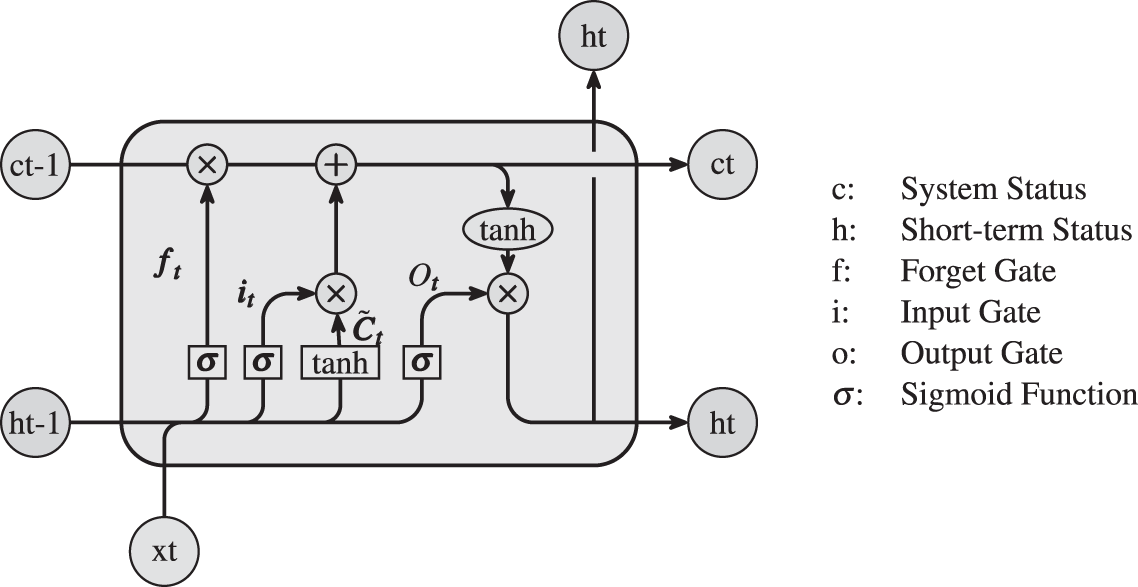
Figure 2: Schematic representation of LSTM model

2.3 Graph Convolutional Neural Networks

Different from the traditional network models of CNN and LSTM that can only be used to process grid-structured data, Graph Convolutional Neural Networks (GCNs) is a more powerful deep learning model, especially suitable for processing data with complex topology. By extending traditional convolutional operations to graph data, GCNs are able to efficiently aggregate information about neighboring nodes, capture spatial dependencies between nodes, and learn embedded representations of nodes. Graph Convolutional Neural Networks (GCNs) can be applied to tasks such as node prediction and graph classification due to their excellent performance. In the node prediction task, GCNs are capable of accurately predicting the attributes or labels of a node by learning the node’s graph structure information and node features. And in the task of graph classification, GCNs can realize level classification of graphs by feature extraction and classification of the whole graph structure. In the field of software defect detection, Šikić et al. [16] proposed a source code software defect prediction model based on graph neural networks, which proved the effectiveness of the graph neural network model.

2.4 TabNet

In the field of structured data mining, traditional machine learning models are still dominant due to the challenges of deep learning models in dealing with sparse and small sample datasets, and the lack of interpretability of the models themselves. In 2019, Google introduced the TabNet model [17], which mimics the behavior of a decision tree using the idea of a sequential attention mechanism that consists of a series of decision steps, each of which selects relevant features and updates the internal representation of the data. This mechanism allows the model to efficiently capture complex nonlinear relationships between features, making it very effective for structured data feature extraction. The TabNet network model has three important properties:

(1)   The model works directly with tabular data without pre-processing, and uses gradient descent-based optimization, making it easy to incorporate into an end-to-end model.

(2)   At every decision time step, the sequential attention model is utilized to select important features and learn the most salient features to make the model interpretable.

(3)   TabNet shows the same modeling effect as other models in both classification and regression. The TabNet model has been successfully applied to business areas such as credit risk prediction and disease prediction, but so far this model has not been applied to the application area of software defect prediction.

3  Approach

Convolutional Neural Networks (CNN), Long Short-Term Memory Networks (LSTM), Graph Convolutional Neural Networks (GCN), and TabNet models each have their own unique advantages in processing data. Specifically, CNN is suitable for processing image data with local spatial structure and some 1D temporal data, and can effectively extract local features, while LSTM is good at processing sequential data with strong temporal order, especially in tasks that need to capture long-term dependencies, and GCN is suitable for processing graph-structured data, which is able to effectively capture the relationships and structural information between nodes in the graph by aggregating information from neighboring nodes, and TabNet is designed for processing graph-structured data, which is able to efficiently extract structural information. TabNet, on the other hand, is designed for tabular data and utilizes the attention mechanism to automatically select important features, thus reducing the reliance on manual feature engineering. Based on the characteristics of the above four models, this chapter proposes a hybrid deep learning model that aims to improve the performance of defect prediction.

In most previous studies, researchers conducted defect prediction using either static metric data or abstract syntax trees as standalone data sources. A few studies have combined both data types for defect prediction, but these efforts often overlooked the distinct characteristics of each data source, applying the same model uniformly. To maximize the extraction of valuable features from each data source, this study proposes a multivariate heterogeneous hybrid deep learning algorithm for software defect prediction. As illustrated in Fig. 3, the DP-MHHDL first extracts three types of data-abstract syntax trees, file dependency relationships, and code quality metrics-from labeled source code files. Next, for the abstract syntax tree data, a graph convolutional neural network optimization model based on adjacency topology and spatial topology is constructed to extract defective feature information, for the file dependency data, a hybrid CNN-Bilstm neural network model is constructed to extract defective feature information, and for the code quality metric data, a TabNet model is used to extract defective feature information, and finally the features extracted from the models are fused and passed through a fully connected neural network to predict whether the software is defective or not. Finally, the features extracted from each model are fused and passed through the fully connected neural network to predict whether the software has defects or not.

Figure 3: Overall architecture

3.1 Data Processing

3.1.1 AST Extraction and Feature Coding

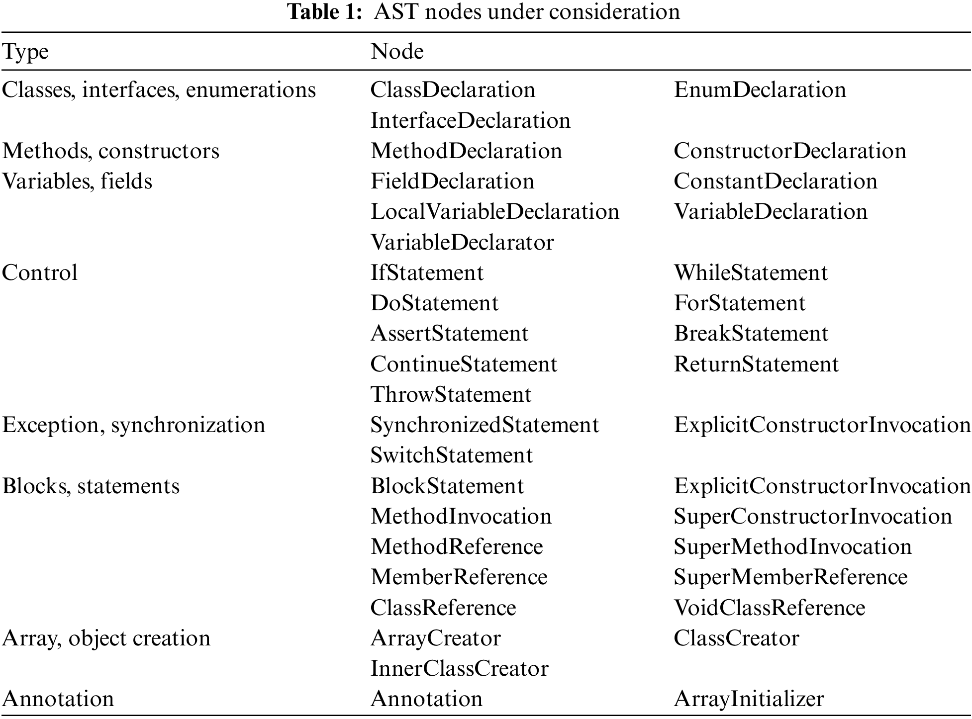
AST expresses the programming language structure in the form of tree visualization, each node represents a structure of the source code, e.g., control node, method declaration node, etc. By parsing the AST tree, code syntax error checking, change code checking and so on can be realized quickly. This study mainly focuses on java code for defect prediction, so we use the open source python library Javalang to extract the AST structure from the source code, and the extracted structure is shown in Fig. 4. The AST node types of Java files contain 78 categories, based on the research of others [12,18], we selected 39 node types related to defect prediction, and the selected node types and node names are shown in Table 1. Considering that the number of different node types in the source code file may have an impact on the quality of the code, e.g., good code should not contain too many nested control statements; more loops in the source code file will have an adverse effect on the readability of the code and defect localization. Therefore, when constructing the connection of the selected 39 node edges, we not only consider the connection relationship of the contextual semantics between the nodes, but also add edges to the node names of the same type.

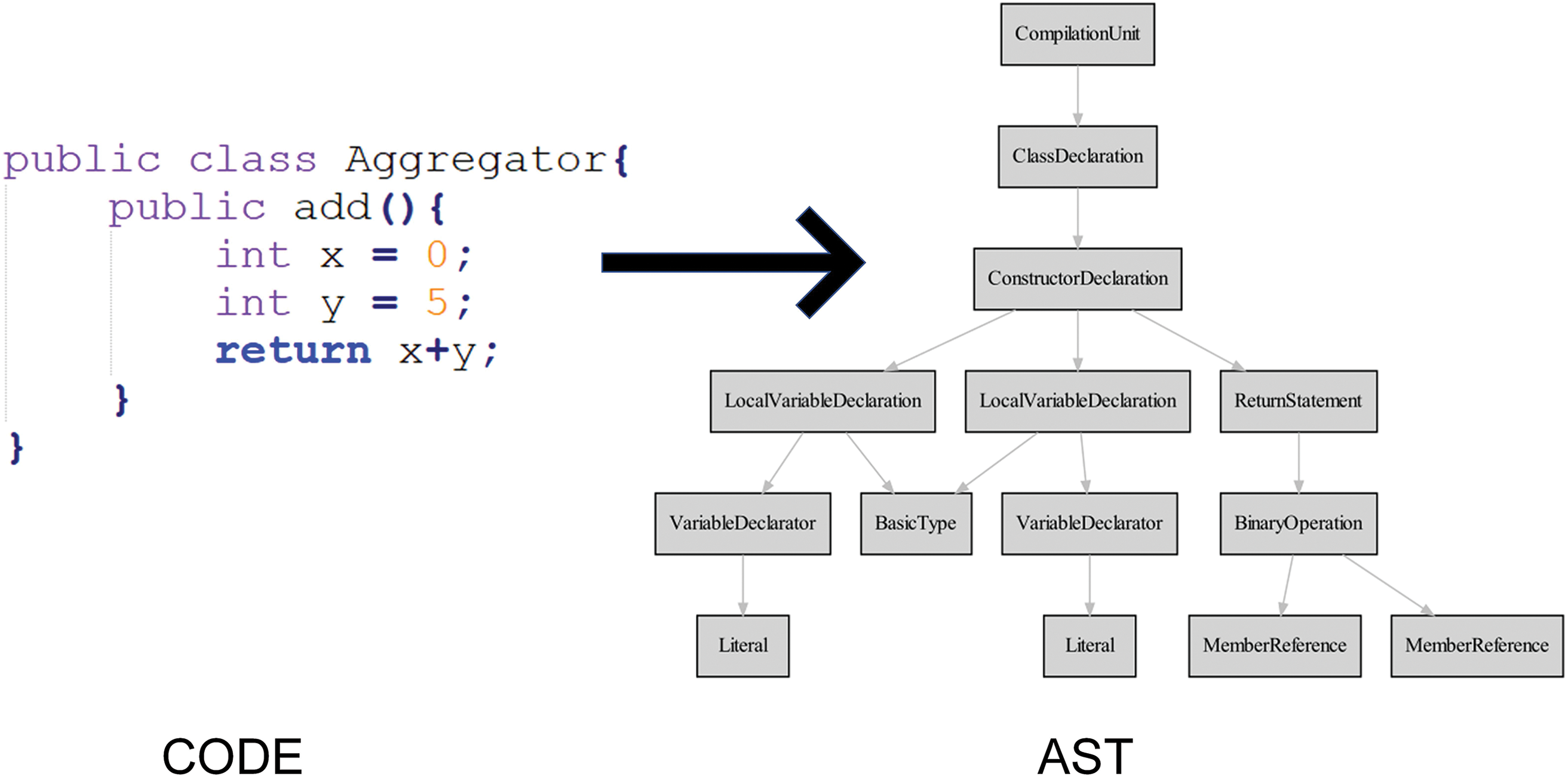
Figure 4: Java code and corresponding abstract syntax tree case

Based on the encoding of the AST graph, we mainly use the unique heat encoding to represent the node features, in addition to that, from the AST we also extracted the contextual semantic based adjacency matrix and the spatial topology matrix based on the same type of nodes respectively.

3.1.2 Code Dependency Network (CDN) Extraction and Feature Coding

AST retains the syntactic semantic information of the source code of individual files, but it cannot reflect the importance of individual files in the whole project engineering. In order to obtain the feature information of a single file in the project engineering, we firstly use the static code analysis tool Understand to generate the class dependency invocation relationship graph for the project engineering, the class dependency invocation relationship is shown in Fig. 5, where each node in the network represents one class, and the edges represent the dependency relationship between two class nodes, and secondly, in order to express the feature information of each node, we generate the class dependency invocation relationship graph for each file (i.e., the class dependency invocation relationship in the graph) by applying the Node2Vec to our class dependency call relationship graph, thus generating rich feature vectors for each file (i.e., node in the graph), the learned vectors contain information such as the relationship between nodes and the network structure. Finally, we can use the obtained vectors for each node to predict whether it is defective or not.

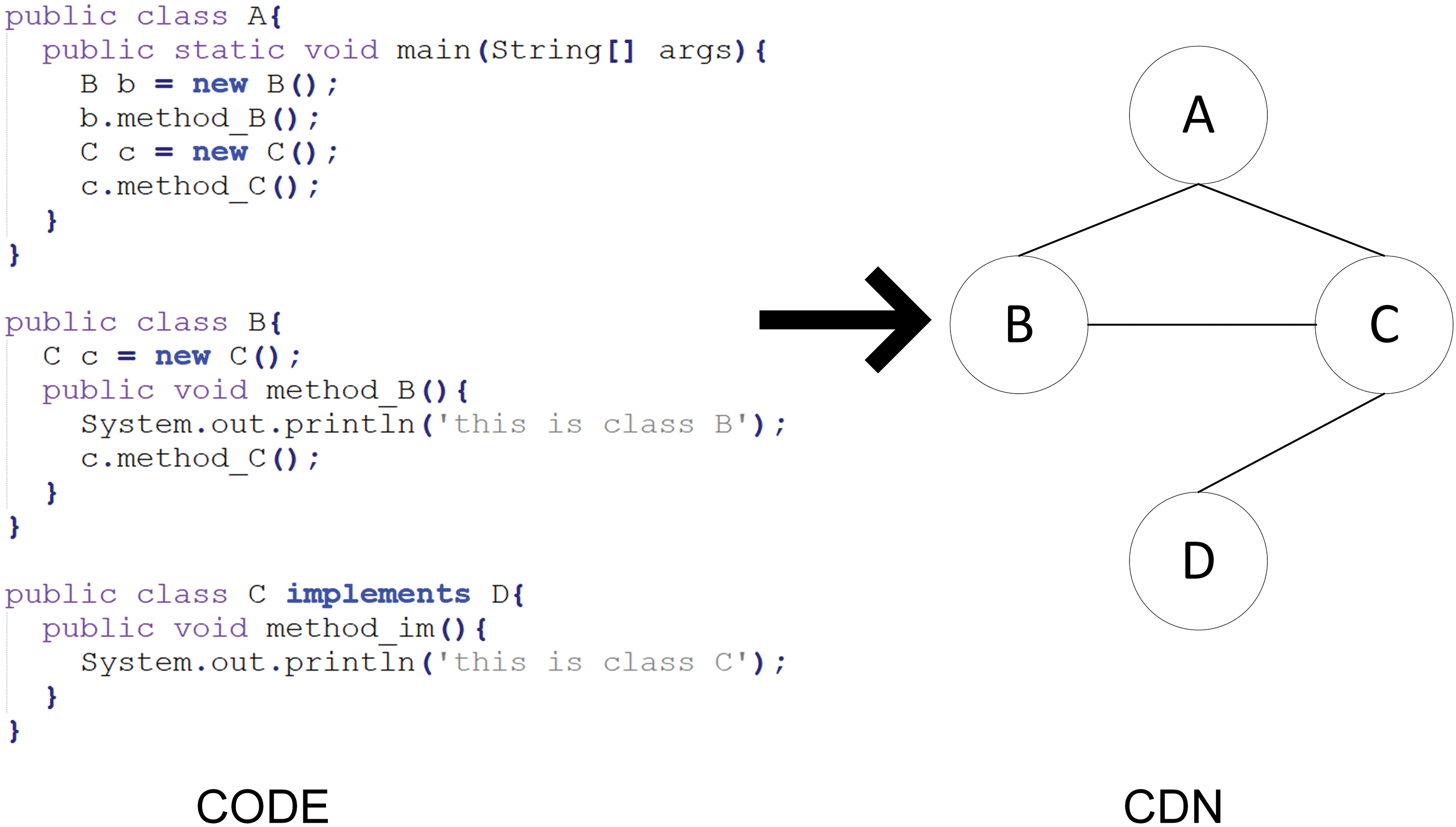
Figure 5: Java code and corresponding Code Dependency Network (CDN)

3.1.3 Code Quality Metrics Data Extraction

Traditional static code quality metrics have been shown to correlate with software defects [11,19–21], Based on previous studies, we selected 20 metrics that correlate with software defects, and the selected metrics are shown in Table 2.

Each software metric has a different scale, so in order to avoid bias towards certain key features, the metric metadata were normalized with the following normalization formula:

xi~=xi−x¯δ(1)

where x¯ is the mean of the specified metric element data, and δ is the standard deviation.

3.2 Design of Model

3.2.1 Models for Handling Graph-Structured Data

We employ a unique deep learning model, a graph convolutional neural network optimization model based on adjacency topology and spatial topology, specifically designed to process abstract syntax trees (ASTs) for codes. The inputs to the model are mainly graph representations of the AST, specifically the node features X, the node adjacency matrix A, and the spatial topology matrix K, which is used to characterize the spatial feature relationships among nodes. In constructing the model, a 3-layer graph convolutional neural network is used, and the overall modle architecture is shown in Fig. 6.

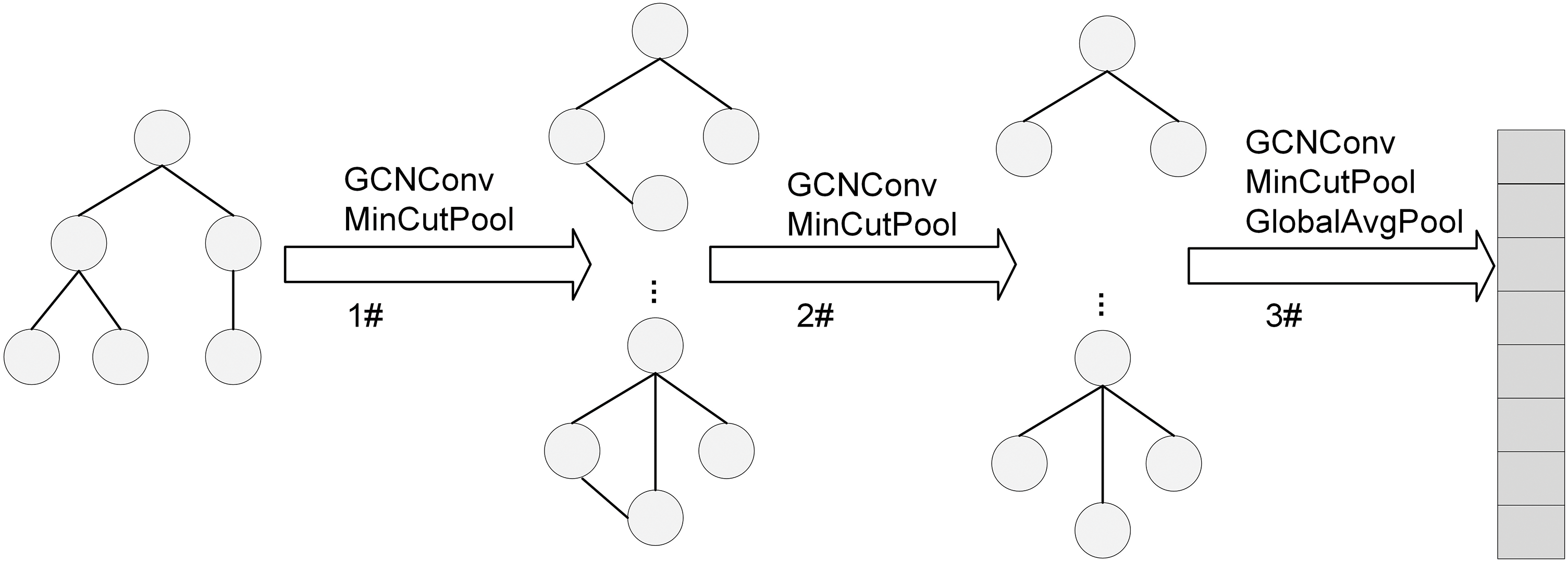
Figure 6: Model architecture

In the first layer of the model, the model structure is shown in Fig. 7, we first deployed two parallel GCN convolutional layers, based on the node features X, the adjacency matrix A and the spatial feature matrix S to perform operations to generate new node features XA and XS, and such a design makes the model able to extract the spatial features from two different dimensions: on the one hand, capturing the direct connections between nodes through the adjacency matrix; on the other hand, through the spatial feature matrix S mining more complex spatial relationships among nodes. The goal of this step is to make full use of the graph structure to capture the neighboring features and spatial features of the nodes, and map these features into a high-dimensional space, so as to provide rich information for subsequent analysis and learning. The specific implementation is shown in the following equation:

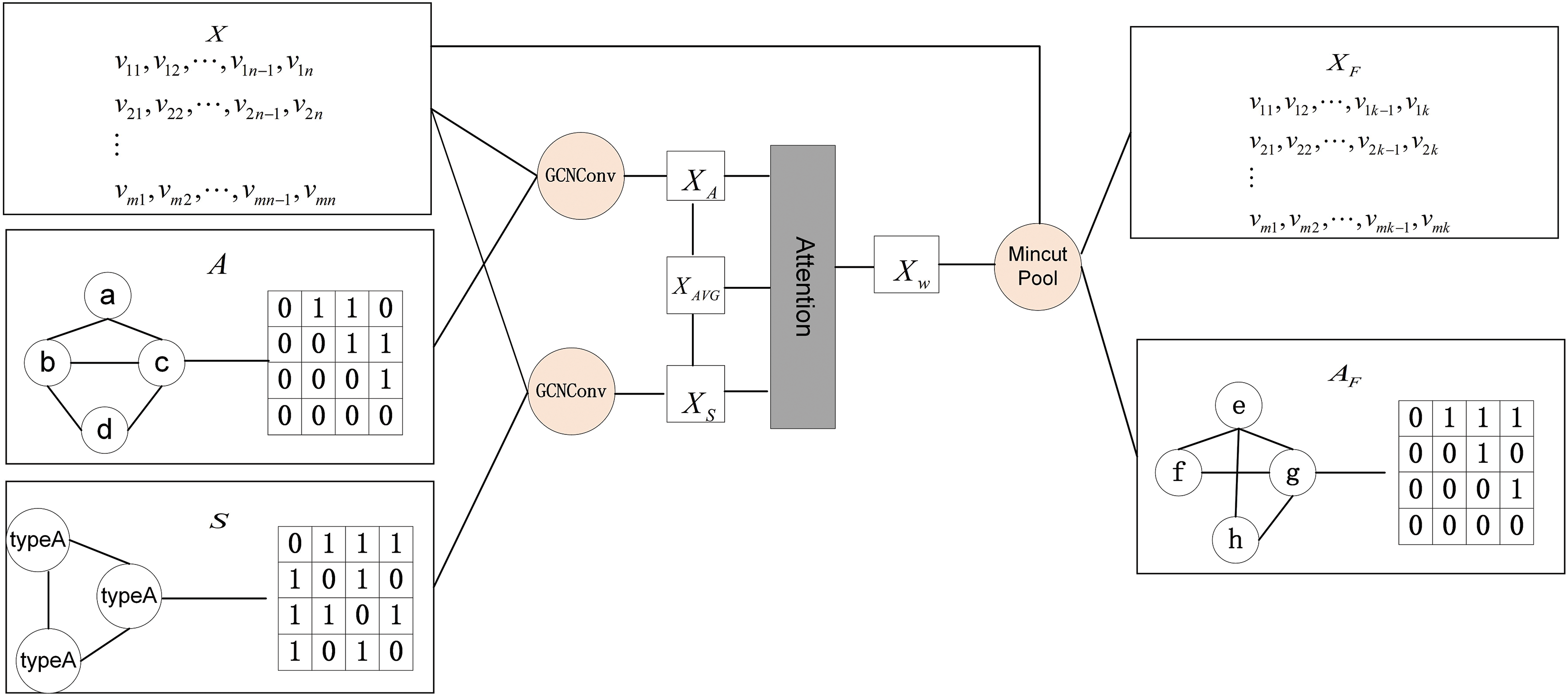
Figure 7: Graph convolutional neural network model based on neighborhood topology and spatial topology

XA=δ(D~A−12A~D~A−12XWA)(2)

A~=A+I(3)

XS=δ(D~S−12SD~S−12XWS)(4)

S~=S+I(5)

where A~ and S~ are the adjacency matrix and spatial identity matrix for adding self-connections, D~A and D~S are the degree matrices of A~ and S~, respectively, and WA and WS are the weight parameters to be learned. Secondly, we utilize the attention mechanism to adaptively learn the weight parameters of XA, XS and XAVG and obtain new node features XW. The specific realization formula is:

XAVG=XA+XS2(6)

Xw=w1XA+w2XS+w3XAVG(7)

Finally, by introducing the MinCutPool layer, the model realizes the downsampling of the graph, which not only drastically reduces the complexity of the subsequent computation, but also preserves the most important information in the graph structure.

In the second and third layers of the model, we continue to use the combination of GCN layer and MinCutPool layer to further analyze the graph structure data in depth. By halving the number of GCN channels layer by layer, the model is able to extract high-level abstract features in a more focused manner at each step. This hierarchical and progressive design idea not only improves the model’s ability to understand and capture the complex relationships in the graph structure, but also enables the model to comprehensively understand the structural and semantic properties of the code from both macro and micro levels.

3.2.2 Models for Handling Table-Structured Data

In the design of models that deal with structured data, this part of our model is used to process and analyze code dependency network (CDN) data and software metrics data. These data sources provide us with in-depth views of inter-code dependencies and metrics for static analysis of software code, which are key sources of information for understanding software quality and predicting potential defects. First, for the processing of code dependency network (CDN) data, we adopt a Zhang et al. [12] approach that combines a one-dimensional convolutional layer (CNN) and a bidirectional long- and short-term memory network (Bi-LSTM), and the structure of the model framework is shown in Fig. 8. The one-dimensional convolutional layer can effectively extract local features from CDN data and capture direct dependencies between code modules. Subsequently, by applying the bi-directional LSTM, the forward and backward bi-directional time series information is considered in the time dimension. This design allows the model to not only capture local dependency features between codes, but also analyze and understand code dependency data from a time series perspective.The CNN layer consists of a convolutional layer and a maximal pooling layer, which is used to process the input CDN dependency feature vector X, and is implemented as follows:

M=Conv1D(X)(8)

Oc=Maxpooling(M)(9)

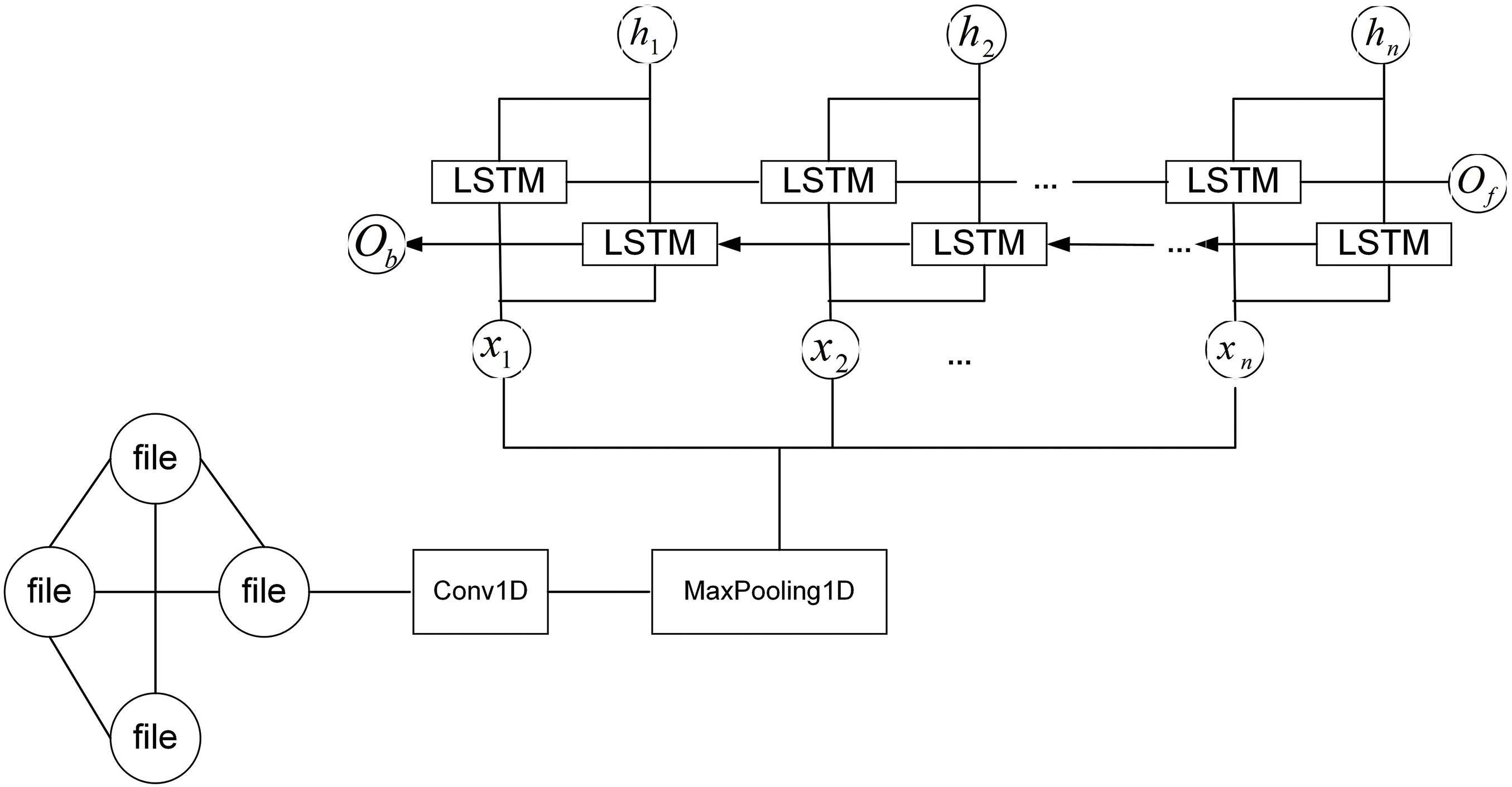
Figure 8: CNN1D-BiLSTM model

Bi-LSTM is used to process the output data of the CNN layer and selectively saves or deletes some information each time through three gate units, namely, oblivion gate, input gate, and output gate, which is realized by the following formula:

h→t=LSTM→(xt,ht−1→)(10)

ht=LSTM←(xt,ht−1←)(11)

Ht=[h→t;ht](12)

where h→t represents the forward hidden state of the time step t, ht represents the backward hidden state of the time step t, and Ht refers to the hidden state made by stitching h→t and ht together. The LSTM cell realization formula is as follows:

It=δ(XtWxi+Ht−1Whi+bi)(13)

Ft=δ(XtWxf+Ht−1Whf+bf)(14)

Ot=δ(XtWxo+Ht−1Who+bo)(15)

C~t=tanh⁡(XtWxc+Ht−1Whc+bc)(16)

Ct=Ft⊙Ct−1+It⊙C~t(17)

Ht=Ot⊙tanh⁡(Ct)+It⊙C~t(18)

where It is the input gate, Ft is the forgetting gate, Ot is the output gate, C~t is the candidate memory cell, Ct is the memory cell, W∗∗ and b∗ are the learning parameters, and ⊙ denotes dot product.

Second, for processing software static metric data we chose the TabNet classifier, which is a deep learning-based decision tree model designed for table-structured data. TabNet is able to efficiently distill the most critical information for software defect prediction from traditional metric data by learning to select the features that are most helpful for the prediction task. In the process, TabNet not only focuses on feature selection, but also further improves the model’s understanding and utilization efficiency of the data through feature transformation.

3.2.3 Feature Fusion and Defect Prediction

In this part, we fuse the features learned through GCN, CNN1D-BiLSTM and TabNet models by concatenating, and we downsize the features and predict whether the code is defective or not by using fully connected layer. In this paper, we train the prediction model by using binary cross-entropy loss function and Adam optimizer, in addition, in the defective dataset, there are more non-defective data than defective data, and we supplement the defective dataset by oversampling to make the two balanced.

4  Experiment

In this section, we show the experimental data of DP-MHHDL, the dataset used, the evaluation criteria, and the parameter settings. We also additionally selected six other models to complete the same experiments in the same setting to compare with DP-MHHDL.

All experiments were run on a machine with a GeForce RTX 2080 Ti with 10 cores and 16 GB GPUs, and the models were implemented on Tensorflow 2.4.0 using Keras2.4.

4.1 Datasets

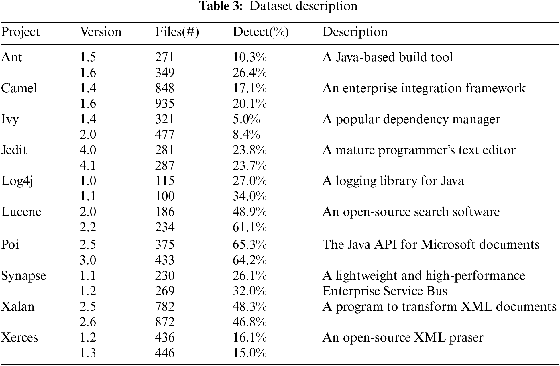
The datasets used in the experiments are from 10 open source projects in the promise database, which have different file counts, error rates, and development teams, and can well reflect the generality and practicality of our model. When performing defect prediction, we mainly perform cross-version defect prediction, i.e., we use earlier versions of the file code for generating the training set required for the experiment, and newer versions of the file code for generating the test set required for the experiment. The source codes of the projects were collected from github based on the name and version number of each project, and we also collected 20 metric features that reflect the project metric data and labels of whether the project is defective or not from github. The project details are shown in Table 3.

4.2 Evaluation Metrics

For this experiment we used F1 scores, auc scores and MCC to evaluate the performance of the model [22].

The F1 score balances the accuracy and recall of a classification model and is a weighted average of the model’s accuracy and recall.The value of the F1 score ranges from 0 to 1, with 0 indicating the worst performance and 1 indicating the best performance.The F1 score is defined as follows:

F1=2×precision×recallprecision+recall(19)

Precision=TPTP+FP(20)

Recall=TPTP+FN(21)

where TP is true positive, FP is false positive, FN is false negative and TN is true negative.

The Auc score is the area under the ROC curve, which can only be used for binary classification evaluation, and the larger its value, the more correct it is. It generally lies between 0.5 and 1, where 1 indicates the best performance and 0.5 indicates random prediction.

MCC is a metric for evaluating binary classification models for dealing with unbalanced data, which combines four metrics, TP, TN, FP and FN, and is more advantageous in the case of category imbalance and small sample size. It takes values between −1 and 1, where −1 means completely wrong, 0 means random prediction, and 1 means completely right, and MCC is defined as follows:

MCC=TP×TN−FP×FN(TP+FP)(TP+FN)(TN+FP)(TN+FN)(22)

4.3 Baseline Methods

In order to show the performance improvement of the DP-MHHDL, we have selected the following seven models as benchmark methods to compare with DP-MHHDL:

(1)   RF: Traditional metric data from the source code is trained by a Random Forest classifier.

(2)   Deep Belief Networks (DBN) [23]: AST is parsed from the source code, and the AST is parsed into a fixed-length vector using Word2Vec and then sent as input to the DBN model for defect prediction.

(3)   TabNet: traditional metric data from source code is trained by tabnet model.

(4)   Convolutional Graph Neural Network for Defect Prediction (DP-GCNN) [16]: Parsing AST from source code for defect prediction via an end-to-end model based on convolutional graph neural networks.

(5)   GH-LSTM [11]: The AST is parsed from the source code, and after parsing the AST into word vectors and the static metric data are inputted into the gated hierarchical long- and short-term memory network (GH-LSTM) model for defect prediction, respectively.

(6)   Hierarchical Feature Ensemble Deep Learning (HFEDL) [12]: Parsing AST, CDN, and traditional metrics data from source code, using these data as inputs to extract features from CNN and Bi-LSTM+Attention, and finally using an ensemble learning approach to integrate these sub-models into a final prediction model for defect prediction.

(7)   CGCN [24]: Abstract Syntax Trees (AST) and Class Dependency Network (CDN) are extracted from source code. The AST features are processed by CNN while CDN structure is learned through GCN. The fusion of AST semantic features and CDN structural information is then combined with traditional metrics for defect prediction.

4.4 Parameters Setting

The DP-MHHDL is implemented using the Keras deep learning library and Scikit-learn machine learning library. To ensure data balance, we divided all training sets into several batches, with each batch containing one positive and one negative data point. For the AST data input processing part, the vector dimension generated by one-hot encoding of AST node information is set to 39. The model accepting AST-related data input is graph convolutional neural network optimization model based on adjacency topology and spatial topology(ASGCN). Based on the research results of DP-GCNN, ASGCN consists of 3 layers of GCN model and pooling layer model. The input channel number of the first layer is the maximum number of AST nodes in the current project, and the input channel number of each subsequent layer is half of the previous layer, gradually reducing feature dimensions to extract more compact feature representations. All GCN layers use Relu as the activation function. For the CDN data input processing part, feature vectors are extracted through Node2Vec, with the feature vector dimension set to 50 (through experiments, we found that the model prediction performance is optimal when the dimension is 50). The model receiving CDN data input is the CNN1D-BiLSTM model. For CNN, the number of convolution kernels is 32, the length of convolution kernel is 1, and the activation function of the middle layer is Relu. For the BiLSTM model, the number of neurons is 8. For the traditional metric data input processing part, we performed normalization. The model receiving traditional metric data input is the TabNet model, which finds 16 optimal features among 20 dimensional feature columns, with a final output dimension of 16. Finally, the outputs of the three models are fused through fully connected layers, with ’sigmoid’ as the activation function of the output layer. Our model uses the Adam optimizer, with binary_crossentropy as the loss function, and 200 iterations for each project. The proposed method is evaluated in a cross-version context, where the previous version project is used as training data and the next version as test data. To avoid the impact of random errors on prediction results, each experiment is repeated 30 times, and the average is taken as the final prediction result.

The source code files and datasets used in the DP-MHHDL algorithm are publicly available on GitHub (https://github.com/feiqixia/DP-MHHDL) (accessed on 04 December 2024).

5  Result and Analysis

In this section, we test the performance of DP-MHHDL on specific datasets and compare it with other state-of-the-art software defect prediction models to reflect the validity and reasonableness of DP-MHHDL. Our results need to answer the following three questions:

RQ1: Does DP-MHHDL outperform other models that utilize a single data source to predict software defects?

RQ2: Does the performance of DP-MHHDL outperform other models that fuse multiple data to predict software defects?

RQ3: How do external parameters affect model performance?

5.1 Result and Analysis for RQ1

Tables 4–6 list the AUC, F1 and MCC scores for DP-MHHDL and for the four predictive software defect models that we compared using a single data source on different versions of the 10 datasets, where the best scores for the models are shown in red. Fig. 9 shows the data distribution of F1, AUC and MCC scores for different models in the form of box plots. Based on these graphs it can be seen that DP-MHHDL outperforms the other four models in terms of F1, AUC and MCC scores.

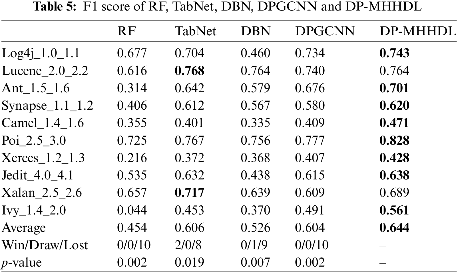
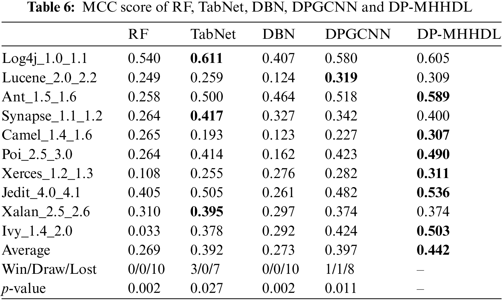
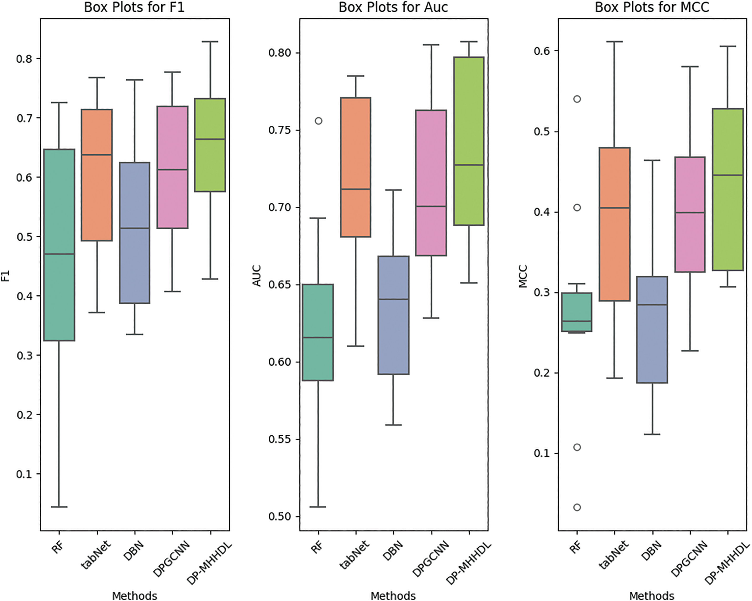
Figure 9: Box plots of prediction results compared with RF, TabNet, DBN, and DPGCNN models

(1)   From Tables 4–6, we can see that DP-MHHDL outperforms the other three models on all datasets except the TabNet model on all datasets except the lucene_2.0_2.2 dataset, and on average, DP-MHHDL outperforms RF, DBN, and DP-GCNN by 11, 10, and 2 percentage points on the AUC scores; by 19, 12, and 4 percentage points on the F1 scores; and by 18, 17, and 5 percentage points on the MCC scores. For the lucene project, DP-GCNN achieves the best results in terms of AUC and MCC scores, which are 0.6 and 1 percentage points higher than DP-MHHDL, respectively, but in terms of F1 scores, DP-MHHDL is 2 percentage points higher than DP-GCNN, which shows that DP-MHHDL has the same performance as DP-GCNN on lucene, while on all other datasets the model has to outperforms the other three models.

(2)   For the TabNet method, it was separated from DP-MHHDL and only the tabnet model was used to train the 20 traditional metrics on the data. As shown in Fig. 8, DP-MHHDL performs better in general than the TabNet method extracted alone. In Tables 4–6, specifically, DP-MHHDL achieves an advantage of 22 wins and 8 losses on all measures. It is worth noting that only on the xalan dataset does our model score worse than the TabNet method on all three measures, it is possible that the xalan dataset is the most balanced of all the datasets, and at this point fusing multiple inputs does not provide an advantage over training on a single data source. However, on the whole, DP-MHHDL, i.e., the model that fuses multiple inputs, outperforms the model that utilizes a single data source for prediction.

(3)   The Wilcoxon signed rank test is a nonparametric statistical test used to determine the difference between two methods. Usually, if the p-value of the Wilcoxon signed rank statistical test is less than 0.05, the difference between the two methods is considered to be significant, otherwise the difference is not significant, and DP-MHHDL shows significant improvement relative to the single-data-source defect prediction model under the F1, AUC, and MCC metrics (p < 0.05).

(4)   In addition, for the other models, it can be seen from Tables 4–6 and Fig. 9 that under the three measures of F1, AUC, and MCC, the TabNet model performs much better than RF, and the DP-GCNN scores much better than DBN. this also confirms that training the traditional metric data using the TabNet model is superior to RF, and for extracting the semantic features from the AST tree DP-GCNN is better than DBN. this confirms the validity and rationality of training traditional metric data and AST inputs in DP-MHHDL using TabNet model and DP-GCNN model, respectively.

In summary, based on the analysis of the experimental results, the effectiveness of the DP-MHHDL algorithm can be verified. The results show that extracting features from multiple information sources can significantly enhance the performance of defect prediction. This enhancement is attributed to the fact that our method not only incorporates traditional metric data, but also AST data and CDN data. Each of the three types of data reflects the code’s characteristic information from different dimensions, and by extracting and synthesizing features from these three types of data, a more comprehensive representation is constructed, which improves the effectiveness of defect prediction.

5.2 Result and Analysis for RQ2

Tables 7–9 list the F1, AUC, and MCC scores for DP-MHHDL and three other methods that incorporate multiple types of inputs, and Fig. 10 shows the distribution of data for these four methods in box-and-line plots. As shown in the box line plots and tabular data, our model outperforms GH-LSTM,HFEDL and CGCN.

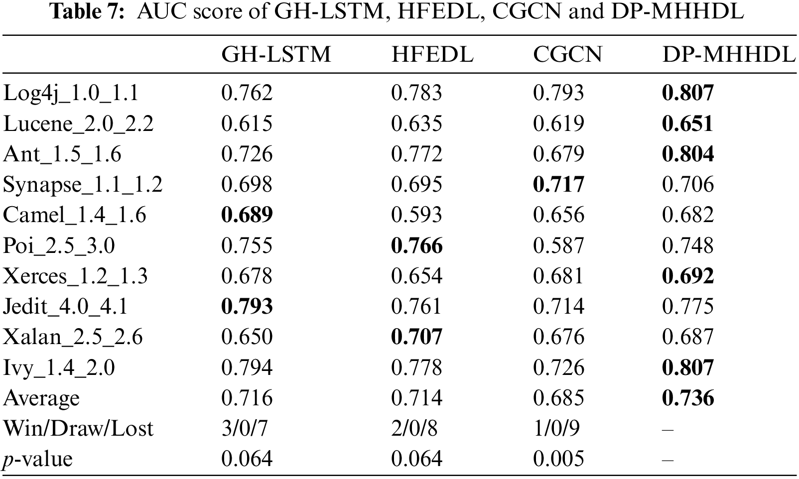
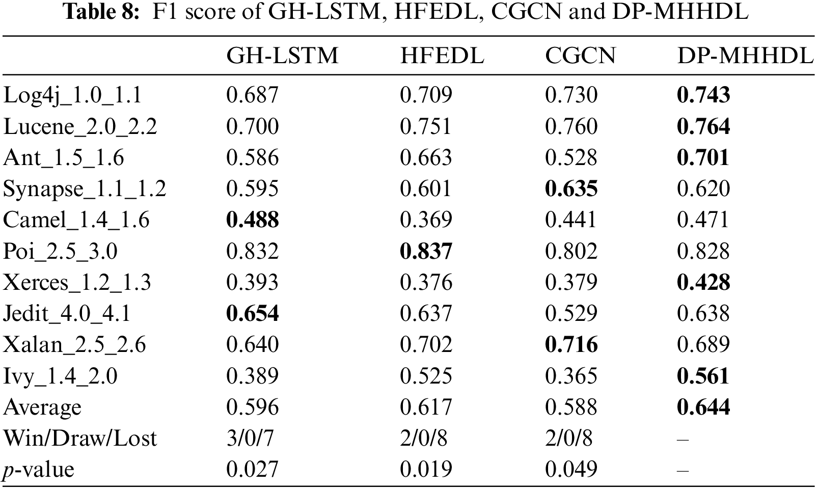
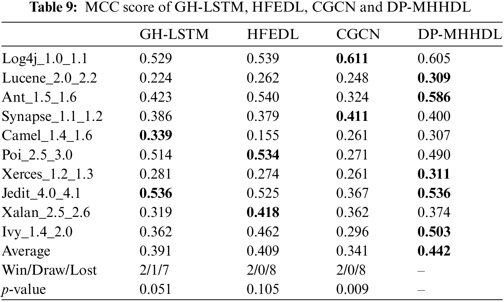
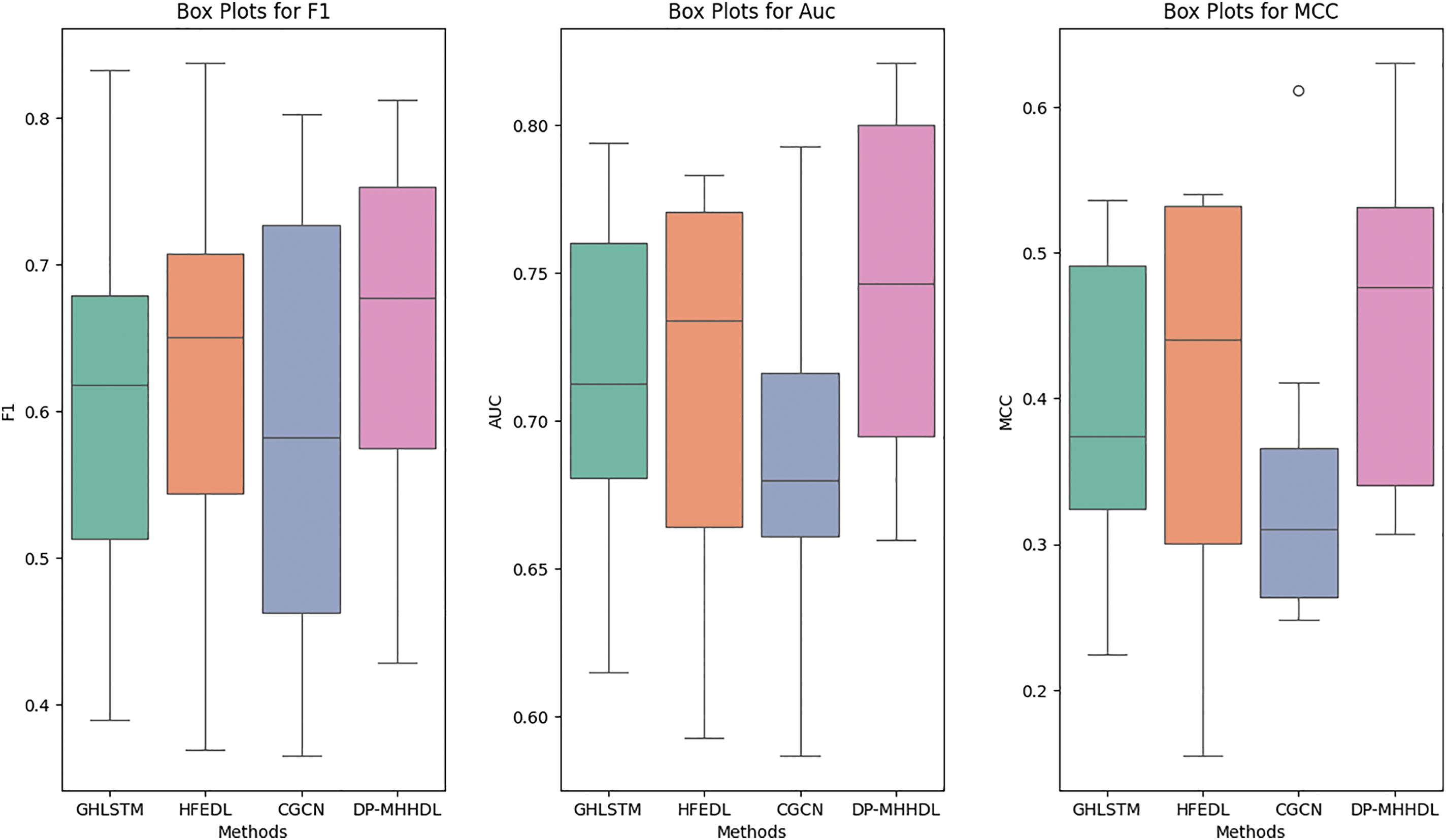
Figure 10: Box plots of prediction results compared with GH-LSTM, HFEDL and CGCN models

(1)   For the vast majority of the datasets in Tables 7–9, DP-MHHDL outperforms GH-LSTM, HFEDL and CGCN, with HFEDL achieving the best results only on the poi and xalan datasets, GH-LSTM having the three highest scores on the camel and jedit datasets and CGCN receiving the highest score on the dataset synapse. On average, DP-MHHDL is 2, 2 and 5 percentage points higher in AUC scores, 5, 3 and 6 percentage points higher in F1 scores, and 5, 4 and 10 percentage points higher in MCC scores compared to GH-LSTM, HFEDL and CGCN, respectively. It is clear from the box plots that both DP-MHHDL and the HFEDL model outperform the GH-LSTM, while DP-MHHDL significantly outperforms the HFEDL in terms of Auc and slightly outperforms the HFEDL in terms of F1 and MCC scores. The CGCN model, on the other hand, is more specific in that it performs the worst of the four models on the AUC and MCC scores, but comes close to the HFEDL and GH-LSTM on the F1 score. Overall, however, it performs worse than the DP-MHHDL on all three scores.

(2)   From the above analysis, we can see that DP-MHHDL is better than other fusion models in fusing multi-type input data. In addition, the performance of HFEDL is better than GH-LSTM, and HFEDL has more inputs of CDN type data than GH-LSTM in fusing the data, therefore, it is reasonable and effective for DP-MHHDL to add the inputs of CDN type data and train the CDN by using a similar model as HFEDL.

(3)   According to the statistical results and experimental analysis, DP-MHHDL showed significant improvement (p < 0.05) relative to CGCN. Under F1 metrics, DP-MHHDL shows significant improvement compared to GH-LSTM and HFEDL. Although in the measurement of MCC and AUC metrics, the p-value of our method with GH-LSTM and HFEDL algorithms is close to the significance level of 0.05 and fails to reach the significance threshold. However, considering the mean values of MCC and AUC and the Win/Draw/Lost statistics, our method still outperforms the GH-LSTM and HFEDL algorithms in terms of performance. Thus, our algorithm still demonstrates an overall advantage despite not reaching statistical significance in the p-values of the MCC and AUC metrics.

In summary, the experimental results show that constructing corresponding deep learning models for different data sources can extract richer and more comprehensive features than using the same deep learning model for all data sources, thus significantly improving the effectiveness of defect prediction. This improvement is due to the fact that the specific models designed for different data types (AST, CDN, and structured data) can better capture the feature information specific to the respective data, avoiding the limitations of a single model for multiple data sources. Meanwhile, the fusion strategy of the model effectively integrates the heterogeneous features of various types of data, which provides insights from multiple perspectives for defect prediction and enhances the generalization capability and prediction accuracy of the model.

5.3 Result and Analysis for RQ3

In this section, we first discuss the impact of the learning rate on the performance of the prediction model, and then, discuss how the word vector embedding dimension of the elements in a CDN affects the performance of the prediction method.

The setting of the learning rate is particularly important in the training of deep learning models. A learning rate that is too large will lead to an increase in the step size of the weight update, and the training results show a high degree of instability and may not converge to miss the optimal solution. A learning rate that is too small leads to a very small step size for weight update, slow training speed, and may fall into a local minimum of the loss function.

Bayesian optimization [25] It is an efficient global optimization algorithm that uses a Gaussian process to continuously update the prior values in order to find the optimal solution for the return value of the objective function. Bayesian optimization intelligently selects sampling points, reduces the number of evaluations to find the optimal solution, and can handle noisy data and uncertainty well.

In our experiments, we take Bayesian optimization to optimize the learning rate during model iterations. In each epoch, the Bayesian optimization method calculates the theoretical optimal learning rate of the current model. At the end of each epoch, we reset the learning rate of the current model to the optimal learning rate calculated by Bayesian optimization. The range of the Bayesian optimization learning rate was set to between 1e-6 and 1e-3, and to balance the three measures, the return value of the Bayesian optimization function we chose to be the reconciled mean of the normalized F1, AUC, and MCC scores.

In order to verify the advantages and effectiveness of Bayesian optimization, we tested the learning rate of 1e-4 and 1e-6 in the case of the environment and other hyper-parameters are exactly the same (the reason for not choosing 1e-3 is that for some datasets, the learning rate of 1e-3 is too large to lead to the model always fail to converge, and the data is not indicative), and the results of the test are shown in Figs. 11–13. As shown in the figures, the F1 scores under Bayesian conditioning outperform the other two learning rates for all items, and the AUC and MCC scores, except for the item poi, outperform the other two learning rates for the other items’ computed scores. On average, the F1, AUC and MCC scores under Bayesian parameterization are about 4 percentage points higher than the other two learning rates, while the F1, AUC and MCC scores computed when the learning rates are 1e-4 and 1e-6 do not differ much, which indicates that adjusting the value of the constant learning rate does not have much effect on the results of the prediction model, whereas using Bayesian optimization to dynamically change the learning rate in the learning process has a significant improvement.

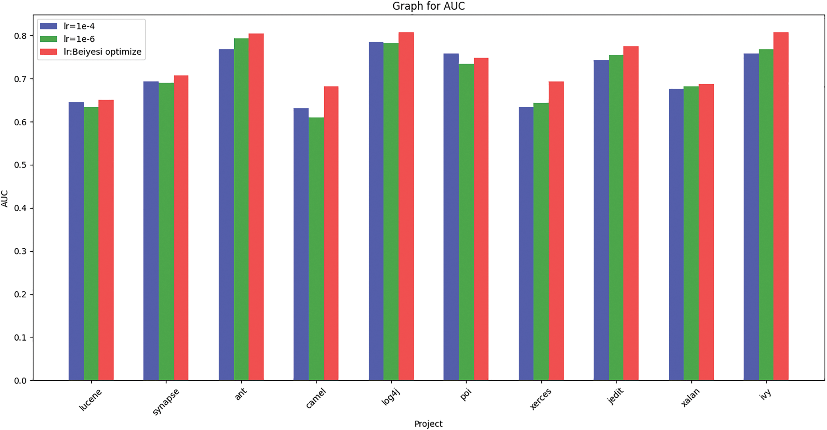
Figure 11: Histogram of AUC for different learning rates corresponding to different programs

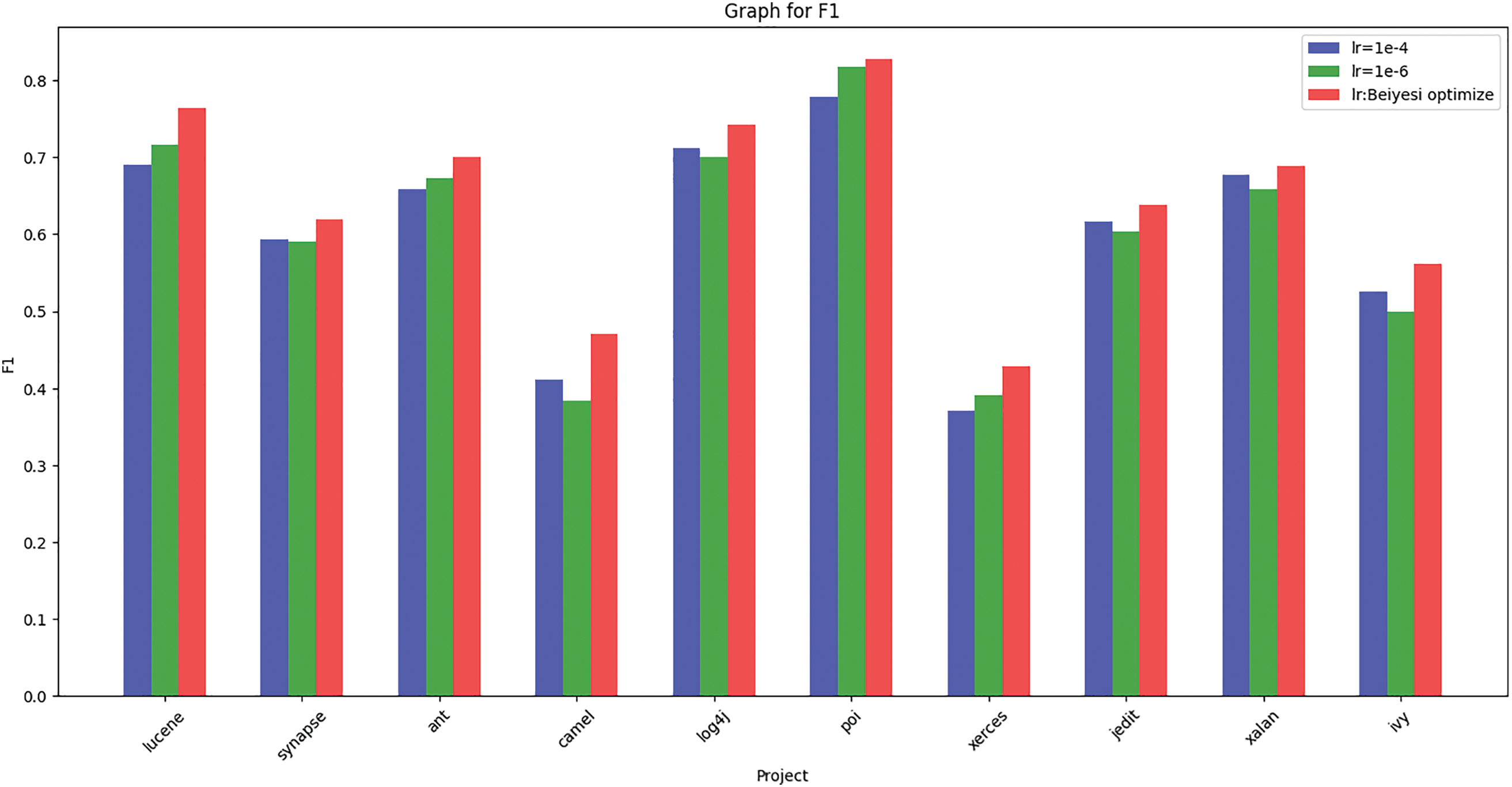
Figure 12: Histogram of F1 for different learning rates corresponding to different programs

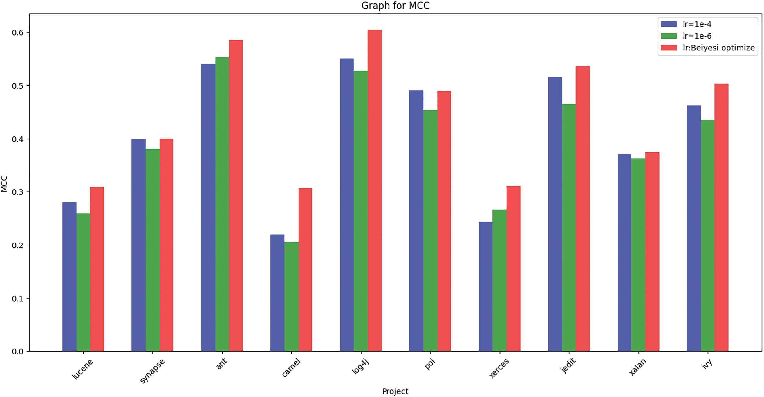
Figure 13: Histogram of MCC for different learning rates corresponding to different programs

In this paper, we use Node2Vec to extract feature vectors from CDN data, in order to investigate the effect of different vector dimensions on the prediction performance of the DP-MHHDL method. We set the dimensions to 10, 20, 30, 40, 50, and 60 sequentially and evaluate the prediction performance under these different dimensions. The experimental results are shown in Fig. 14, which illustrates the trend of the average prediction performance under each dimension over 10 experiments. It can be seen that the overall prediction performance maintains a relatively smooth trend as the dimensions change, and the prediction performance reaches a relative optimum when the vector dimension is set to 50. Therefore, the dimension is set to 50 in the CDN node word vector.

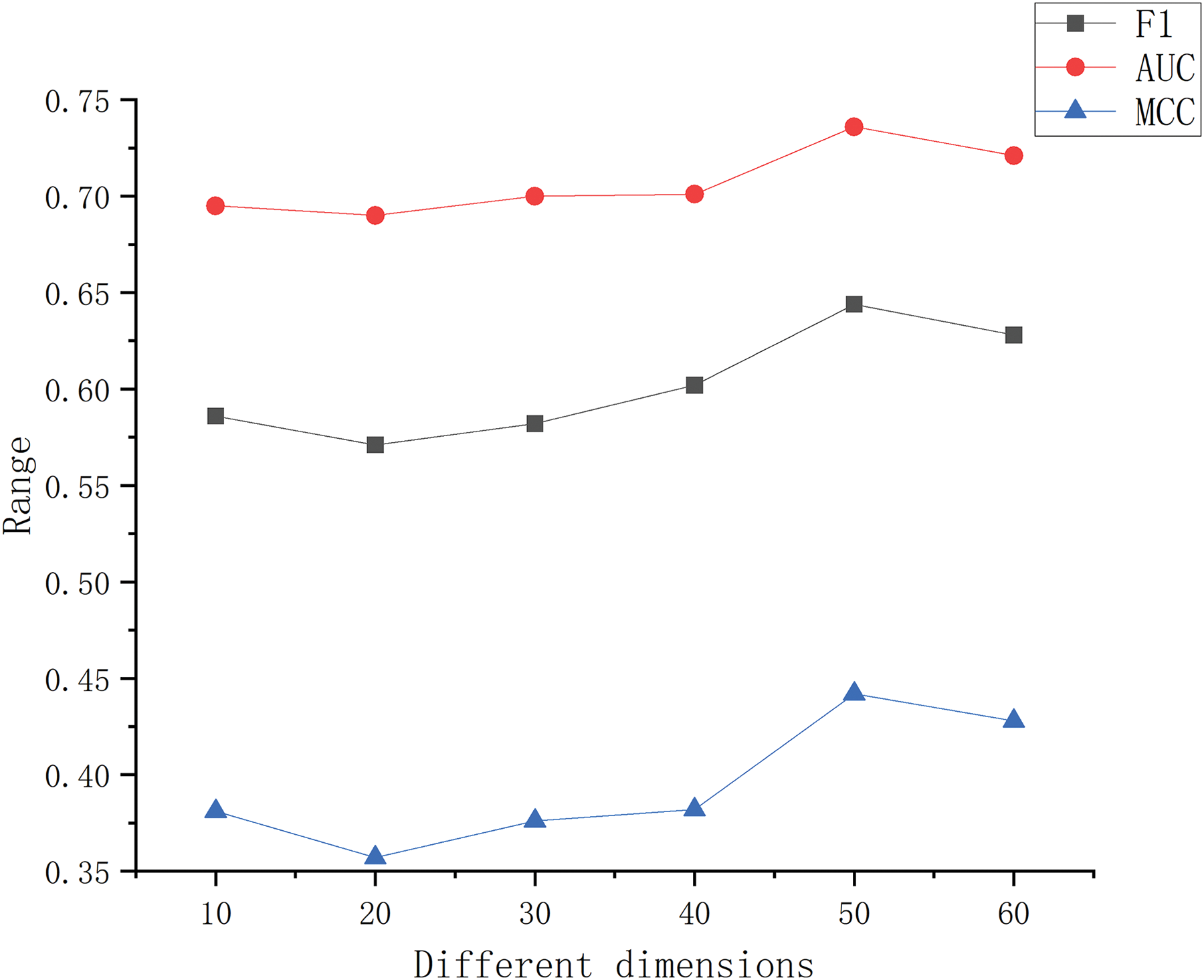
Figure 14: Predicted results for different embedding dimensions corresponding to the three metrics

6  Related Work

Traditional software defect prediction: For traditional metrics data, most of the earliest researchers used plain Bayes, Random Forest, and support vector machine algorithms. Okutan et al. [26] integrated 8 traditional static features to construct and analyze a Bayesian network from a dataset focusing on the dependencies between the metrics and their impact on software defects. The study conducted by Kaur et al. [27] conducted a study using Random Forest algorithm to predict error-prone software classes and they used the same 8 traditional static features. Elish’s [28] study used Support Vector Machines to learn predictions on 21 static features data extracted from source code and their results were also better than Random Forest and Bayes, which also proves that usually the more comprehensive static features obtained from a project are more beneficial to the accuracy of software defect prediction.

Abstract Syntax Tree in software defect prediction: Due to the lack of semantic information in traditional metric data, more and more work chooses to extract abstract syntax trees from the source code of a program and perform feature extraction and prediction by the rapidly developing deep learning models. Wang et al. [23] use Deep Belief Networks (DBNs) to extract semantic features from token vectors originating from the program’s Abstract Syntax Trees (ASTs) for a file-level defect prediction model, and from the source code changes for change-level defect prediction models. Li et al. [13] converted the acquired AST tree into an input for a CNN, which analyzed the code defect information embedded in the AST. Liang et al. [18] used LSTM to extract semantic information from the AST tree for defect prediction. Zhang et al. [29] used mapping and word embedding to convert the AST tree into a numeric vector, and extracted the information from it using a Transformer model to extract the syntactic and semantic features into a logistic regression classifier. Šilić et al. [16] converted the Abstract Syntax Tree (AST) of a software module into a graph representation, which was then processed by a GCNN to categorize the module as defective or non-defective. It can be seen that the models used to train the AST are becoming more and more complex, the semantic information extracted from them is becoming more and more complete, and the training results are superior to those of the previous simple models.

Extract features from multiple information sources: Given that extracting features from a single source of information cannot fully reflect the defects of the code, most of the current state-of-the-art methods extract features from multiple sources of information. Qu et al. [22] use Node2Vec to parse the CDN graph of a project into vectors and fuse the traditional features to input them into a traditional classifier for defect prediction. Zeng et al. [30] also use Node2Vec to parse the CDN graph of a project into vectors and fuse the traditional features, and process the fused features through a modified GCN model. Wang et al. [11] parsed the AST and traditional metrics data from the source code, and parsed the AST into word vectors and fed them into a hierarchical LSTM model for defect prediction. Fan et al. [31] extracted vector representations from ASTs, encoded them into numeric vectors through mapping and word embedding, and then used a recurrent neural network (RNN) to automatically learn semantic features from these numeric vectors and apply self-attention mechanisms to establish relationships between these features. Finally, these semantic features are combined with traditional static metrics to more accurately predict software defects.By integrating Abstract Syntax Trees (ASTs) and Control Flow Graphs (CFGs), Zhao et al. [32] relied on a graph attention mechanism to capture local features within code blocks and contextual features between different code blocks. Tao et al. [21] used a BiLSTM-based model to fuse features of the AST labeling sequence and code change tagging sequence features together to generate semantic features, and used a gated fusion mechanism to integrate these features with software metric data. Zhang et al. [12] parsed AST, CDN, and legacy metric data from the source code, extracted these data as inputs to extract features from CNNs and Bi-LSTM+Attention, and finally integrated these sub-models into the final LSTM model using an integrated learning approach to integrate these sub-models into the final prediction model for defect prediction.

Summary: From the existing studies, it can be seen that most of the current studies only extract features from a single information source or rely on a single deep learning model for defect prediction. Although this approach can capture some of the code features, the limitation of the information source and the singularity of the model lead to the one-sidedness of the extracted features in expressing the semantic complexity of the code, which affects the generalization ability and performance of the prediction model. In contrast, this paper proposes a more comprehensive solution that not only combines multiple deep learning models to automatically learn valuable features, but also enhances the performance of the model by extracting rich features from multiple information sources. Specifically, the approach in this paper incorporates multiple sources of information such as traditional metric data, AST abstract syntax trees and CDNs, and constructs different deep learning models TabNet, ASGCN, and CNN1D-BILSTM to process these features respectively, to fully explore the potential semantic features of various information sources. At the same time, we introduce an integrated learning approach to fuse the prediction results of multiple sub-models to improve the prediction performance of the overall model. This multi-model, multi-information source fusion strategy effectively overcomes the limitations of a single approach and can predict software defects more comprehensively and accurately. Compared with previous studies, the method in this paper not only has advantages in the comprehensiveness of feature extraction, but also substantially improves the accuracy and stability of prediction through multi-model integration. This provides a more prospective and practical solution for future software defect prediction in complex code environments.

7  Threats to Validity

7.1 Threats to Internal Validity

In this paper, we reproduce four other models as described in other papers and compare the results of these models with ours to demonstrate the validity and superiority of our model. However, even though we have completely built their models according to the descriptions of the papers, we still cannot guarantee that some parameter settings, method implementations, and environment configurations are exactly the same, which may affect the final results. Therefore, in order to fairly compare the performance of the models, each model is tested in the same environment, and other parameter settings and methods that are not mentioned in the paper are set to be the same as our model to ensure the validity of our model.

7.2 Threats to External Validity

In our experiments, we selected 10 projects from the promise open source library as datasets to evaluate the performance of our model. These 10 datasets are widely used in software defect prediction methods and have wide coverage, which is helpful in proving the effectiveness of our method. However, several limitations of the promise dataset may affect the generalizability of our results. First, since these projects are from older versions, they may not fully represent modern software development practices and contemporary defect patterns. Modern software systems often have different architectural patterns, coding standards, and complexity levels. Besides, the datasets mainly contain Java projects, which may limit the generalizability to other programming languages. Finally, the relatively small size of some projects in the dataset may not capture the complexity of large-scale industrial applications.

8  Conclusion and Future Work

Current software defect prediction research faces the challenge of failing to adequately consider the characteristics of different data sources either from a single data source or in real-world scenarios where multiple data sources coexist, and usually adopts a unified deep learning model for defect prediction. This approach ignores the variability among different data sources and their potential value, which may lead to limited accuracy and generalization performance of the prediction results. To this end, this paper proposes a multivariate heterogeneous hybrid deep learning algorithm (DP-MHHDL), which aims to fuse multivariate heterogeneous data to enhance the performance of software defect prediction. First, for the feature extraction of AST data, utilizing the advantages of GCN in processing graph-structured data, this paper proposes a deep learning model based on GCN (ASGCN), which is not only able to learn the semantic information in the context, but also able to capture the spatial feature information among similar nodes, which enhances the representation of graph-structured data. Second, although AST data retains the syntactic and semantic information of a single document, it cannot reflect the global importance of that document in the whole project. To solve this problem, this paper further integrates the features of CDN data and constructs the CNN1D-BiLSTM model based on LSTM’s ability to excel in capturing temporal features, which not only captures the temporal dependence of local features, but also improves the understanding of the temporal data, thus extracting the features of CDN data in a more comprehensive way. Finally, for feature extraction of traditional metric data, unlike other studies that use machine learning models such as Random Forest or SVM, this paper selects the TabNet model as a more suitable model for handling table-structured data for feature extraction. The experimental results show that TabNet has better results in processing defective metric data. To verify the superiority of the proposed algorithm, the performance of the algorithm is tested on 10 different datasets in this paper. The results show that the DP-MHHDL algorithm proposed in this paper achieves the optimal prediction results, both compared with the single data source model and the multi-data source fusion model.

In future work, we will further improve the data sources and models of our approach, consider adding control flow and data flow to AST to form code property graphs (CPG) to enhance the semantic features of the code, and adaptively select the optimal model and model structure and parameters via AutoML. Besides, we would like to utilize our method on C/C++ datasets if possible.

Acknowledgement: I express my sincere gratitude to all individuals who have contributed to this paper. Their dedication and insights have been invaluable in shaping the outcome of this work.

Funding Statement: The authors received no specific funding for this study.

Author Contributions: The authors confirm contribution to the paper as follows: study conception and design: Qi Fei, Haojun Hu; data collection: Qi Fei, Haojun Hu; analysis and interpretation of results: Qi Fei, Haojun Hu; draft manuscript preparation: Qi Fei, Haojun Hu, Guisheng Yin, Zhian Sun;manuscript final layout and preparation for submission: Qi Fei, Haojun Hu, Guisheng Yin, Zhian Sun. All authors reviewed the results and approved the final version of the manuscript.

Availability of Data and Materials: The source code files and datasets used in our DP-MHHDL algorithm are publicly available on GitHub (https://github.com/feiqixia/DP-MHHDL) (accessed on 24 October 2024).

Ethics Approval: Not applicable.

Conflicts of Interest: The authors declare no conflicts of interest to report regarding the present study.

References

1. D. Leffingwell and D. Widrig, Managing Software Requirements: A Use Case Approach, 2nd ed. USA: Addison-Wesley Professional, 2003. [Google Scholar]

2. S. Chidamber and C. Kemerer, “A metrics suite for object oriented design,” IEEE Trans. Softw. Eng., vol. 20, no. 6, pp. 476–493, 1994. doi: 10.1109/32.295895. [Google Scholar] [CrossRef]

3. T. McCabe, “A complexity measure,” IEEE Trans. Softw. Eng., vol. 2, no. 4, pp. 308–320, 1976. doi: 10.1109/TSE.1976.233837. [Google Scholar] [CrossRef]

4. M. H. Halstead, Elements of Software Science (Operating and Programming Systems Series). USA: Elsevier Science Inc., 1977. [Google Scholar]

5. L. Qiong Chen, C. Wang, and S. Song, “Software defect prediction based on nested-stacking and heterogeneous feature selection,” Compl. Intell. Syst., vol. 8, pp. 3333–3348, 2022. [Google Scholar]

6. Z. M. Zain, S. Sakri, N. H. A. R. Ismail, and R. M. Parizi, “Software defect prediction harnessing on multi 1-dimensional convolutional neural network structure,” Comput. Mater. Contin., vol. 71, no. 1, pp. 1521–1546, 2022. doi: 10.32604/cmc.2022.022085. [Google Scholar] [CrossRef]

7. N. A. A. Khleel and K. Nehéz, “A novel approach for software defect prediction using CNN and GRU based on SMOTE tomek method,” J. Intell. Inf. Syst., vol. 60, no. 3, pp. 673–707, May 2023. doi: 10.1007/s10844-023-00793-1. [Google Scholar] [CrossRef]

8. A. B. Farid, E. M. Fathy, A. Sharaf Eldin, and L. A. Abd-Elmegid, “Software defect prediction using hybrid model (CBIL) of convolutional neural network (CNN) and bidirectional long short-term memory (Bi-LSTM),” PeerJ. Comput. Sci., vol. 7, 2021, Art. no. e739. doi: 10.7717/peerj-cs.739. [Google Scholar] [PubMed] [CrossRef]

9. K. H. Dam et al., “A deep tree-based model for software defect prediction,” 2018, arXiv:1802.00921. [Google Scholar]

10. G. Fan, X. Diao, H. Yu, K. Yang, L. Chen and A. Vitiello, “Software defect prediction via attention-based recurrent neural network,” Sci. Program., vol. 2019, no. 1, pp. 1–14, Jan 2019. doi: 10.1155/2019/6230953. [Google Scholar] [CrossRef]

11. H. Wang, W. Zhuang, and X. Zhang, “Software defect prediction based on gated hierarchical lstms,” IEEE Trans. Reliab., vol. 70, no. 2, pp. 711–727, 2021. doi: 10.1109/TR.2020.3047396. [Google Scholar] [CrossRef]

12. S. Zhang, S. Jiang, and Y. Yan, “A hierarchical feature ensemble deep learning approach for software defect prediction,” Int. J. Softw. Eng. Knowl. Eng., vol. 33, no. 04, pp. 543–573, 2023. doi: 10.1142/S0218194023500079. [Google Scholar] [CrossRef]

13. J. Li, P. He, J. Zhu, and M. R. Lyu, “Software defect prediction via convolutional neural network,” in 2017 IEEE Int. Conf. Softw. Qual., Reliab. Secur. (QRS), 2017, pp. 318–328. [Google Scholar]

14. S. Hochreiter and J. Schmidhuber, “Long short-term memory,” Neural Comput., vol. 9, no. 8, pp. 1735–1780, 1997. doi: 10.1162/neco.1997.9.8.1735. [Google Scholar] [PubMed] [CrossRef]

15. J. Deng, L. Lu, and S. Qiu, “Software defect prediction via LSTM,” IET Softw., vol. 14, no. 4, pp. 443–450, Aug 2020. doi: 10.1049/iet-sen.2019.0149. [Google Scholar] [CrossRef]

16. L. Šikić, A. S. Kurdija, K. Vladimir, and M. Šilić, “Graph neural network for source code defect prediction,” IEEE Access, vol. 10, no. 1, pp. 10 402–10 415, 2022. doi: 10.1109/ACCESS.2022.3144598. [Google Scholar] [CrossRef]

17. S.Ã. Arik and T. Pfister, “TabNet: Attentive interpretable tabular learning,” Proc. AAAI Conf. Artif. Intell., vol. 35, no. 8, pp. 6679–6687, May 2021. doi: 10.1609/aaai.v35i8.16826. [Google Scholar] [CrossRef]

18. H. Liang, Y. Yu, L. Jiang, and Z. Xie, “Seml: A semantic LSTM model for software defect prediction,” IEEE Access, vol. 7, pp. 83 812–83 824, 2019. doi: 10.1109/ACCESS.2019.2925313. [Google Scholar] [CrossRef]

19. A. K. Jakhar and K. Rajnish, “Software fault prediction with data mining techniques by using feature selection based models,” Int. J. Electr. Eng. Inform., vol. 10, no. 3, pp. 447–465, 2018. doi: 10.15676/ijeei.2018.10.3.3. [Google Scholar] [CrossRef]

20. R. R. Kumar and A. Chaturvedi, “Software fault prediction using data mining techniques on software metrics,” in Machine Learning and Big Data Analytics. Cham: Springer, 2021. doi: 10.1007/978-3-030-82469-3_27. [Google Scholar] [CrossRef]

21. C. Tao, T. Wang, H. Guo, and J. Zhang, “An approach to software defect prediction combining semantic features and code changes,” Int. J. Softw. Eng. Knowl. Eng., vol. 32, no. 09, pp. 1345–1368, 2022. doi: 10.1142/S0218194022500504. [Google Scholar] [CrossRef]

22. Y. Qu and H. Yin, “Evaluating network embedding techniques’ performances in software bug prediction,” Empirical Softw. Engg., vol. 26, no. 4, Jul. 2021. doi: 10.1007/s10664-021-09965-5. [Google Scholar] [CrossRef]

23. S. Wang, T. Liu, J. Nam, and L. Tan, “Deep semantic feature learning for software defect prediction,” IEEE Trans. Softw. Eng., vol. 46, no. 12, pp. 1267–1293, 2020. doi: 10.1109/TSE.2018.2877612. [Google Scholar] [CrossRef]

24. C. Zhou, P. He, C. Zeng, and J. Ma, “Software defect prediction with semantic and structural information of codes based on graph neural networks,” Inf. Softw. Tech., vol. 152, 2022, Art. no. 107057. doi: 10.1016/j.infsof.2022.107057. [Google Scholar] [CrossRef]

25. J. Snoek, H. Larochelle, and R. P. Adams, “Practical bayesian optimization of machine learning algorithms,” in Proc. 26th Annu. Conf. Neural Inform. Process. Syst., Lake Tahoe, NV, USA, Curran Associates Inc., 2012, pp. 2951–2959. [Google Scholar]

26. A. Okutan, “Software defect prediction using bayesian networks,” Empir. Softw. Eng., vol. 19, no. 1, pp. 154–181, 2014. doi: 10.1007/s10664-012-9218-8. [Google Scholar] [CrossRef]

27. A. Kaur and R. Malhotra, “Application of random forest in predicting fault-prone classes,” in 2008 Int. Conf. Adv. Comput. Theo. Eng., 2008, pp. 37–43. [Google Scholar]

28. K. O. Elish and M. O. Elish, “Predicting defect-prone software modules using support vector machines,” J. Syst. Softw., vol. 81, no. 5, pp. 649–660, 2008. doi: 10.1016/j.jss.2007.07.040. [Google Scholar] [CrossRef]

29. Q. Zhang and B. Wu, “Software defect prediction via transformer,” in 2020 IEEE 4th Inform. Technol., Netw., Electr. Automat. Cont. Conf. (ITNEC), 2020, vol. 1, pp. 874–879. doi: 10.1109/ITNEC48623.2020. [Google Scholar] [CrossRef]

30. C. Zeng, C. Y. Zhou, S. K. Lv, P. He, and J. Huang, “GCN2defect: Graph convolutional networks for smotetomek-based software defect prediction,” in 2021 IEEE 32nd Int. Symp. Softw. Reliab. Eng. (ISSRE), 2021, pp. 69–79. [Google Scholar]

31. G. Fan, X. Diao, H. Yu, K. Yang, and L. Chen, “Deep semantic feature learning with embedded static metrics for software defect prediction,” in 2019 26th Asia-Pacific Softw. Eng. Conf. (APSEC), 2019, pp. 244–251. [Google Scholar]

32. Z. Zhao, B. Yang, G. Li, H. Liu, and Z. Jin, “Precise learning of source code contextual semantics via hierarchical dependence structure and graph attention networks,” J. Syst. Softw., vol. 184, 2022, Art. no. 111108. doi: 10.1016/j.jss.2021.111108. [Google Scholar] [CrossRef]