TMC-GCN: Encrypted Traffic Mapping Classification Method Based on Graph Convolutional Networks

1  Introduction

Identifying and classifying network traffic is essential for applications such as QoS, pricing, and security measures, including malware and intrusion detection [1]. Using encryption to protect data transmissions enhances user privacy [2], but also complicates traffic classification, as it allows malware and cybercriminals to evade detection through tools such as Tor and VPNs. Moreover, owing to the diversity of applications, the granularity of today’s traffic classification is becoming increasingly fine, and an increasing number of traffic types must be distinguished by traffic classifiers. The most popular method is the deep-learning-based encrypted traffic classification model.

Deep-learning-based methods for encrypted traffic classification, such as Convolutional Neural Networks (CNN) [3,4] and Recurrent Neural Networks (RNN) [5], have shown promise [6–8]. Unlike traditional machine learning, deep learning automatically extracts features from raw data and uses an end-to-end learning approach, which avoids manual feature engineering and subdivision problems such as feature selection. However, these methods often process traffic characteristics independently, overlook packet relations, and lack a holistic network view, which can compromise the system’s robustness and practical application.

Mapping the relationship between packets in the traffic into a topology structure, using the topology structure to map to the non-Euclidean space to save packet information [9], and using a Graph Neural Network (GNN) to process the data of this network topology can solve the above problems. Originally developed by Scarselli et al. [10], GNNS was later refined by Scarselli et al. and Micheli et al. Early GNN models used RNNs to extend the CNN framework to graph-structured data, leading to the creation of Graph Convolutional Networks (GCN) and their variants [11], which advanced deep-learning applications on graph data. Shen et al. [12] introduced a Traffic Interaction Graph (TIG), where vertices represent packets with directions, edges represent packet-level interactions between clients and servers, and connections between adjacent bursts [13]. Jiang et al. [14] developed a Flow-level Relation Graph (FRG) to represent traffic data that preserves packet-level details, such as size, direction, and time interval, as well as the edges of concurrent and triggered interactions between bursts. However, TIG and FRG ignore the relationship between packets in the same direction. Ignoring these relationships means that the full characteristics of the communication patterns may not be fully captured, thus affecting the accuracy of traffic classification and analysis.

To solve the above problems, this study proposes an FMG for network traffic that enhances the relationship between packets by mapping the relationship between adjacent packets and packets in the same direction as a network topology structure graph, thereby enhancing the understanding of internal flows and continuous packet sequences. The TMC-GCN designed in this study uses an FMG to map traffic data and capture the complex relationship of dimensions, such as order, time, and content, to enhance model classification and prediction ability. This approach also helps to quickly analyze client-side request-response sequences and server-side response patterns, such as bursts of traffic. The main contributions of this study are as follows:

(1) A network topology graph of the traffic is constructed. In an FMG, vertices represent packets, and edges represent the associations between packets. Sequential edges describe the temporal relationship of data packets, and jump-order edges are the key to this method. Jump-order edges capture the relationship of packets in bursts in the same direction as the flow and provide a finer and more comprehensive representation of the interaction of vertexes.

(2) A TMC-GCN model is designed that combines a GCN with a Multi-Layer Perceptron (MLP) to effectively learn vertex features and their structural relationships in a FMG. The GCN layer utilizes adjacency information to capture the relationships between vertices connected by sequential and jump-order edges, whereas the MLP applies nonlinear transformations to project features to a higher level of abstract feature space.

(3) To test the interpretability of FMG, other classical models were compared with the TMC-GCN model: CICAAGM2017 [15], CICIOT2023 [16], GraphDapp [12], and ISCXVPN2016 [17]. The accuracy of the experimental results ranged from 93%–98%.

The remainder of this paper is organized as follows. Section 2 summarizes related work, Section 3 presents the construction of the FMG and the design details of the TMC-GCN, Section 4 presents the performance tests and experiments of the FMG effectiveness evaluation, and Section 5 concludes the paper.

2  Related Work

Currently, most methods used in encrypted traffic classification are based on deep learning and graph neural network area types of deep learning. Therefore, this section introduces the encrypted traffic classification technology of traditional deep learning and the encrypted traffic classification technology of deep learning based on a graph neural network.

2.1 Classification of Encrypted Traffic Based on Deep Learning

Deep learning techniques that automatically extract features from raw data and utilize an end-to-end learning approach are highly effective for traffic classification tasks [18]. For example, Liu et al. introduced FS-Net [19], using packet-length sequences and a bidirectional Gated Recurrent Unit (GRU) [20] with a reconstruction autoencoder for encrypted traffic classification. Aceto et al. developed MIMETIC [21], a multimodal deep learning model using a CNN and a GRU for mobile-encrypted traffic analysis. Shapira et al. proposed FlowPic [22], which converts flow data into images for CNN-based classification. Wang et al. introduced the App-Net model [23] by employing Long Short-Term Memory (LSTM) and a CNN to analyze packet lengths and payload sequences. Liu et al. designed the BGRUA model [24] that uses a bidirectional GRU with an attention mechanism for HTTPS traffic analysis. Lin et al. developed ET-BERT [25], a transformer-based model that pretrains traffic data to understand the contextual relationships and transmission sequences. Lotfollahi et al. [26] proposed a deep learning-based method for encrypted traffic classification called “Deep Packet.” This method utilizes two deep neural network architectures, the Stack Autoencoder (SAE) and CNN, for application identification.

However, these deep-learning methods generally use statistical features or raw bytes directly to represent network traffic, adopt various learning models, and ignore the lack of inherent translation invariance of non-Euclidean traffic data. Ordinary deep learning models map network traffic into Euclidean space, thereby losing important information from packet relationships. GNN can be used to address this problem. A GNN can compose traffic data and use a graph structure to reflect the relationship between packets in the traffic data or the relationship between bytes in the packet. This relationship often intersects multiple dimensions, such as order, time, and content, forming complex connections. A GNN can effectively capture and learn complex relationships and enhance the classification and prediction abilities of a model.

2.2 Classification of Encrypted Traffic Based on Graph Neural Networks

GNNs have been effectively applied across various fields, particularly in handling un-structured data. Pang et al. [27] introduced CGNN, a chained graph model for maintaining sequences in traffic analysis. Zheng et al. [28] developed GCNETA, a GCN-based method for malicious traffic detection that combines statistical and structural network data to enhance accuracy. Huoh et al. [29] utilized a GNN for encrypted flow classification by analyzing packet relationships. Diao et al. [30] created EC-GCN, a framework using a multi-scale GCN to classify encrypted traffic. Shen et al. [12] developed GraphDApp, which uses a TIG for identifying traffic from distributed applications by treating it as a graph classification challenge. Jiang et al. [14] proposed FG-Net, employing an FRG graph structure to approach mobile encrypted traffic fingerprinting as a graph representation learning task.

However, traffic classification methods based on graph neural networks ignore the relationships between packets in the same direction. To this end, the FMG designed in this study strengthens the connection between these same-direction bursts or data packets, enabling rapid location and analysis of situations where the client sends consecutive requests, as well as the degree of correlation between these request responses. The data packets are represented as vertices with directions by constructing separate graphs for each flow. Sequential edges were used to represent the time–sequence relationship of the data packets in the network flow, and jump-sequence edges were used to represent the burden relationship in the same direction in the flow. Then, the GCN and MLP are used to learn the graph, which can achieve good classification results.

3  TMC-GCN Model Construction

3.1 Construction of the Flow Mapping Graph

Several steps are required before building an FMG: (1) First, data packets from different applications must be collected. When a client visits software or a website, all the recorded network traffic consists of packets transmitted across multiple sessions. (2) These raw data are classified into independent flows according to the principle of sharing the same quintuple (source and destination IP addresses, source and destination port numbers, and protocols), where each flow consists of a series of data packets with the same quintuple. Consider the interactive process shown in Fig. 1, where the number represents the packet length with direction, and the sequence can be expressed as “packet length”: [193, −1338, −1338, −857, 126, 51, 494, −463, −251, 31, 38]. A positive number represents a packet sent from the client to the server, whereas a negative number represents a packet sent to the client.

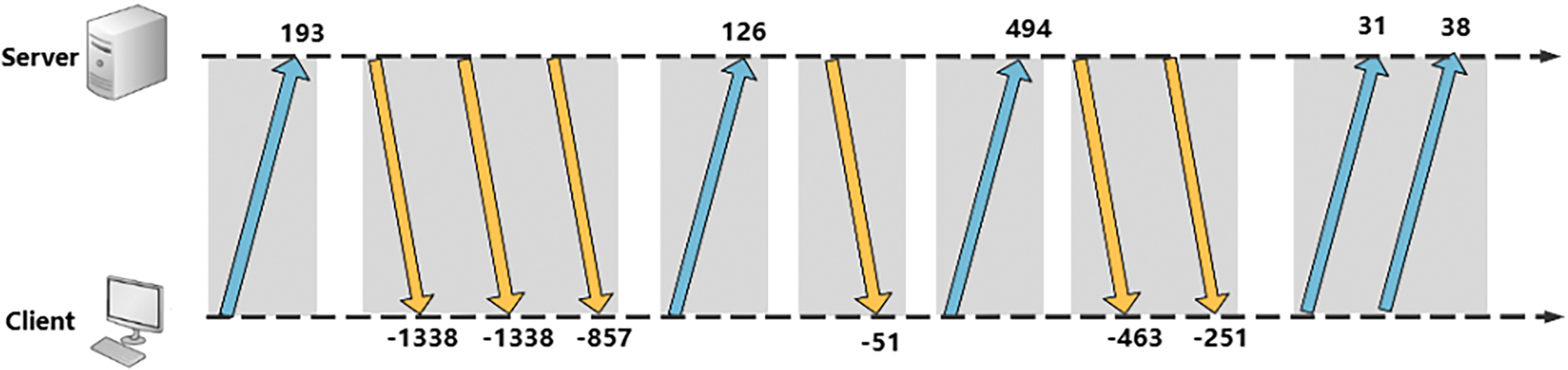
Figure 1: Example of packet-level client-server interaction for a stream

FMG represents the graph structure of each flow, which can be represented by a vector of common flow packet lengths consisting of n packets. Flow=f1,f2,…,fn, where fi indicates the first i with symbols of the length of the packet, and the FMG construction process is as follows:

Vertex: In an FMG, each packet in a stream corresponds to a vertex linked to the packet’s length, with the direction indicated by a positive or negative value. For example, Flow = [193, −1338, −1338, −857, 126, −51, 494, −463, −251, 31, 38] represents a sequence of 11 packets, as shown in Table 1, where each packet is a vertex in the FMG. Consecutive packets in the same direction form a burst “[13]”, even if they are single packets. Seven bursts occurred in the given flow {193}, {−1338, −1338, −857}, {126}, {−51}, {494}, {−463, −251}, {31, 38}. To avoid FMG complexity and maintain the TMC-GCN performance and time efficiency, only the first 160 packets in each flow were selected as vertices for the reasons detailed in Section 4.

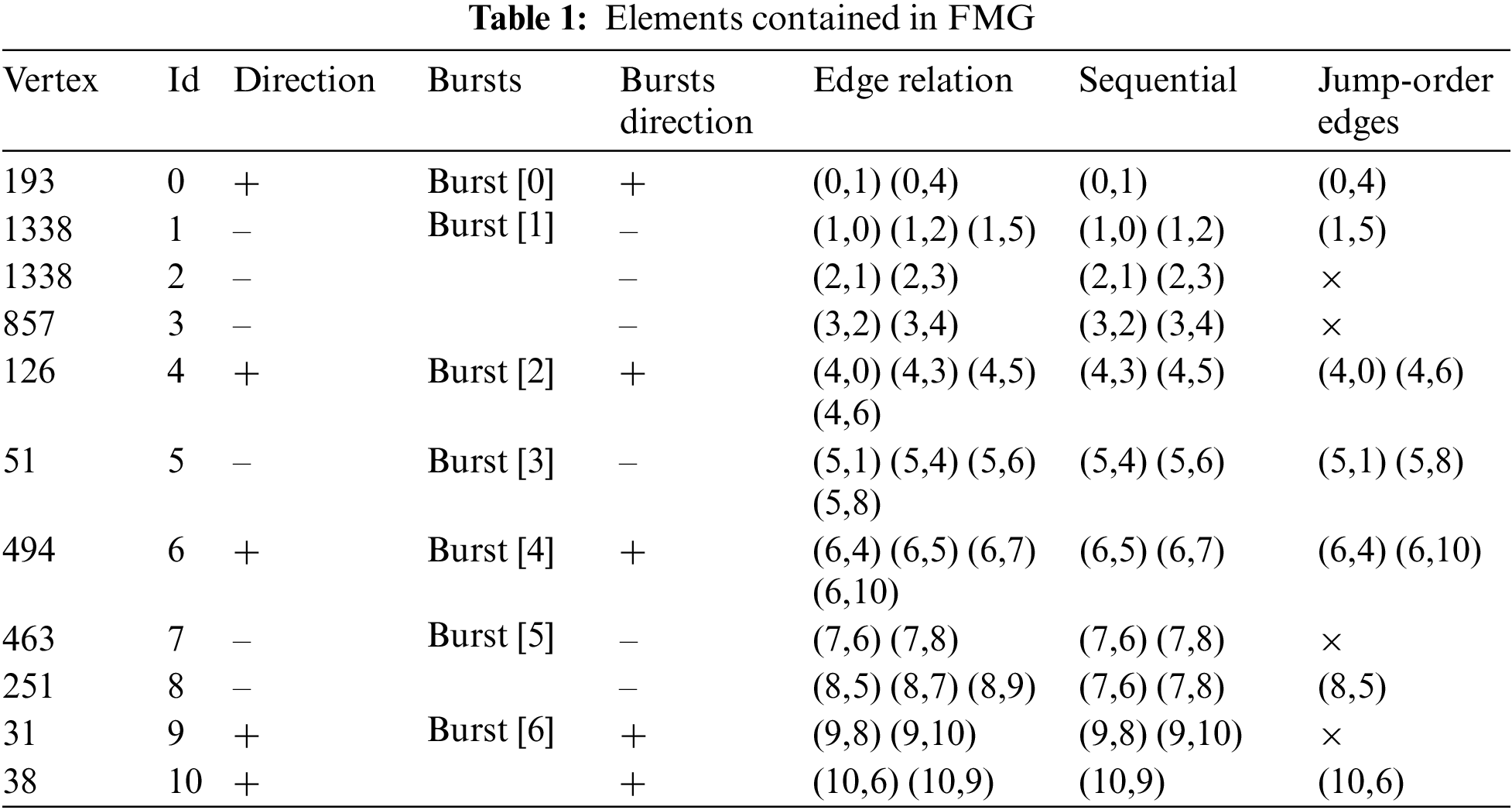
Edges: Edges in the graph representing connections between vertices significantly influence the feature aggregation. The graph structure included sequential and jump-order edges. (1) Sequential edges: Packets are sorted by arrival timestamps, with each packet length treated as a vertex. These vertices are then connected to form n−1 sequential edges. The construction of sequential edges reflects the timing characteristics of packets. (2) Jump-order edges: The packets are classified into bursts based on their direction and continuity. The last vertex of the same-direction burst is connected to the first vertex of the continuous same-direction burst, forming a jump-order edge. Communication characteristics between client and server, such as request and response patterns, persistent connection state, and directionality of data transfer, are important to define bursty head and tail connections in FMG. For example: Persistent connection states: such as FTP or database connections, usually involve multiple consecutive bursts of data exchange, and these bursts of connection help reveal the nature of the whole session. Data transfer direction: Upload and download activities are clearly different in direction, and this directional change can be reflected in FMG by the jump-order edges. In network communication, data flows in the same direction often have specific intentions or functions (such as file transfer, video streaming, etc.), and the model can better capture this pattern by jump-order edges. When dealing with complex network traffic, it is difficult to get effective information from only a single data packet. Jump-order edges provide a mechanism to exploit contextual information by connecting relevant bursts, thus improving the accuracy of recognition and classification. For instance, in Fig. 1, the vertex of a single burst {−51} is linked to the first vertex (−1338) of the prior same-direction burst {−1338, −1338, −857}, and the first vertex (31) of burst {31, 38} is linked to vertex (494) of the previous same-direction burst {494}. Fig. 2a,b shows the structure of sequential edge and jump-order edge respectively, and Fig. 2c is the final FMG structure, where the line represents the sequential edge and the dashed line represents the jump-order edge. The edge relation in Table 1 shows the specific edge connections with numbered vertices. All edges in FMG are undirected, allowing bidirectional information exchange in the neural network for more comprehensive vertex feature aggregation.

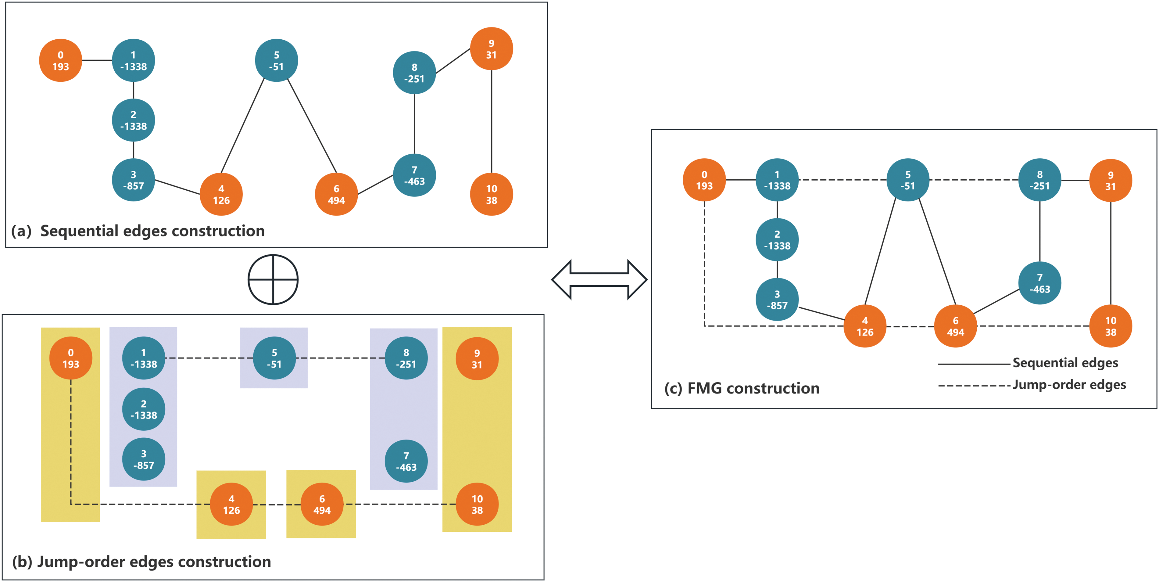
Figure 2: FMG construction process for encrypted traffic

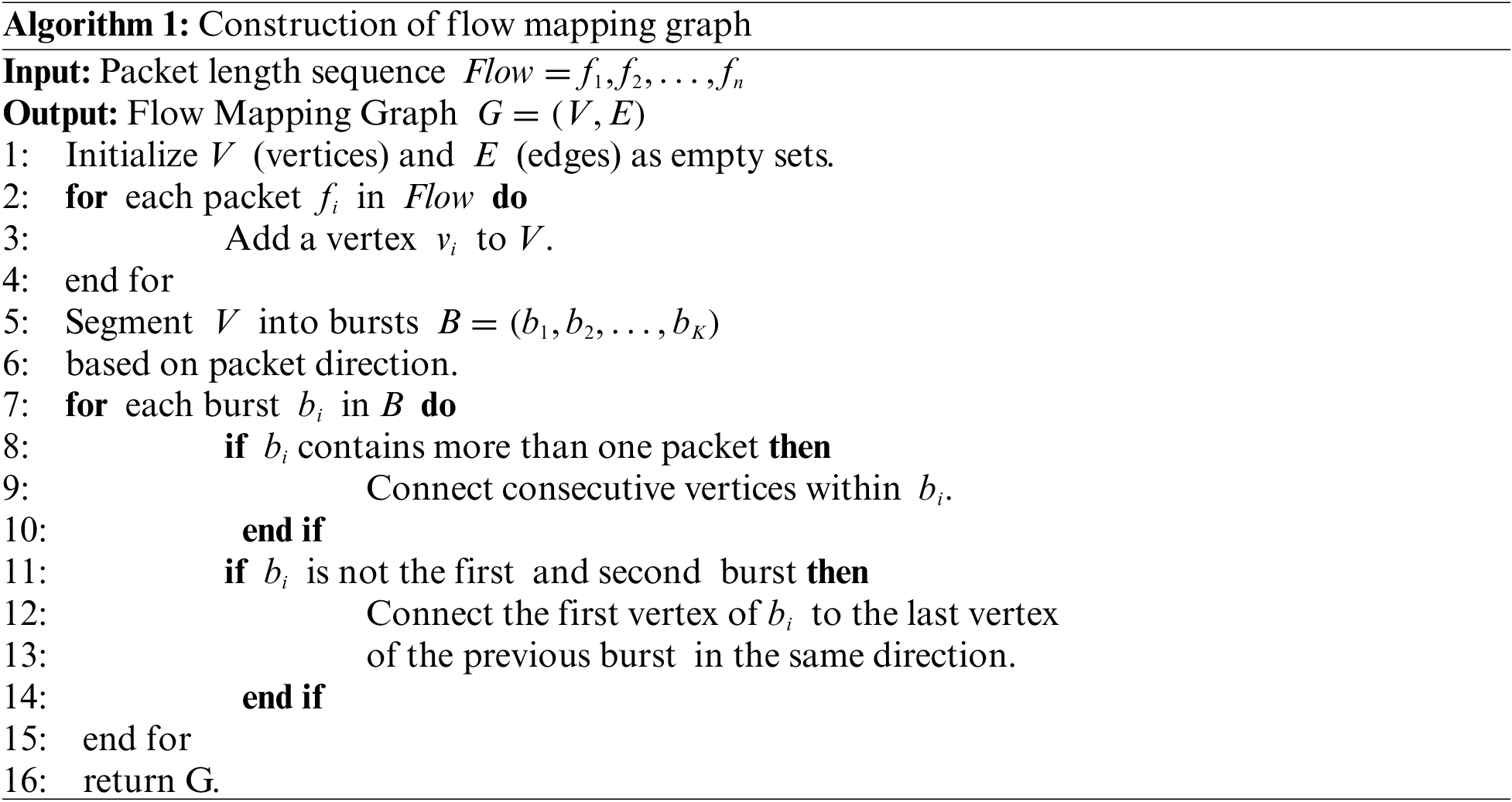
Algorithm 1 describes the FMG construction process. The algorithm uses a sequence of packet lengths for a specific flow as the input and outputs a traffic map G=(V,E). First, the vertex set V and edge set E are initialized, and then the vertex set is constructed using the packets as vertices (lines 1–4). Second, different bursts were obtained based on consecutive packets (lines 5–6). We then iterate each burst by checking whether the length of each burst is greater than 1, and if so, add sequential edges with timing characteristics (lines 7–10). Then, in bursts, jump-order edges are obtained by connecting the last vertex of a burst with the first vertex of the previous burst in the same direction (lines 11–14), and the FMG representation results in G of the traffic are returned. The following explains why FMG is designed as a graphical representation of encrypted traffic. In general, an FMG can extract the features of encrypted traffic from three aspects:

(1) Packet-direction information: The vertices in the FMG contain the direction of the data packet, which is represented by positive and negative values. Positive values indicate that the packet was sent from the client to the server, and negative values indicate that the packet was sent from the server to the client.

(2) Packet-length information: Packet-length sequences and their mathematical variants are commonly used as key features in encrypted traffic classification [20,31]. Vertices in FMG are associated with corresponding packet lengths and can be used naturally by classifiers.

(3) Data packet bursts, as shown in the same color in Fig. 2b, are directional and key distinguishing features of classifier learning owing to their variability across different applications or websites. Packets, whether in the same or different directions, are interconnected through sequential and jump-order edges, facilitating the feature aggregation of each vertex. This method enhances the analysis of client-side request–response sequences, helping to quickly pinpoint and assess the correlation between successive client requests and responses. From the server perspective, this aids in swiftly identifying specific response patterns. During the feature aggregation phase, this approach allows for a more detailed aggregation of neighboring vertex features, enabling the TMC-GCN model to perform classification tasks more effectively.

3.2 TMC-GCN

With FMG, the encrypted traffic classification problem becomes a graph classification problem. Thus, a GNN can automatically extract and distinguish features from a graph structure [32]. The GNN was used as the basis for the TMC-GCN model. This section presents the design details of the GNN-based TMC-GCN classifier.

3.2.1 Overview of TMC-GCN

In this study, a TMC-GCN was constructed using a combination of a GCN, MLP, and linear fully connected layers, as shown in Fig. 3. The TMC-GCN model is structured into three main stages: data transformation, feature-aggregation transformation, and classification. (1) Data Transformation: This stage includes network traffic preprocessing and data processing. First, the pcap file of the original encrypted traffic is converted to JSON format, and streams with the same quintuple are extracted. The FMG is then fed into the embedding layer, which converts the features of the vertices into fixed-dimensional embedding vectors. The embedding vector obtained by the embedding layer was used as the input for the GCN in the next stage. (2) Feature Aggregation Transformation: Vertex features and those of their neighboring vertices are aggregated at this stage using both sequential and jump-order edges. The architecture included two pairs of GCN and MLP layers. Each GCN layer was followed by an MLP layer that applied a nonlinear transformation to the GCN output. The output of the first MLP layer becomes the input for the second GCN layer, enhancing feature aggregation. (3) Classification Stage: The final stage employs a graph-pooling layer to consolidate the vertex features into a graph-level feature vector. A fully connected layer then uses this vector to perform classification predictions. This structure facilitates detailed feature analysis and improves classification accuracy in network traffic analysis.

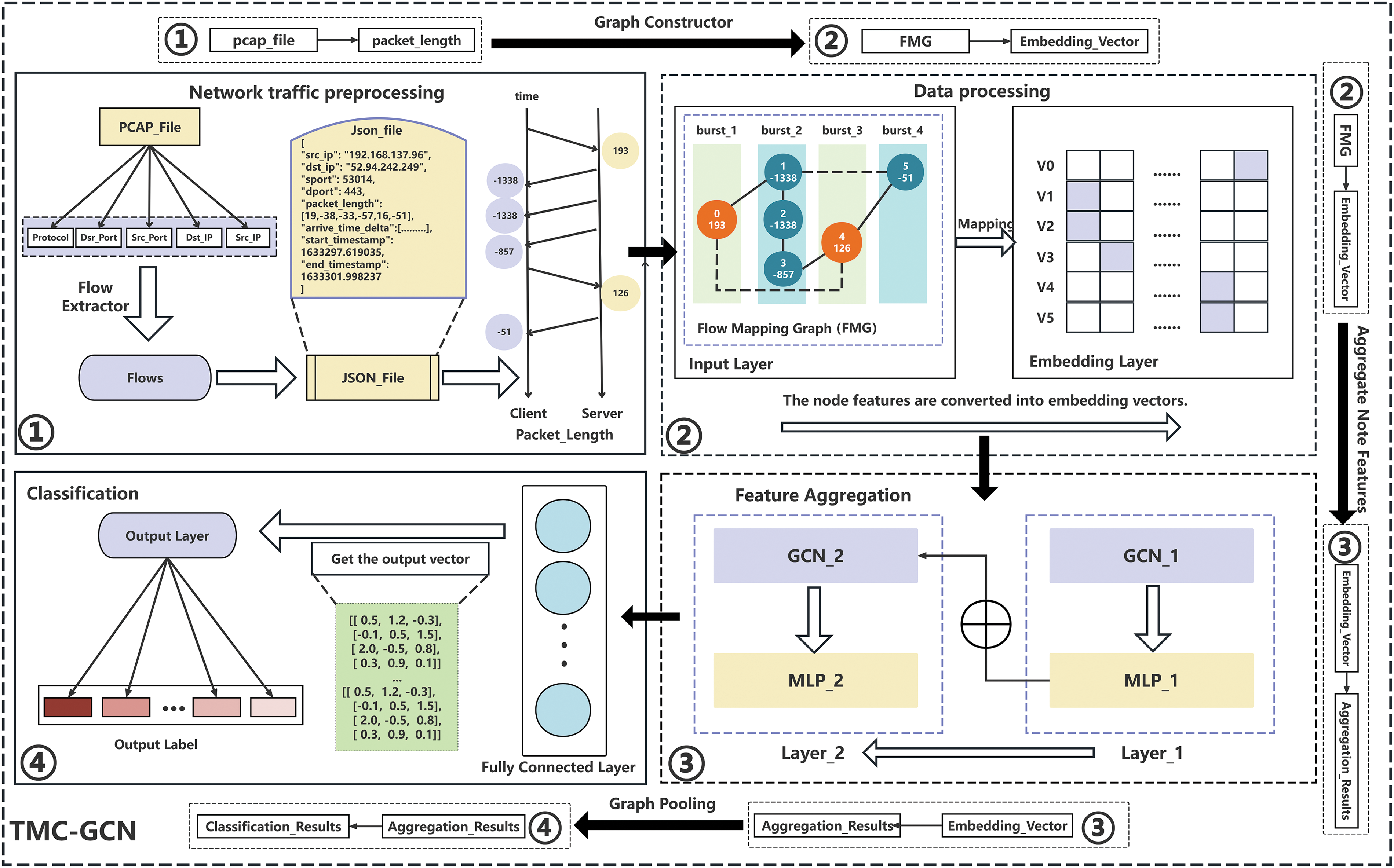
Figure 3: Model structure of TMC-GCN

3.2.2 Design Principle of Model Structure

a) Packet-direction information

The data transformation phase includes data preprocessing, construction of the FMG, and generation of embedding vectors. The details of the data transformation phase are described below.

Data preprocessing: First, the stream was extracted from the original pcap file according to the quintuples and converted into a JSON file. Second, the packet length sequence and positive and negative signs of each flow were recorded to indicate the direction. It is not necessary to determine which part of the packet is encrypted because this study mainly examines the impact of the network topology of the flow on the classification, and only the packet length and direction are used in the features, which can better protect the user’s privacy. Before constructing the FMG, we must perform the following.

(1) Data interception and dropping: Only the first 160 packets in the flow are used to control the amount of data and improve the efficiency. This measure aims to reduce computational burden and memory consumption. Simultaneously, to improve the quality of the dataset and reduce noise interference and abnormal flow, data packets that did not contain quintuples were discarded, considering that these may be caused by errors in data capture or recording processes. Flows with only one direction are discarded, as are flows with no more than three packets; thus, there is no case of no associated direction.

(2) Packet length correction: A packet with an absolute length greater than 1500 is split into multiple packets with a maximum length of 1500, and the original symbol is retained to normalize the data and simulate the actual network transmission limit. This step aims to avoid excessively large packets that interfere with the processing flow and to improve data utility.

(3) Vertex feature matrix creation: A zero matrix of the same length as the packet was created, and the length of the processed packet was assigned to this matrix. This matrix was added to the graph as a vertex feature. This provides each vertex in the graph with useful feature information for subsequent graph analysis.

Generating embedding vectors: The model uses an embedding layer to convert vertex features into vectors of fixed dimensions. The input to the embedding layer is the discrete feature index i, corresponding to the features of the vertices in the FMG, which is the packet length value with respect to the direction. This index is then mapped in the embedding matrix E into a continuous vector space of D dimensions, where E∈RN×D, N is the embedding dictionary’s size, embedding dictionary is represented as a mapping from the packet length to the embedding index, and D is the dimension of the embedding vector. We created an embedding dictionary, represented as a mapping from packet length to embedding index. The key is the length of the packet belt direction (−1500 bytes to 1500 bytes). When a specific packet length is received, this length can be used as the key to obtain the corresponding embedding vector index from the embedding dictionary. This vector was subsequently used as the input for the next layer. Embedding layers are introduced to map sparse data-length features to a more compact and continuous vector space for model learning and generalization, respectively. The floating-point representation of embedding vectors is more suitable for the optimization algorithms of neural networks. In addition, the embedding layer can effectively handle new length values that do not appear in the training data and generate embedded vectors for new features.

b) Feature aggregation transformation

This module is the core of the model, and it aggregates the characteristics of each vertex and its neighborhood vertices. By strengthening the connection between vertices using sequential and jump-order edges, the module can aggregate more comprehensive feature information. The module comprises two pairs of sequentially cascaded GCN and MLP. An MLP layer followed each GCN layer, and the MLP performed a nonlinear transformation of the GCN output. The input to the second layer of the GCN is the output of the first layer of the GCN after MLP processing. These two layers of the GCN and MLP together form a feature aggregation transformation layer, which then aggregates the feature vector output by the MLP through a graph pooling layer.

Vertex feature aggregation: Vertex feature aggregation is iterated using a two-layer GCN to balance complex structural information capture and computational efficiency (The two-layer GCN framework has been shown to strike an appropriate balance between performance and computational burden [33]). A GCN can comprehensively integrate the information of different vertices into the vertex features of an entire FMG. The high-dimensional feature representation of each vertex can be summarized through feature aggregation as a lower-latitude graph-level feature representation. Simultaneously, because of the design of sequential and jump-order edges in FMG, particularly jump-order edges, GCN can aggregate more comprehensive information than other graph structures. First, the initial vertex feature vector is derived from the embedding layer. The feature transformation of the initial vertex feature and feature aggregation of the neighborhood vertex is realized using Eq. (1), where hv(l) represents the hidden state of vertex v after the l-layer of the GCN, and σ is the activation function. N(v) is the set of neighboring vertices v, deg⁡(v) is the degree of vertex v, and W(l) is the first GCN weight matrix of the l layer.

hv(l+1)=σ(∑u∈N(v)∪{v}1deg⁡(u)deg⁡(v)W(l)hu(l))(1)

Nonlinear transformation: The model can be more flexible and extract higher-order and more complex features and relationships from the data through a nonlinear transformation. The TMC-GCN uses an MLP to perform a nonlinear transformation on the output of the GCN, which can map the input features to a higher level of abstract feature space, help the model better understand and process data, and improve its generalization ability. Nonlinear transformation is realized using Eq. (1), where hv(l) represents the output feature of vertex v in an L-layer GCN. Two linear transformation layers (W1(l) and W2(l)) and two offset items (b1(l) and b2(l)) introduce the ReLU activation function, and the ability for nonlinear transformation is added. MLP(⋅) stands for multi-layer perceptron, which is used to transform the output of GCN further, and h^v(l+1) is the feature of vertex v after MLP transformation. However, the combination of GCN and MLP can deal better with FMG graph data. This helps the model learn higher-level abstract feature representations of a graph. By fusing the graph structure information and nonlinear transformations, the model can better capture the complex relationships and characteristics of the data.

h^v(l+1)=MLP(hv(l))=σ(W2(l)ReLU(W1(l)hv(l)+b1(l))+b2(l))(2)

hG=∑v∈Vh^v(l)(3)

Graph-level feature aggregation: Post MLP, the data represent high-order abstract feature vectors obtained from multiple layers of nonlinear transformation and feature extraction. This vector is fed into a graph pooling layer, which aggregates vertex-level features into a graph-level representation by summing, capturing the overall structure and properties of the graph for the classification layer. Sum pooling (Eq. (3)) highlights important vertexes by weighting their features, thus preserving the differences in vertex features. Sum-pooling sums up all vertex features to form a comprehensive graph representation, which is suitable when vertex features are additive.

c) Classification

Mapping feature class: This step is key to classification and relies on fully connected layers to map graph-level features to the category space for classification. The input to the fully connected layer was the concatenation result of the graph-level features obtained from the operations of the graph convolution and pooling layers. These graph-level features are concatenated during forward propagation to obtain a vector, which is then linearly transformed by weight matrix multiplication and bias addition of Eq. (4). In the forward-propagation process, the input vector hG is multiplied by the weight matrix W, and the bias vector b is added to obtain the output vector y, which is a linear transformation from the input space to the output space. During training, the model updates the values of the weight matrix and bias vector using a backpropagation algorithm and gradient descent optimizer to minimize the loss function. Through continuous iterations and optimization, the model can learn an effective mapping from the input to the output.

y=Linear(hG)=WhG+b(4)

Loss function: The loss function used in this study is across-entropy loss function combined with weighting and label smoothing, as shown in Eq. (5). Where N is the number of samples in the batch, yi is the true label of sample i, and y^i is a one-hot-encoded vector with only one element of 1 (representing the class of the input sample) and the rest of the elements of 0 and is the predicted probability of the ith sample. ϵ denotes the label smoothing parameter, and K is the number of categories. Label smoothing enhances the model’s prediction by distributing some probability from the correct class to other classes, thereby reducing the risk of overfitting. Cross-entropy loss measures the difference between the predicted probability and the true label; a smaller loss value indicates a more accurate model prediction. The generalization ability and stability of the model can be effectively improved by combining label smoothing and cross-entropy loss.

Loss=−∑i=1N[(1−ϵ)⋅yi+ϵK]log⁡y^i(5)

4  Experimental Evaluation

In this part, we evaluate the effectiveness of FMG and TMC-GCN modes. This paper compared the performance of TMC-GCN and other encrypted traffic classification models, tested the effectiveness of FMG, adjusted the parameters of the model, and finally designed an ablation experiment.

4.1 Experimental Setup

This study compares the performance of other encrypted traffic classification models and tests the performance of TMC-GCN on the CICIOT2023, CICAAGM2017, and ISCXVPN2016 datasets. To verify the interpretability of FMG and the performance and versatility of TMC-GCN, experiments are carried out on the GraphDapp dataset. The 38 application categories of this dataset were selected, and 20 flows were randomly selected from each category, resulting in a total of 760 flows. The effectiveness of FMG is measured by calculating the pairwise distance and graph edit distance of the TMC-GCN model are adjusted. Finally, an ablation experiment is carried out to determine whether the jump-order edge and packet length provide additional valuable information.

The comparison model used in this paper is as follows:

(1) CNN+D [34]: uses packet direction information to build a CNN to classify encrypted traffic from different websites.

(2) AppScanner [35]: uses bidirectional streaming features (i.e., outgoing and incoming) to extract features about packet length and interval time from the stream.

(3) MIMITIC [21]: is a multi-modal approach that lever-ages deep learning, using CNN and GRU to learn the first 576 bytes of payload and message protocol fields, respectively.

(4) FS-Net [19]: takes packet length sequence as input, uses bidirectional GRU for feature encoding, and introduces a reconstruction mechanism in Auto Encoder to ensure the validity of the learned features.

(5) App-Net [23]: uses LSTM and CNN to learn the packet length and payload byte sequence of the initial packet, respectively.

(6) GraphDapp [12]: uses the graph structure of the TIG as the information representation for encrypted Distributed Application (DApp) flows, implicitly preserving many of the characteristics of bidirectional client-server interactions. Dapp finger-printing is transformed into a graph classification problem, with an MLP and a fully connected layer used to construct the GraphDapp model.

(7) FB-GNN [29]: proposes a graph construction method that directly creates edges based on the temporal relationships of packets in a stream and leverages a geometric learning model to learn vertex, edge, and global features.

In this study, the True Positive Rate (TPR), False Positive Rate (FPR), precision, recall, and F1 value were used as criteria to test the performance of the TMC-GCN. These criteria are computed as shown in Eqs. (6)–(10):

TPR=TPTP+FN=Recall(6)

FPR=FPFP+TN(7)

Precision=TPTP+FP(8)

Accuracy=TP+TNTP+FP+FN+TN(9)

F1=2×Precison×RecallPrecision+Recall(10)

4.2 Dataset Description

The CICIOT2023, ISCXVPN2016, CICAAGM2017, and GraphDapp datasets were used for the testing. The total data volume was 130 gigabytes, with more than one million streams.

(1) CICIOT2023 Dataset: This large-scale attack dataset in a real-time Internet environment is derived from 33 attacks classified into seven categories: DDoS, DoS, reconnaissance, web-based, brute force, spoofing, and Mirai. These attacks are performed against malicious Internet devices on other Internet devices. These include ACK fragmentation, UDP flood, SlowLoris, ICMP flood, RSTFIN flood, PSHACK flood, HTTP flood, UDP fragmentation, and TCP-based attacks. It contains 33 attacks, such as flood, SYN flood, SynonymousIP flood, Dictionary brute force, Arp spoofing, Ping sweep, Sql injection, and UDPPlain.

(2) ISCXVPN2016 Dataset: This dataset was designed for network traffic analysis and covers 14 different traffic types captured through regular and VPN sessions, such as VOIP, VPN-voip, and P2P. By simulating the network activities of users Alice and Bob, this dataset generates data using a variety of applications and services (such as Skype, Facebook, and YouTube), which ensures its practical application value and wide applicability. The dataset pays special attention to the distinction between VPN-encrypted traffic and unencrypted traffic, uses tools such as Wireshark and tcpdump for high-quality data capture, and shuts down all non-target applications during the capture process to ensure data purity. This makes the ISCXVPN2016 dataset not only important for the development of intrusion detection systems and traffic management optimization in the field of network security but also provides an experimental platform for academic research on network traffic analysis and data mining.

(3) CICAAGM2017 Dataset: This dataset was created to address the challenge posed by advanced Android malware, which can detect emulators used by analysts and alter its behavior to evade detection. To overcome this problem, researchers have installed applications on real Android devices to capture network traffic. The dataset included 1900 apps divided into three categories: 250 adware apps, including Airpush, Dowgin, Kemoge, Mobidash, and Shuanet, which not only display ads but may also steal user information or takeover the device; 150 generic malware applications, such as AV-pass, FakeAV, FakeFlash/FakePlayer, GGtracker, and Penetho, which perform information theft, fraud, or other malicious activities by masquerading as commonly used applications or services, and 1500 good applications.

(4) GraphDapp Dataset: The GraphDApp dataset was selected by deploying the Wireshark tool on campus laboratory routers at various universities in China. It focuses on monitoring the network traffic generated when users access the top 40 most popular Ethereum distributed applications (DApps) using a Chrome browser. Each DApp in the dataset has a corresponding network traffic record, detailing the number of traffic packets per DApp, such as Joyso (395 traffic), Bancor (290 traffic), and Idex (3119 traffic). For Development tool classes: Oxdrop (5016 traffic), Golem (2207 traffic), Financial services UQUID (7290 traffic), Aave Protocol (4004 traffic). The dataset contains information such as access time, source and destination IP addresses, port number, protocol used, packet length, and TCP/IP flag, but does not include encrypted payload content to protect user privacy and data security.

4.3 Result

This subsection explores the interpretability of FMG and the performance of the TMC-GCN mode. First, the stream and graph edit distances were used to test the interpretability of the FMG. Next, the performances of TMC-GCN and other classifiers were evaluated. Finally, parameter adjustment and ablation experiments are performed on the proposed model.

4.3.1 FMG Test Results

In this study, the flow distance and Graph Edit Distance (GED) [36], based on packet length sequences were used to measure the similarity in FMG, with smaller distances indicating greater similarity. For each of the 38 application categories, 20 streams were randomly selected for each category for pairwise distance calculation. Because of the high computational load of the GED, only five flows per category were selected for these calculations. The results are displayed in Fig. 4a and 4b. In each figure, the dots (blue in Fig. 4a and red in 4b) indicate the average intraclass distance within the same application, whereas the boxplots illustrate the typical interclass distances with other applications. By comparing Fig. 4a and 4b, the following conclusions can be drawn:

(1) In the box plot of the flow distance with length sequences, there were no cases in which the intraclass distance was smaller than the minimum interclass distance. This implies that when using a flow distance with a length sequence, the discrimination between the intra-class and interclass distances is not obvious, and it is difficult to effectively distinguish flows in the same application from flows in different applications. Almost all intraclass distances of the FMG graph edit distances were smaller than the minimum interclass distances. This shows that when using the graph edit distance, the discrimination between the intraclass and interclass distances is very clear and flows in the same application can be effectively distinguished from those in different applications.

(2) For the flow distance using the length sequences, all intraclass distances exceeded the median of the interclass distances (blue line in Fig. 4a). Conversely, in the FMG graph edit distance, all intraclass distances were below the median of the interclass distances (red line in Fig. 4b). This suggests that the flow distance with length sequences exhibits considerable uncertainty and instability when dealing with flows from different applications, with a lack of a clear distinction between intraclass and interclass distances, leading to limited robustness and reliability of the similarity measure. By contrast, FMG’s graph edit distance demonstrates clear discrimination between different application flows, with a pronounced difference between intraclass and interclass distances, confirming its robustness and reliability as a similarity measure.

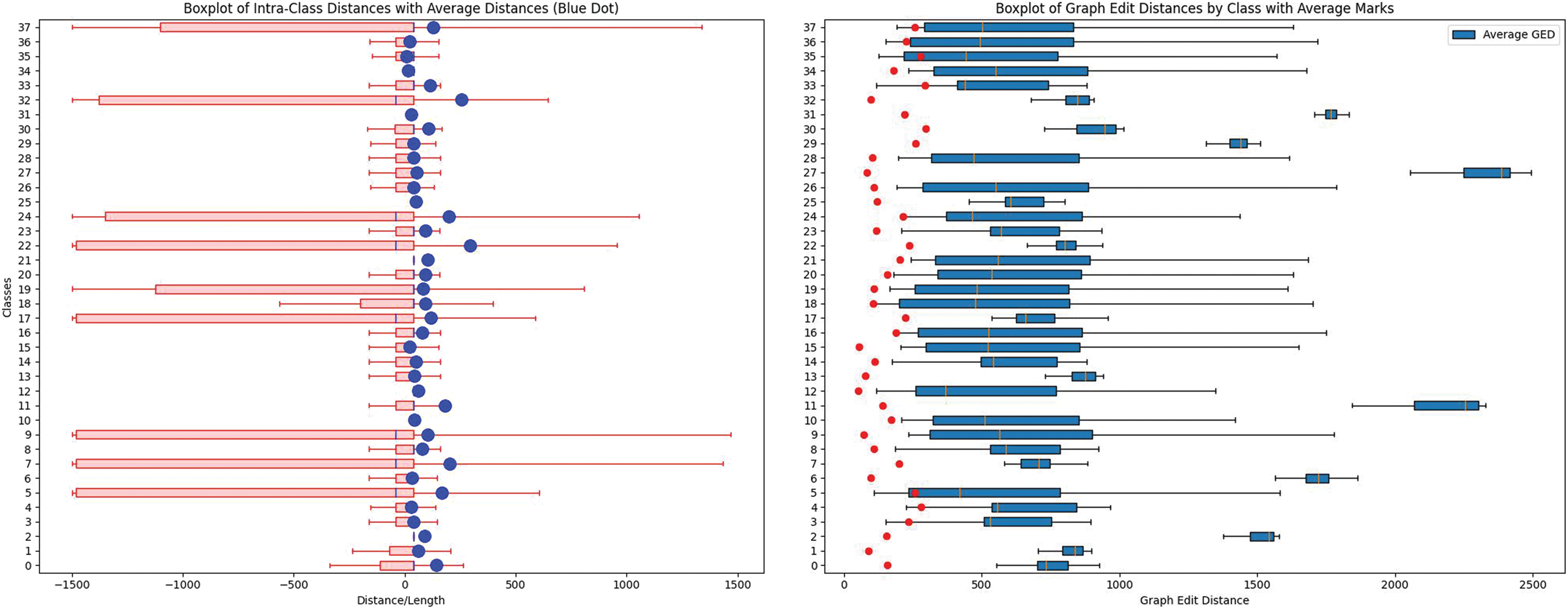
Figure 4: Boxplots of distances in data sequences and graphs (The left picture is (a) Boxplot of flow distance with packet-length sequences; The right picture is (b) Boxplot of GED for FMG)

4.3.2 Performance Test Results of TMC-GCN

(1) The TMC-GCN model demonstrated superior performance compared with the other models on the CICIOT2023, ISCXVPN2016, CICAAGM2017, and GraphDapp datasets, as shown in Table 2. In particular, on the CICIOT2023 and GraphDapp datasets, TMC-GCN significantly outperformed the competitors. Although it trails App-Net by a few percentage points on the ISCXVPN2016 dataset, the difference is minimal. Overall, TMC-GCN led by several percentage points across various metrics, highlighting its robust capability to handle complex datasets by effectively capturing intricate relationships and structural data.

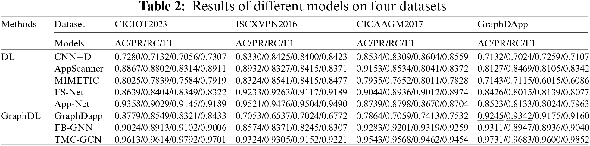
(2) Table 2 shows that the TMC-GCN model excels across four datasets—CICIOT2023, ISCXVPN2016, CICAAGM2017, and GraphDapp—in key performance metrics such as accuracy (AC), precision (PR), recall (RC), and F1 score (F1). Whereas other models may perform well on specific datasets, TMC-GCN exhibits greater stability in different tasks. For example, although GraphDapp and FB-GNN exhibit strong results on their respective datasets, they fall short of the others, underscoring the superior capability of TMC-GCN in handling complex datasets and cross-domain applications. This highlights TMC-GCN as a versatile classifier and demonstrates the effectiveness of jump-order edges in FMG.

(3) Drawing inspiration from the GraphDapp model cited in the literature [12] and enhancing it by adding jump-order edges, the TMC-GCN model was redesigned to improve performance. As depicted in Figs. 5 and 6, TMC-GCN exhibited superior performance on the GraphDapp dataset across 38 randomly selected categories. The model consistently achieved a TPR above 0.94, indicating high accuracy in identifying positive examples, and maintained an FPR below 0.004, highlighting its precision. Accuracy rates generally exceed 0.95, confirming the reliability of the model. In addition, the recall and F1 scores were strong, demonstrating the effective coverage of positive samples by TMC-GCN and its ability to balance precision and recall. These findings highlighted the stability and high recognition accuracy of the TMC-GCN model.

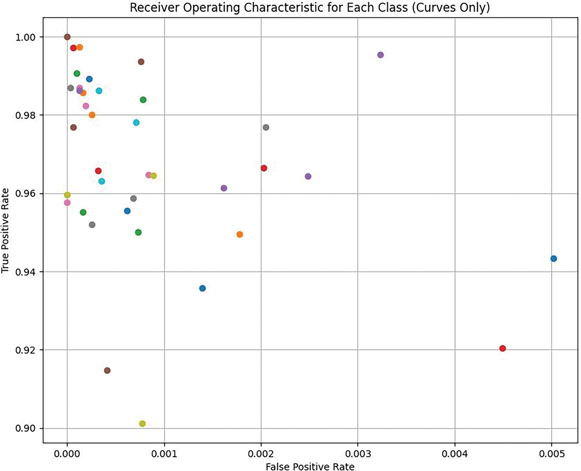
Figure 5: TPR and FPR test results for different categories

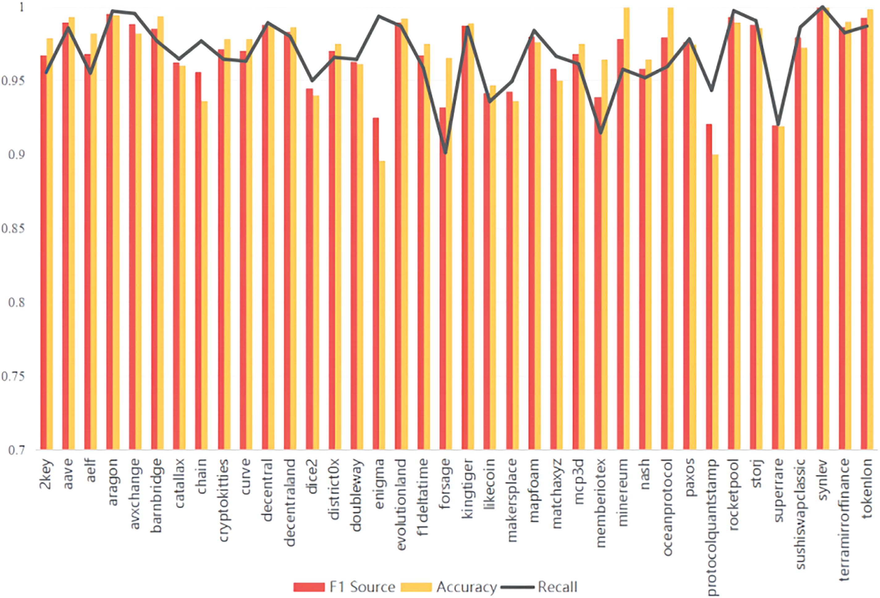
Figure 6: Precision, F1 score, and recall for 38 random app categories in the GraphDapp dataset

4.3.3 Hyperparameter Selection

In this section, the conventional and key parameters used by the TMC-GCN are introduced, and their influence on the trade-off between the classification performance and training speed in each epoch is studied. Because the data in different datasets affected the judgment of the hyperparameters, the GraphDapp dataset was used for the experiment.

(1) General parameters: Table 3 lists the test accuracy and training loss for various batch sizes. The training speed (TS) significantly increased with larger batch sizes; for example, a batch size of 2 required 302 s/epoch, whereas a size of 64 required only 24 s/epoch, indicating the efficient use of computational resources and faster training. The highest test accuracy of 0.9784 was achieved with a batch size of 64, indicating optimal learning at this size. Table 4 shows the test accuracy for different learning rates with significant variations. Extremely low (10−6) or high (5×10−3) learning rates lead to slow convergence or oscillation during training, respectively, hindering optimal solution attainment. However, a learning rate of 5×10−4 yielded the highest test accuracy of 0.9885, indicating stable convergence to the optimal solution. Fig. 7 shows that after 25 epochs, the changes in training loss and accuracy were minimal, making further training less beneficial. Therefore, 25 epochs was a good balance, ensuring good model performance while saving time and computational resources.

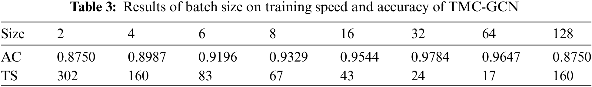
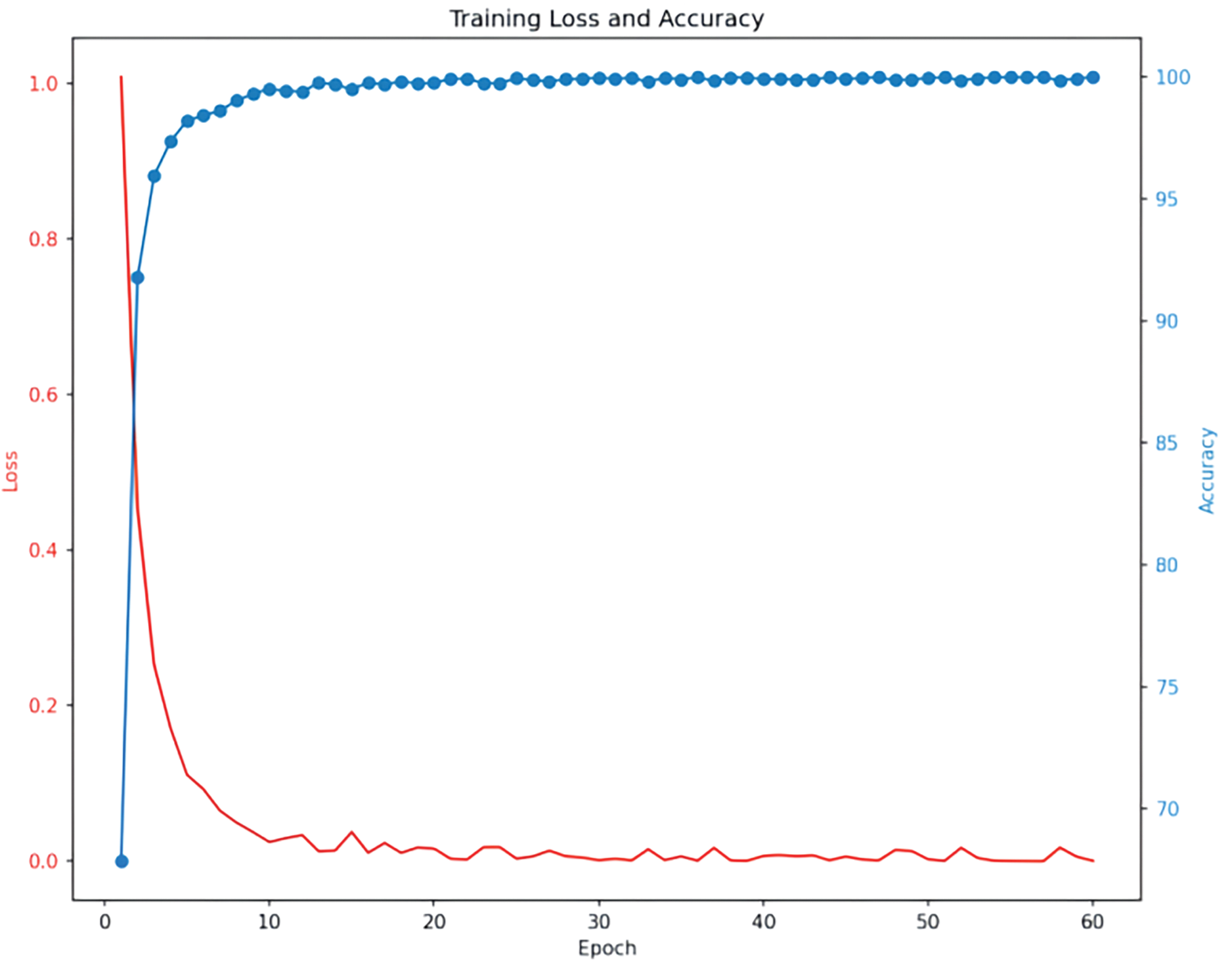
Figure 7: Effect of epochs on training loss and test accuracy

(2) Key parameters: The success of this study hinged on the construction of the FMG, with the number and length of packets being crucial factors. Insufficient packets result in fewer diverse FMGs per flow, hindering classification. Conversely, an FMG built with too many or too long packets becomes overly complex, increasing time costs and diminishing model performance. The effects of packet number and maximum packet length on the TMC-GCN are detailed below.

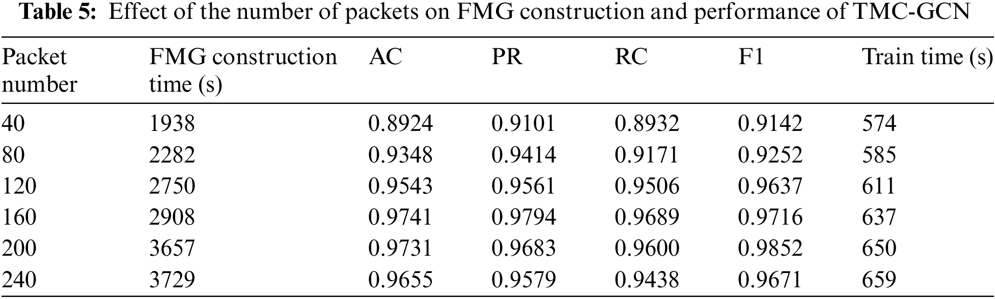
Maximum number of packets: We analyzed 171,403 streams from 19 classes in the GraphDapp dataset. As listed in Table 5, the performance of the models (AC, PR, RC, and F1) improved as the Packet Number increased, peaking at 160 packets. Beyond this, performance metrics such as AC, PR, RC, and F1 began to decline, as exemplified by the lower scores at 240 packets than at 160 packets. Despite the increased construction and training times for FMG with higher packet numbers, they were still within acceptable limits. This suggests that a Packet Number of 160 optimally balances performance and computational efficiency, effectively capturing the necessary flow information for optimal classification without overcomplicating the model.

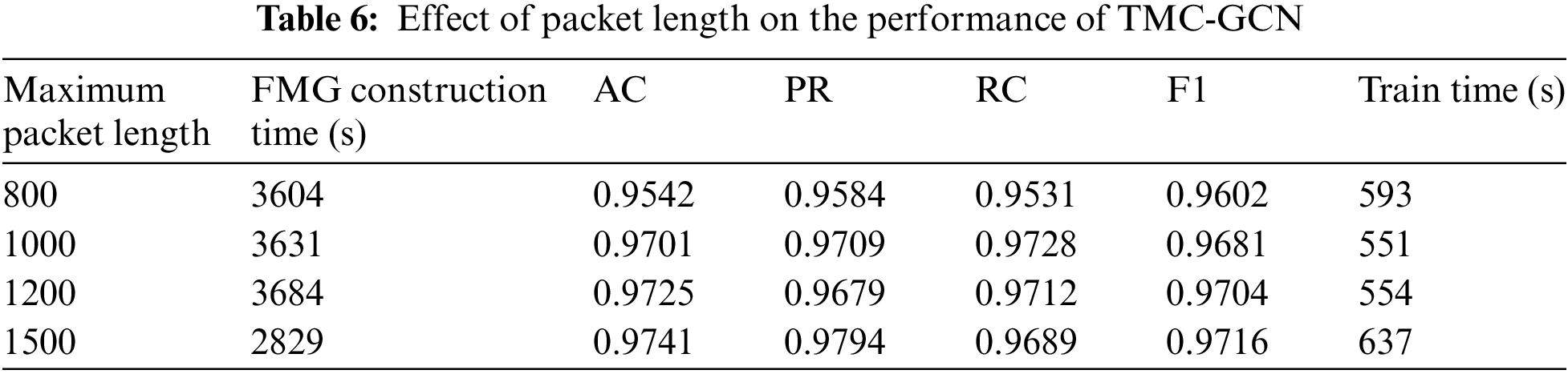
Maximum packet length: Before constructing an FMG, packet lengths must be corrected. If a packet length exceeds the maximum allowed, it is split into multiple packets, retaining the original symbol for normalization. As shown in Table 6, the FMG construction time initially increases with packet length but then decreases because fewer packets need to be split. At a packet length of 1500 B, the model performance indicators (AC, PR, RC, and F1) reached their highest values. Although the construction and training times increased slightly, they remained within acceptable limits. This indicates that a packet length of 1500 B strikes an optimal balance between information content and redundancy, reducing the packet splitting complexity and enhancing the construction and training efficiency, resulting in the best classification performance.

4.3.4 Ablation Experiment

In this subsection, the baseline model TMC-GCN is tested through ablation experiments, and the influence of the original features of the vertices and jump-order edges in FMG on the model is tested by having jump-order edges and changing the original features of the vertices (packet length).

(1) Effect of jump-order edges in FMG on the model

This part analyzes the importance of jump-order edges in FMG, selects 19 types of traffic, a total of 34,304 flows for testing, and compares the trained TMC-GCN model as the baseline model with the “FMG” model without adding jump-order edges as the input, called Model_1 here. The results are shown in the confusion matrix in Fig. 8, where TMC-GCN is significantly different from Model_1 in terms of classification performance. TMC-GCN outperforms Model_1 in multiple categories, as the higher diagonal elements of the confusion matrix indicate the number of correct classifications. For example, the number of correct classifications of class 0 for TMC-GCN was 1805, while that for Model_1 was only 760. Similarly, TMC-GCN had 9676 correct classifications in Class 4, whereas Model_1 had 8405 correct classifications. In addition, the correct classification number of TMC-GCN was significantly higher than that of Model 1 for multiple categories, such as categories 8, 14, and 18.

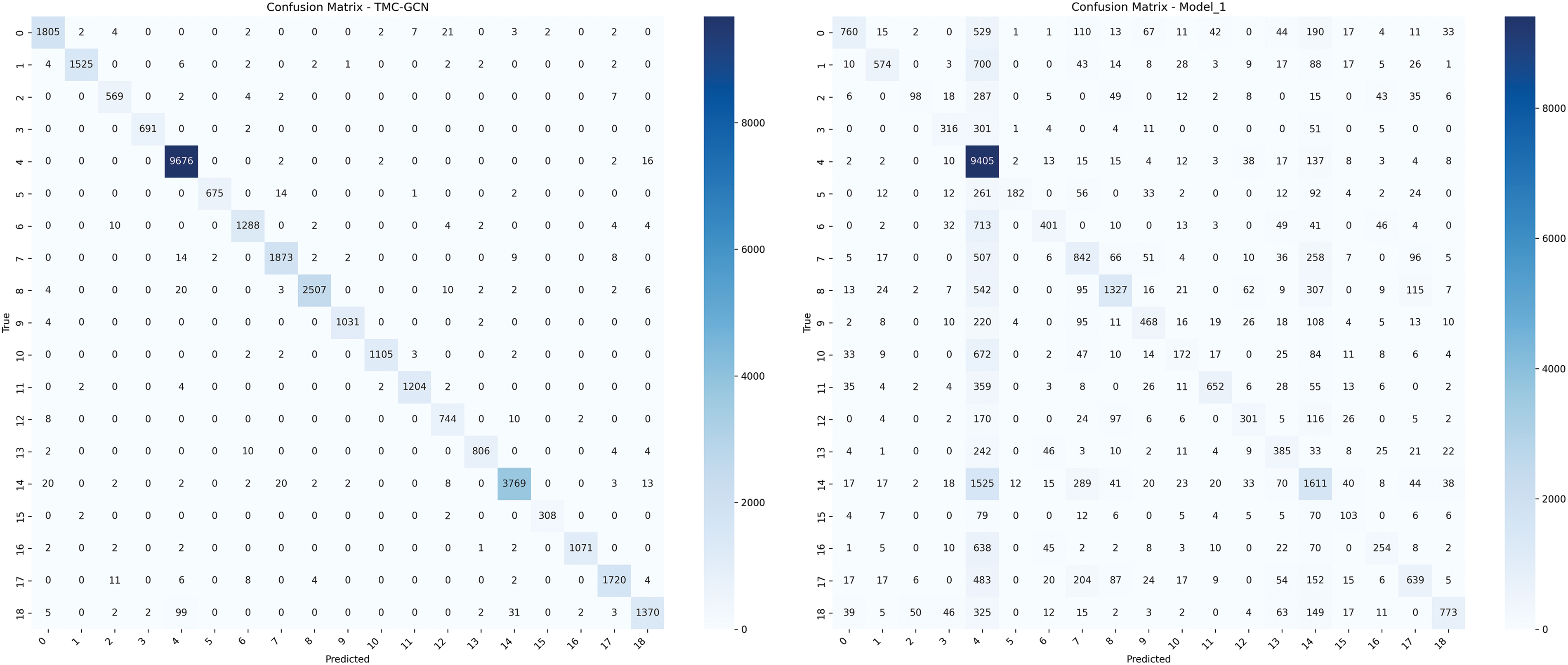
Figure 8: Performance comparison between the baseline model and the jump-order edge free model

This shows that the introduction of reordering edges significantly improves the classification performance of the model, particularly for complex categories and categories with a large number of samples. By capturing the relationship between distant vertices (packets in the same direction) in the graph structure, the jump-order edge enhances the model’s ability to perceive global information, thereby improving the classification accuracy. In contrast, Model_1 relies only on local neighborhood information, which cannot effectively capture the relationship between distant vertices, leading to a decrease in classification performance. The excellent performance of the TMC-GCN shows that the jump-order edges in the FMG play a key role in the model, which can significantly improve its global information capture ability and classification accuracy.

(2) The influence of the original characteristics of vertexes (packet length with direction) on the model in FMG

In this part, the original feature of the vertex, namely, the packet length with direction, is replaced by the zero matrix during input. At this time, the “FMG” only has the topology of the traffic, but does not have the original feature. These data were used as the input for the model training, defined as Model_2. The results are shown in Fig. 9, and a comparison of the two confusion matrices indicates that TMC-GCN (left panel) performs significantly better than Model_2 without the packet length feature (right panel) on multiple categories. For example, the number of correct classifications in class 0 was 1805 for TMC-GCN, whereas that in Model_2 was 207. Similarly, TMC-GCN had 3769 correct classifications in class 14, whereas Model_2 had only 1744.

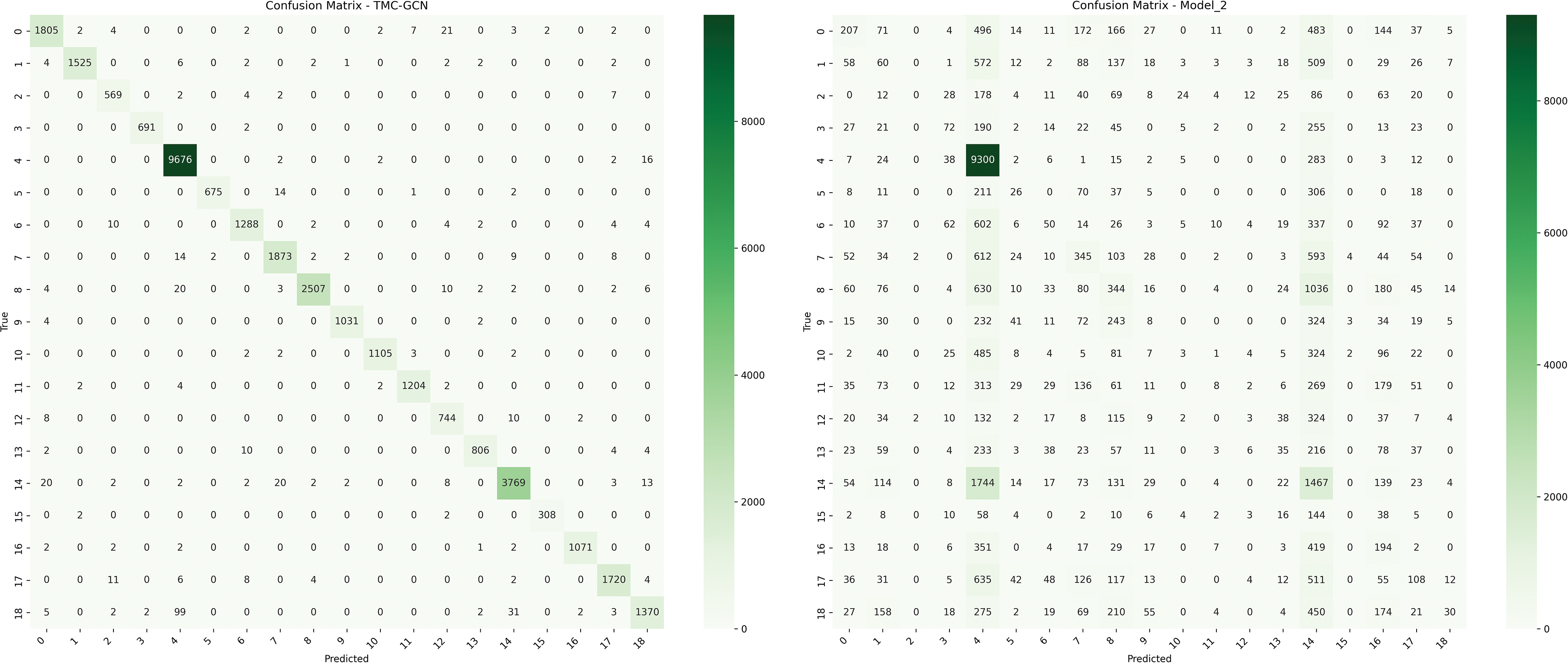
Figure 9: Performance comparison between the baseline model and the vertex-free original feature (packet length) model

The introduction of the packet length feature as a vertex feature significantly improved the classification performance of the model. This is because the packet length feature can provide important information about the network traffic and help the model better distinguish between different classes of traffic patterns. Specifically, packet length characteristics can capture the characteristics of different types of traffic when transmitting data; for example, some specific applications or protocols may produce packets of a specific length. By introducing these features, the model can identify and classify different types of traffic more accurately, thereby improving the overall classification accuracy. The excellent performance of TMC-GCN shows that the packet length feature plays an important role in the network traffic classification task, which can significantly improve the classification ability and accuracy of the model.

5  Conclusion

In this study, we explored the problem of encrypted traffic classification based on neural networks by fusing GNN variants of the GCN and MLP. FMG and TMC-GCN models for the FMG setting were proposed, and the encrypted traffic identification task was transformed into a graph classification problem suitable for multiple data sources and application scenarios. Tests on multidomain datasets, such as CICIOT2023, ISCXVPN2016, CICAAGM2017, and GraphDapp, show that the performance of the TMC-GCN model using FMG as the network traffic topology structure graph is not only superior to other models but also stable and efficient on different domains and datasets. However, although the construction cost of FMG and the computational cost of TMC-GCN are within the acceptable range, there is still room for improvement. In the future work, firstly, we will further optimize the construction algorithm of FMG from the perspective of time complexity and space complexity. Secondly, we will design a more suitable model for FMG to further reduce the computational cost of TMC-GCN. Finally, we will test the performance of our model against state-of-the-art deep learning methods on large-scale network data.

Acknowledgement: The authors would like to thank the support and help from the School of Cyberspace Security of Zhengzhou University, the PLA Information Engineering University and the Key Laboratory of Network Cryptography Technology of Henan Province. Thanks to the National Key Research and Development Program project for the financial support of this paper.

Funding Statement: This work was supported by the National Key Research and Development Program of China No. 2023YFA1009500.

Author Contributions: The authors confirm contribution to the paper as follows: conceptualization, methodology, Baoquan Liu; formal analysis, investigation, Baoquan Liu, Xi Chen, Qingjun Yuan and Degang Li; writing—original draft preparation, Baoquan Liu; writing—review and editing, Baoquan Liu, Xi Chen, Qingjun Yuan, Degang Li and Chunxiang Gu; supervision, resources, funding acquisition, Chunxiang Gu. All authors reviewed the results and approved the final version of the manuscript.

Availability of Data and Materials: The data that support the findings of this study are available from the submitted author, Baoquan Liu, upon reasonable request.

Ethics Approval: Not applicable.

Conflicts of Interest: The authors declare no conflicts of interest to report regarding the present study.

References

1. S. Rezaei and X. Liu, “Deep learning for encrypted traffic classification: An overview,” IEEE Commun. Mag., vol. 57, no. 5, pp. 76–81, 2019. doi: 10.1109/MCOM.2019.1800819. [Google Scholar] [CrossRef]

2. R. Sharma, S. Dangi, and P. Mishra, “A comprehensive review on encryption based open source cyber security tools,” in 2021 6th Int. Conf. Signal Process., Comput. Cont. (ISPCC), 2021, pp. 614–619. doi: 10.1109/ISPCC53510.2021.9609369. [Google Scholar] [CrossRef]

3. R. Vinayakumar, K. P. Soman, and P. Poornachandran, “Applying convolutional neural network for network intrusion detection,” in 2017 Int. Conf. Adv. Computi., Communi. Inform. (ICACCI), 2017, pp. 1222–1228. doi: 10.1109/ICACCI.2017.8126009. [Google Scholar] [CrossRef]

4. S. A. Althubiti, E. M. Jones, and K. Roy, “LSTM for anomaly-based network intrusion detection,” in 2018 28th Int. Telecommun. Netw. Appli. Conf. (ITNAC), 2018, pp. 1–3. doi: 10.1109/ATNAC.2018.8615300. [Google Scholar] [CrossRef]

5. S. H. Park, H. J. Park, and Y. J. Choi, “RNN-based prediction for network intrusion detection,” in 2020 Int. Conf. Artif. Intell. Inform. Commun. (ICAIIC), 2020, pp. 572–574. doi: 10.1109/ICAIIC48513.2020.9065249. [Google Scholar] [CrossRef]

6. P. Wang, X. Chen, F. Ye, and Z. Sun, “A survey of techniques for mobile service encrypted traffic classification using deep learning,” IEEE Access, vol. 7, pp. 54024–54033, 2019. doi: 10.1109/ACCESS.2019.2912896. [Google Scholar] [CrossRef]

7. G. Aceto, D. Ciuonzo, A. Montieri, and A. Pescap’e, “DISTILLER: Encrypted traffic classification via multimodal multitask deep learning,” J. Netw. Comput. Appl., vol. 183–184, 2021, Art. no. 102985. doi: 10.1016/j.jnca.2021.102985. [Google Scholar] [CrossRef]

8. J. Lan, X. Liu, B. Li, Y. Li, and T. Geng, “DarknetSec: A novel self-attentive deep learning method for darknet traffic classification and application identification,” Comput. Secur., vol. 116, 2022, Art. no. 102663. doi: 10.1016/j.cose.2022.102663. [Google Scholar] [CrossRef]

9. L. Zhang, L. Tan, H. Shi, H. Sun, and W. Zhang, “Malicious traffic classification for IoT based on graph attention network and long short-term memory network,” in 2023 24st Asia-Pacific Netw. Operat. Manag. Symp. (APNOMS), 2023, pp. 54–59. [Google Scholar]

10. F. Scarselli, M. Gori, A. C. Tsoi, M. Hagenbuchner, and G. Monfardini, “The graph neural network model,” IEEE Trans. Neural Netw., vol. 20, no. 1, pp. 61–80, 2009. doi: 10.1109/TNN.2008.2005605. [Google Scholar] [PubMed] [CrossRef]

11. J. Bruna, W. Zaremba, A. Szlam, and Y. LeCun, “Spectral networks and locally connected networks on graphs,” 2014, arXiv:1312.6203. [Google Scholar]

12. M. Shen, J. Zhang, L. Zhu, K. Xu, and X. Du, “Accurate decentralized application identification via encrypted traffic analysis using graph neural networks,” IEEE Trans. Inf. Forensics Secur., vol. 16, pp. 2367–2380, 2021. doi: 10.1109/TIFS.2021.3050608. [Google Scholar] [CrossRef]

13. K. Al-Naami et al., “Adaptive encrypted traffic fingerprinting with bi-directional dependence,” in Proc. 32nd Annual Conf. Comput. Secur. Appl. ACSAC ’16, New York, NY, USA, Association for Computing Machinery, 2016, pp. 177–188. doi: 10.1145/2991079.2991123. [Google Scholar] [CrossRef]

14. M. Jiang et al., “Accurate mobile-app fingerprinting using flow-level relationship with graph neural networks,” Comput. Netw., vol. 217, 2022, Art. no. 109309. doi: 10.1016/j.comnet.2022.109309. [Google Scholar] [CrossRef]

15. A. H. Lashkari, A. F. A. Kadir, H. Gonzalez, K. F. Mbah, and A. A. Ghorbani, “Towards a network-based framework for android malware detection and characterization,” in 2017 15th Annual Conf. Priv., Secur. Trust (PST), 2017, pp. 233–23309. doi: 10.1109/PST.2017.00035. [Google Scholar] [CrossRef]

16. E. C. P. Neto, S. Dadkhah, R. Ferreira, A. Zohourian, R. Lu and A. A. Ghorbani, “CICIoT2023: A real-time dataset and benchmark for large-scale attacks in iot environment,” Sensors, vol. 23, no. 13, 2023, Art. no. 5941. doi: 10.3390/s23135941. [Google Scholar] [PubMed] [CrossRef]

17. G. Draper-Gil, A. H. Lashkari, M. S. I. Mamun, and A. A. Ghorbani, “Characterization of encrypted and VPN traffic using time-related features,” in Int. Conf. Inform. Syst. Secur. Priv., Rome, Italy, 2016, vol. 1, 2016, 407–414. [Google Scholar]

18. X. Han et al., “DE-GNN: Dual embedding with graph neural network for fine-grained encrypted traffic classification,” Comput. Netw., vol. 245, 2024, Art. no. 110372. doi: 10.1016/j.comnet.2024.110372. [Google Scholar] [CrossRef]

19. C. Liu, L. He, G. Xiong, Z. Cao, and Z. Li, “FS-Net: A flow sequence network for encrypted traffic classification,” in IEEE INFOCOM 2019-IEEE Conf. Comput. Commun., 2019, pp. 1171–1179. doi: 10.1109/INFOCOM.2019.8737507. [Google Scholar] [CrossRef]

20. T. Van Ede et al., “FlowPrint: Semi-supervised mobile-app fingerprinting on encrypted network traffic,” in Netw. Distrib. Syst. Secur. Symp. (NDSS), San Diego, CA, USA, 2020. doi: 10.14722/ndss.2020.24412. [Google Scholar] [CrossRef]

21. G. Aceto, D. Ciuonzo, A. Montieri, and A. Pescapè, “MIMETIC: Mobile encrypted traffic classification using multimodal deep learning,” Comput. Netw., vol. 165, 2019, Art. no. 106944. doi: 10.1016/j.comnet.2019.106944. [Google Scholar] [CrossRef]

22. T. Shapira and Y. Shavitt, “FlowPic: A generic representation for encrypted traffic classification and applications identification,” IEEE Trans. Netw. Serv. Manag., vol. 18, no. 2, pp. 1218–1232, 2021, 2021. doi: 10.1109/TNSM.2021.3071441. [Google Scholar] [CrossRef]

23. X. Wang, S. Chen, and J. Su, “App-Net: A hybrid neural network for encrypted mobile traffic classification,” in IEEE INFOCOM 2020-IEEE Conf. Comput. Commun. Workshops (INFOCOM WKSHPS), 2020, pp. 424–429. doi: 10.1109/INFOCOMWKSHPS50562.2020.9162891. [Google Scholar] [CrossRef]

24. X. Liu et al., “Attention-based bidirectional gru networks for efficient https traffic classification,” Inf. Sci., vol. 541, no. 2, pp. 297–315, 2020. doi: 10.1016/j.ins.2020.05.035. [Google Scholar] [CrossRef]

25. X. Lin, G. Xiong, G. Gou, Z. Li, J. Shi and J. Yu, “ET-BERT: A contextualized datagram representation with pre-training transformers for encrypted traffic classification,” in Proc. ACM Web Conf. 2022, WWW ’22, Lyon, France, Association for Computing Machinery, 2022, pp. 633–642. doi: 10.1145/3485447.3512217. [Google Scholar] [CrossRef]

26. M. Lotfollahi, R. S. H. Zade, M. J. Siavoshani, and M. Saberian, “Deep packet: A novel approach for encrypted traffic classification using deep learning,” 2018, arXiv:1709.02656. [Google Scholar]

27. B. Pang, Y. Fu, S. Ren, Y. Wang, Q. Liao and Y. Jia, “CGNN: Traffic classification with graph neural network,” 2021, arXiv:2110.09726. [Google Scholar]

28. J. Zheng, Z. Zeng, and T. Feng, “GCN-ETA: High-efficiency encrypted malicious traffic detection,” Secur. Commun. Netw., vol. 2022, no. 1, 2022, Art. no. 4274139. doi: 10.1155/2022/4274139. [Google Scholar] [CrossRef]

29. T. L. Huoh, Y. Luo, P. Li, and T. Zhang, “Flow-based encrypted network traffic classification with graph neural networks,” IEEE Trans. Netw. Serv. Manag., vol. 20, no. 2, pp. 1224–1237, 2023, 2022. doi: 10.1109/TNSM.2022.3227500. [Google Scholar] [CrossRef]

30. Z. Diao et al., “EC-GCN: A encrypted traffic classification framework based on multi-scale graph convolution networks,” Comput. Netw., vol. 224, 2023, Art. no. 109614. doi: 10.1016/j.comnet.2023.109614. [Google Scholar] [CrossRef]

31. A. Panchenko et al., “Website fingerprinting at internet scale,” in Netw. Distrib. Syst. Secur. Symp., San Diego, CA, USA, 2016. [Google Scholar]

32. K. Xu, W. Hu, J. Leskovec, and S. Jegelka, “How powerful are graph neural networks?” 2019, arXiv: 1810.00826. [Google Scholar]

33. T. N. Kipf and M. Welling, “Semi-supervised classification with graph convolutional networks,” 2017, arXiv:1609.02907. [Google Scholar]

34. P. Sirinam, M. Imani, M. Juarez, and M. Wright, “Deep fingerprinting: Undermining website fingerprinting defenses with deep learning,” in CCS’18: Proc. 2018 ACM SIGSAC Conf. Comput. Commun. Secur., 2018, pp. 1928–1943. [Google Scholar]

35. V. F. Taylor, R. Spolaor, M. Conti, and I. Martinovic, “AppScanner: Automatic fingerprinting of smartphone apps from encrypted network traffic,” in IEEE Eur. Symp. Secur. Priv. (EuroS&P), Saarbruecken, Germany, 2016, pp. 439–454. doi: 10.1109/EuroSP.2016.40. [Google Scholar] [CrossRef]

36. Z. Abu-Aisheh, R. Raveaux, J. Y. Ramel, and P. Martineau, “An exact graph edit distance algorithm for solving pattern recognition problems,” in Int. Conf. Pattern Recognit. Appl. Methods, 2015. [Google Scholar]