
 Submit a Paper
 Propose a Special lssue
 Open Access
ARTICLE

A Hybrid Transfer Learning Framework for Enhanced Oil Production Time Series Forecasting
1 Department of Information Technology, Gulf Colleges, Hafr Al-Batin, 2600, Saudi Arabia
2 College of Physics and Electronic Information Engineering, Zhejiang Normal University, Jinhua, 321004, China
3 College of Engineering and Information Technology, Emirates International University, Sana’a, 16881, Yemen
4 Department of Applied Informatics, Vytautas Magnus University, Akademija, 44404, Lithuania
* Corresponding Authors: Mohammed A. A. Al-qaness. Email: ; Robertas Damaševičius. Email:
Computers, Materials & Continua 2025, 82(2), 3539-3561. https://doi.org/10.32604/cmc.2025.059869
Received 18 October 2024; Accepted 27 December 2024; Issue published 17 February 2025
 View Full Text
 Download PDF
Abstract
Accurate forecasting of oil production is essential for optimizing resource management and minimizing operational risks in the energy sector. Traditional time-series forecasting techniques, despite their widespread application, often encounter difficulties in handling the complexities of oil production data, which is characterized by non-linear patterns, skewed distributions, and the presence of outliers. To overcome these limitations, deep learning methods have emerged as more robust alternatives. However, while deep neural networks offer improved accuracy, they demand substantial amounts of data for effective training. Conversely, shallow networks with fewer layers lack the capacity to model complex data distributions adequately. To address these challenges, this study introduces a novel hybrid model called Transfer LSTM to GRU (TLTG), which combines the strengths of deep and shallow networks using transfer learning. The TLTG model integrates Long Short-Term Memory (LSTM) networks and Gated Recurrent Units (GRU) to enhance predictive accuracy while maintaining computational efficiency. Gaussian transformation is applied to the input data to reduce outliers and skewness, creating a more normal-like distribution. The proposed approach is validated on datasets from various wells in the Tahe oil field, China. Experimental results highlight the superior performance of the TLTG model, achieving 100% accuracy and faster prediction times (200 s) compared to eight other approaches, demonstrating its effectiveness and efficiency.Keywords
Fossil energy is still widely used as a source of power in the world nowadays. Furthermore, the oil production rate over time is essential for managing and maintaining the oilfield. Accurate production forecasting is indeed a necessary step to conduct cost-effective procedures and manage petroleum reservoirs well. This prediction is essential and valuable to guide reservoir engineers to make good project designs, avoid precipitous investments, and improve sustainable development [1,2]. On the other hand, the time series forecasting for the nonlinear oil production rate is a big challenge.
Time series is a list of series values ordered by time. Time series forecasting (TSF) is a process to predict future values of a time series based on the previous input data [3,4]. TSF is one of the oldest known predictive analytics techniques and is still widely used in various fields, such as the economy, finance, weather forecast, sentiment prediction, language translation, and the petroleum industry [5,6]. Many methods like decline curve analysis (DCA) and numeric simulation were used in petroleum engineering before forecasting [7,8]. DCA is the correct equation to forecast oil and gas production data, but it is challenging to predict historical wells’ production due to complex and unsteady production [4]. The numerical simulation is more accurate than DCA. However, its accuracy depends on the accuracy of the geological model, a numerical model, and history matching [2,9]. Machine learning has introduced efficient methods for TSF. These methods have been deployed in the petroleum industry, which helps to ease analysis.
Many linear methods were used for forecasting. To study linear mathematical models, Autoregressive (AR) models and Moving Averages (MA) were represented. AR assumed that the current value of the time series results from its linear past values. However, MA assumed the current value resulted from interference passes or disruption in the series. The Autoregressive moving average (ARMA) combined these two methods, providing an effective model for forecasting linear time series [10–12]. Recently, several models have appeared to analyze nonlinear time series data. After the backpropagation principle has been applied to train Artificial Neural Networks (ANNs), Recurrent Neural Networks (RNNs) have remarkably advanced in TSF [13].
Long short-term memory (LSTM) has a particular unit called the memory cell to keep and access data over long periods, minimizing the vanishing gradient issue [14]. Researchers recently applied various machine learning, including deep learning (DL) techniques in oil production prediction applications. The LSTM is considered part of DL. It shows the ability to deal efficiently with the variance trend of data and describe the dependency relationship of time sequence data.
The recent trend for TSF is to hybridize more than one method to improve forecasting accuracy further. Song et al. used LSTM to forecast the petroleum time series [9]. Due to particle swarm optimization (PSO) arithmetic stability and to improve the model’s efficiency and accuracy, they also added the PSO algorithm to the LSTM network. To enhance the forecasting performance of the Neutrosophic Time Series (NTS) model for three different datasets, Edalatpanah et al. [15] individually incorporated the results of the quantum optimization algorithm (QOA), particle swarm optimization (PSO), and genetic algorithm (GA) into the NTS model. This hybrid structure improved forecasting precision in uncertain and complex environments. Hybrid models are a perfect way to increase model accuracy, but data limitation creates significant challenges to enhance the results [16]. Higher accuracy needs a deep network, and the deep network needs enough data. On the other hand, although a shallow network (only having a few layers) is a good solution for the small dataset, it provides small accuracy, especially with complex data which requests composite computations.
In machine learning, preprocessing is the primary step to improve performance. The collected data may have many unacceptable data and needs hard work to prepare and format it to be suitable and ready for training. Many machine learning algorithms perform better when features are on a relatively similar scale and near to customarily distributed. So, there are many ways to do preprocessing like MinMaxScaler, RobustScaler, StandardScaler, and Normalizer to prepare the input data before training. Even though deep learning methods of predictive have achieved great success in oil production forecasting, they still have insufficient ability to deal with outliers and different distribution dimensions in the training data.
The nature of oil well data is highly unstable and distributed, making it challenging to forecast. While deep and machine learning methods have shown promise in TSF, these approaches were not designed to handle the complexities and limitations of such data. This is due to several reasons: 1) When a small amount of input data is available, deep networks with multiple layers and complex operations tend to have lower accuracy. However, a more complex network is required to analyze these limited, complex data and achieve higher accuracy simultaneously. 2) Deep networks require larger datasets to obtain higher accuracy. 3) Shallow networks are helpful in training small datasets but provide poor accuracy for complex datasets. 4) The oil field domain comprises multiple datasets, each with a distinct data distribution, necessitating a flexible approach to improve the forecasting of all datasets.
The proposed approach uses transfer learning to combine the benefits of deep and shallow networks by transferring weights from the first part of the model to the next. The next part then improves and updates the model output based on the input data and the output of the first part. Gaussian transformation is used as a preprocessing step to enhance the input data distribution and reduce outliers and skewness.
The main contributions of this study can be summarized as follows:
• Proposing the Transfer LSTM to GRU (TLTG) model, which is a novel approach for training complex and abnormal distribution data to extract more features from small datasets with high accuracy, overcoming the limitations of traditional TSF techniques used in oil field studies.
• This study demonstrates the effectiveness of the transfer learning technique in enhancing prediction accuracy. The study also addresses the limited data problem in deep learning methods, which is an issue particularly prevalent in oil production forecasting.
• Introducing Gaussian transformation as a preprocessing step to improve the normality of the data distribution, reducing outliers and skewness. This step ensures more robust model training, contributing to improved predictive performance.
The rest of this paper is presented as follows. Section 2 discusses the related works using deep learning and transfer learning. Section 3 presents the methodology model that provides two types of preprocessing used in these experiments: transfer learning, LSTM, and GRU methods, and the structure of the TLTG model. Sections 4 and 5 present experiments, datasets, evaluation methods, experimental results and comparisons. Section 6 presents the conclusion and future work.
2.1 Deep Learning Models in Time Series Forecasting
Many experiments have provided many deep-learning approaches for time series forecasting. Wang and Chen used an analytical model to generate noise data to test the ability and accuracy of LSTM. They used LSTM with two kinds of flow rates to detect the relationship between the flow rate and pressure. Wang et al. combined two methods with LSTM: Improved Pattern Sequence Similarity Search (IPSS), and Support Vector Regression (SVR), to get a hybrid model to forecast the gas price, and they found that the relation between the amount of data and the error rate is inverse relation. Implemented Ensemble Empirical Mode Decomposition Ensemble (EEMD) with LSTM to obtain oil prediction was introduced in [2]. Before feeding data into the LSTM, EEMD was used to decompose data of time series into several Intrinsic Mode Functions (IMFs) with Dynamic Time Warping (DTW) to pick the stable data. Wang et al. developed a hybrid model to optimize the LSTM model results by the PSO algorithm with an adaptive learning technique. This hybrid model was proposed to detect Shear Wave Velocity (Vs) necessary to discover fluid [17]. Hybrid models in [18] increased the quality of the oil production forecasting and seismic analysis compared to the other used models.
2.2 Transfer Learning in Deep Learning Studies
Although traditional machine and deep learning (TMDL) technology is successful and widely used in many practical applications, it still has some limitations for specific real-world scenarios. TMDL trains each model separately depending on its domain, and in some situations, getting the data to train and test the model is expensive and complicated. Furthermore, getting higher accuracy depends on the amount of data and its distribution. In contrast, transfer learning allows us to utilize knowledge from previously trained tasks and apply it to new and related ones [19].
In [20], the study model used k-means, Transfer Learning, and LSTM (MEC-TLL) to transfer the base network’s weights to a target network. This minimized computing time and energy management for a smart building’s Multiple Electric Energy Consumption forecasting (MEC). Ye et al. used a hybrid algorithm in the TSF to transfer the knowledge of the old-time series data by updating the model weights according to the new data. They aim to solve data limitations, avoid using old data directly because of the different distributions, and train the model with the minimum norm and with less loss [21].
These studies collectively contribute to the growing body of literature on advanced time-series forecasting methodologies [22], particularly in domains requiring high accuracy and computational efficiency. The approaches discussed, including decomposition techniques, attention mechanisms, and hybrid models, provide valuable insights into addressing the challenges posed by complex and nonlinear time-series data. Building on these advancements, our study introduces the Transfer LSTM to GRU (TLTG) model, which combines the strengths of deep and shallow networks through transfer learning coupled with Gaussian transformation for enhanced data preprocessing. This novel approach addresses the limitations of existing models by offering improved accuracy and efficiency in the context of oil production forecasting.
Commonly collected data has many things that affect training. For example, the amount of data is insufficient; it has missing values, a highly skewed distribution, and outliers. Before entering the data into the model, showing data by a specific graph is necessary to see the data distribution and decide which processing is needed to improve it before and through training time. This graph could be a boxplot, histogram, or density plot. When the dataset has values with varying dimensions, some larger than others, these large values can dominate the training in deep learning and affect the accuracy [23]. Therefore, to enhance the data before feeding it to the training network, preprocessing methodologies improve and obtain better results, such as scale, standardize, and normalize. After cleaning datasets from all unacceptable data like null and zeros, this study used two ways to scale and transform the input data: MinMax Scaling and Gaussian Transformation.
MinMax scaling (MM scaling) is a machine learning algorithm that normalizes the dataset and is used in preprocessing. It smooths training and rescales the input data to a specific range (0 to 1), called normalization. This study used MM scaling to scale all input data to be between −1 and 1, and the shape of the distribution does not change, as follows:
MM scaling works to shift the data without changing its distribution. In many cases, it improves performance. On the other hand, if the input data has many outliers or high skewness, it does not work well.
This transformation is a quantile transformation (QT) of the feature to follow a Gaussian distribution [24]. It maps each quantile from the original feature distribution to the target distribution. This transformation is very suitable when the input data has a highly skewed distribution and outliers that cause the distribution to be highly prevalent. QT works to remap the input data distribution to be smoother and normal; it is required for a wide range of statistical methods. The simple way to represent QT is as follows:
where
Therefore, it is a mapping from the original distribution. The CDF is used to get the cumulative probability, which can be mapped through the inverse of the GCDF to get the associated same cumulative probability value from the original distribution in the new distribution. Hence, it is mapped through the cumulative probabilities.
The GCDF is unbounded. It goes from negative infinity to positive infinity with a very small probability, becoming increasingly dimensionally small as we go farther out. The inverse of the quantile transform is:
Oilfield data typically conclude with very low production values relative to the beginning; hence the likelihood of skewness is extremely high. Therefore, it is advantageous to improve the data distribution prior to feeding it into the model.
The histogram and box plot assist in visualizing the distribution of data and identifying any skew or outliers. Selecting the optimal preprocessing allows us to comprehend our data and select the optimal processing to enhance data distribution and performance. Fig. 1 illustrates the differences between before and after the use of QT for two different datasets. The data distribution changed and became more normal after using the Gaussian transformation preprocessing, which improved the skewed data’s symmetry and helped reduce the number of outlier values, as illustrated in Fig. 2. As also seen, the first well dataset gets nine outliers after using QT, which is the cost of enhancing the skewness. This improvement is shown clearly in Fig. 1. QT decreases the distance between the values to be close to each other and have a regular and trainable shape. On the other hand, the MM scaling did not do anything to reduce the outliers, and it only transforms values by rescaling them into the range [−1, 1] without changing their original distribution, as seen in Fig. 2.
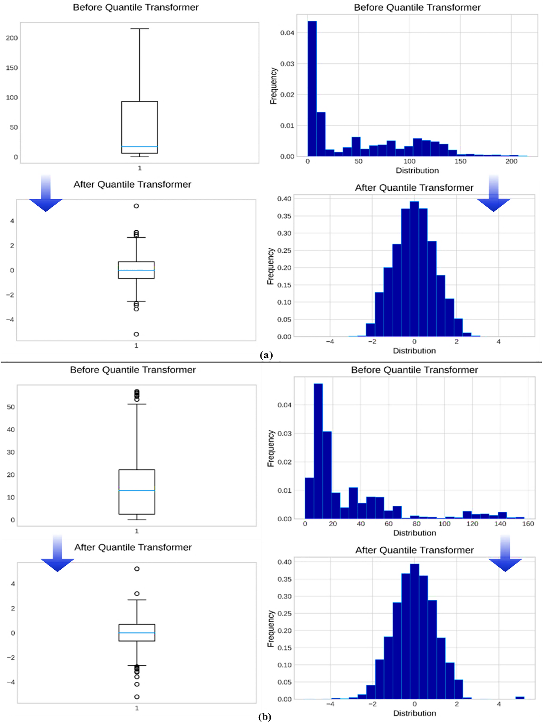
Figure 1: The distribution of data in the four datasets before and after applying the QT. The left side has box plots for examining outliers and skewness for 1st and 3rd wells data before and after the transformation ((a) represents TK908DH well data and (b) is the TK922H well data). After applying QT processing, the data distribution becomes smoother and more regular; the values become closer
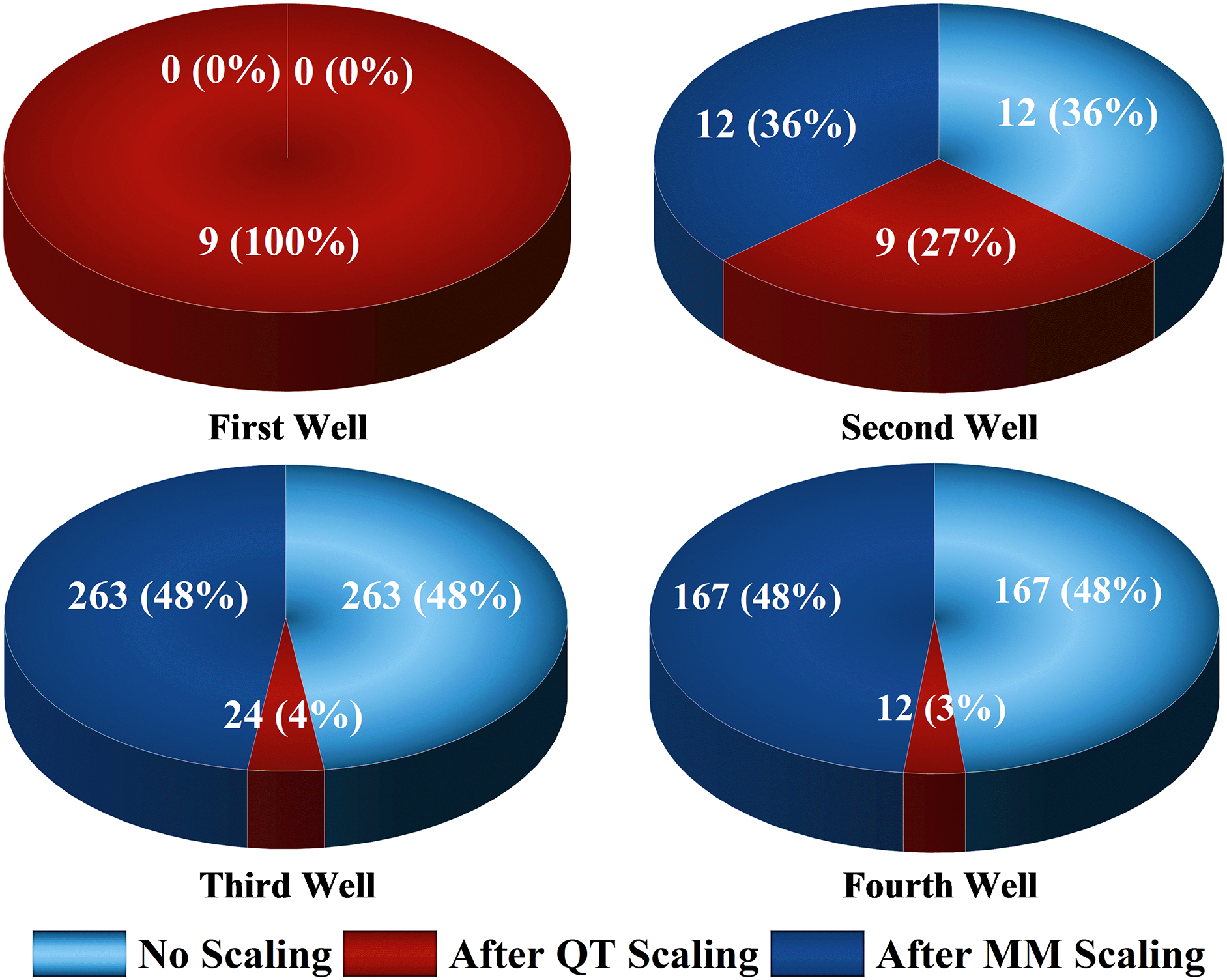
Figure 2: The number of outliers in each dataset, without scaling, after using MinMax scaling and quantile transformation
Before defining transfer learning, let us go through the concepts of a domain and a task. The domain
The task (
Transfer learning is the operation to improve the target objective function (
The components of LSTM are cell state (CS) and three gates (input gate, output gate, and forget gate). The gates are different neural networks to decide which information is allowed in the cell state. Cell state is the most critical part of LSTM, and it is a path to carry relevant information throughout the processing of the sequence; it is the horizontal red line in Fig. 3. The operation steps in LSTM are as follows: Firstly, the forget gate works to decide which information to omit before passing it to the cell state as follows:
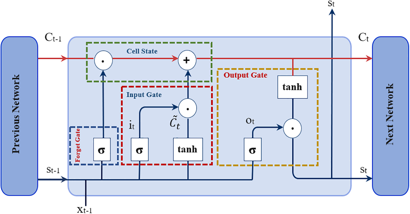
Figure 3: LSTM network with the various gates
The second step contains two portions to determine which correct data to pass into the CS, based on its importance. The first portion is the input gate (
Then getting the current new data of cell state as:
Finally, generate the output by passing new cell state data into the tanh function to get values between −1 and 1. After that, multiply these values with the output of the sigmoid gate (
In which, U indicates the input weight, W represents the recurrent weight, and b represents the bias, which here = 0. More so, f indicates the forget gate, where C represents the CS, o indicates the output gate, h represents the hidden state, and t represents the time step. Moreover,
3.4 Gated Recurrent Units (GRU)
The Gated Recurrent Units (GRU) was introduced by Cho et al. [25] to address the vanishing gradient problem of RNNs. The GRU is a variant of the LSTM, with fewer gates than the conventional LSTM. Thus, GRU requires less computation cost [13]. Fig. 4 shows the structure of the GRU network.
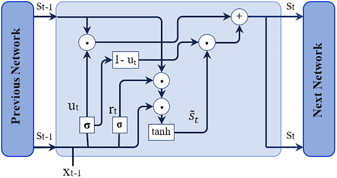
Figure 4: The structure of GRU
The first gate of the GRU is called the update gate. It employs the sigmoid function for scaling the outcomes between 0 and 1 to determine which values are selected to be transferred to the next step and eliminate the vanishing gradient problem.
The gate’s function is to prevent unwanted or unrelated values from being passed to the next operation.
In case of
The rest gate is used to store the corresponding values. This is done by multiplying the results with st−1 (previous state values). The results are then combined with the current input values before being passed to the tanh operation. The tanh function output is fed into the last step.
The final step is employed to obtain to get the network’s final results as the following:
3.5 The Transfer LSTM to GRU Model
Fig. 5 depicts this study’s structure, consisting of three stages and two parts. The initial stage is to collect data and remove any unwanted values, such as nulls and zeros. The second stage is comprehending each dataset’s data distribution well enough to prepare properly. Training the TLTG model is the third stage. The TLTG is a sequential model contains two parts. As is well known, LSTM is an effective method for forecasting time series due to its ability to retain longer series in its memory; this is detailed in Section 3.3; hence, the first part contains two LSTM layers. Before feeding the output of the first part to the next part, the freezing operation works to keep all the weights of the previous part. The second part contains six layers: two GRU layers, two batch normalization layers, and two fully connected layers (FC) (Fig. 5).
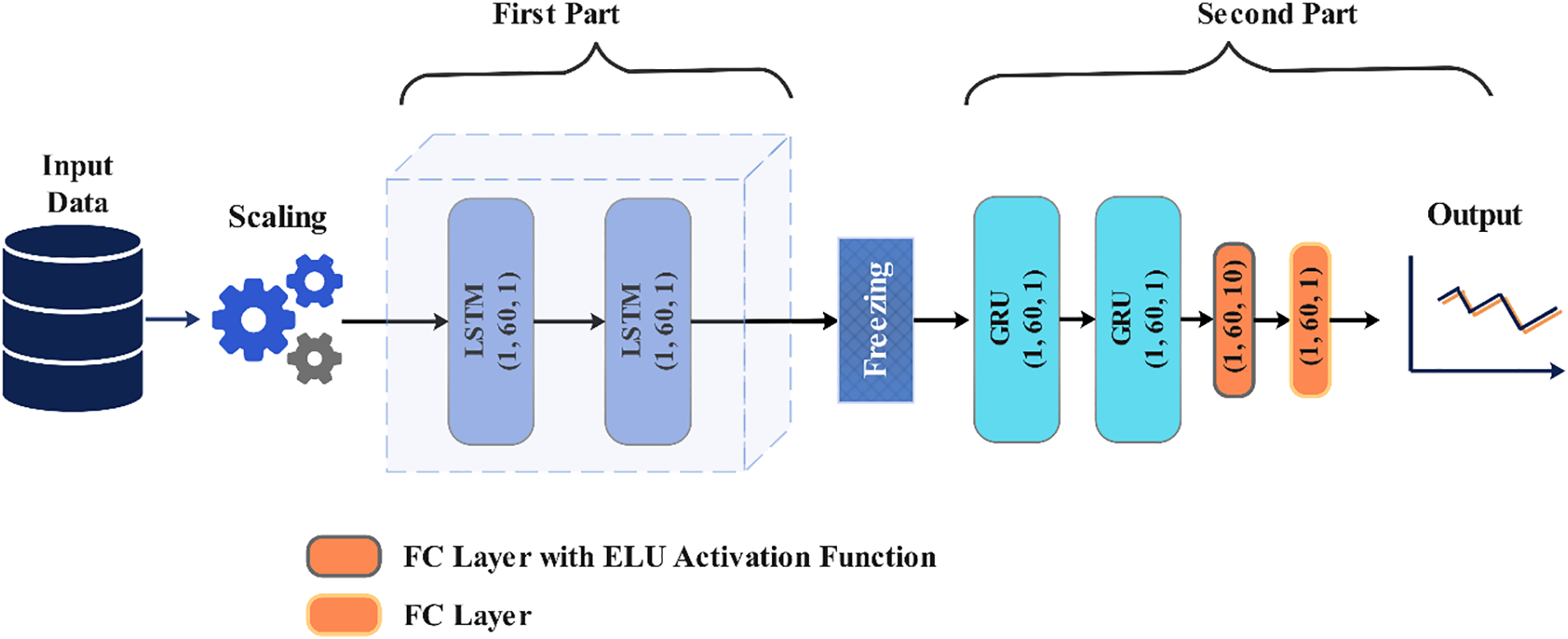
Figure 5: The model structure of this study
This part has two LSTM layers, one batch data entry from the bottom to the top of the LSTM model. Each cell state (CS) receives one batch of data inserted into the first layer of the LSTM, and the input gate accepts the data and processes it with the other LSTM gates, as mentioned before. The CS of the bottom LSTM returns the output data as the input data of the next layer and passes the output data to the next CS as short-term memory in the same layer. The final step returns a sequence of data, which is the output of the LSTM. Since LSTM has more gates than GRU, that enables it to analyze more complex data. Finally, the output of this part is transferred to the next part of processing to enhance the feature extraction and get the results.
3.5.2 Second Part of the Model
The second part retrains the first part’s weights with the input data and stops the backpropagation update in the first part (frozen), which helps avoid performance loss associated with training a deep network on a small dataset. Instead, performance is enhanced by updating the output based on feedback from the loss function in this part (second part). To achieve this, the layers in the first part are frozen to prevent weight changes. Consequently, weight updates and backpropagation occur only in the second part, without affecting the first part.
The two layers of GRU work to improve and enhance the output by updating the weights of this part according to the input data and the first part’s weights, which leads this part to choose the best weights. The GRU method is suitable for simple data with no complex distribution or frequency. It is a less complicated computation than LSTM and has a long memory. The output of GRUs is fed into the sequence of fully connected layers (FC). The first layer of FC uses the exponential linear unit (ELU) activation function,
All experiments were conducted on a 64-bit Windows 10 PC with 128 GB of RAM, 89 GB of GPU space, and Python as the programming language (Keras and Tensorflow).
This study uses datasets of four wells. Datasets are provided from the Tahe oil field in China. The data wells were collected daily from the beginning of 2004 to the end of 2014 from many different wells [26,27]. The first well (TK908DH) includes 3807 days from 31 May 2004, to 15 November 2014. The second well (T912CH) has 2653 days of records from 16 July 2007, to 15 November 2014. The third well (TK922H) has more records than the second, which is 3355 days from 04 September 2005, to 15 November 2014. Furthermore, the last oil well (TK935) has less data, which is 2003 days of records from 04 November 2008, to 15 November 2014, as shown in Fig. 6. The description of the main wells datasets is in Table 1.
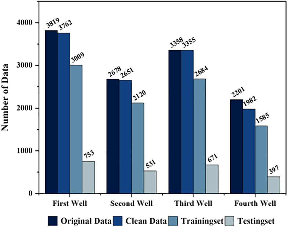
Figure 6: The number of recorded data in the four wells, the original data is the whole data with unacceptable data. Clean data is after removing all unacceptable data. Also, the size of the training and the testing set of each dataset
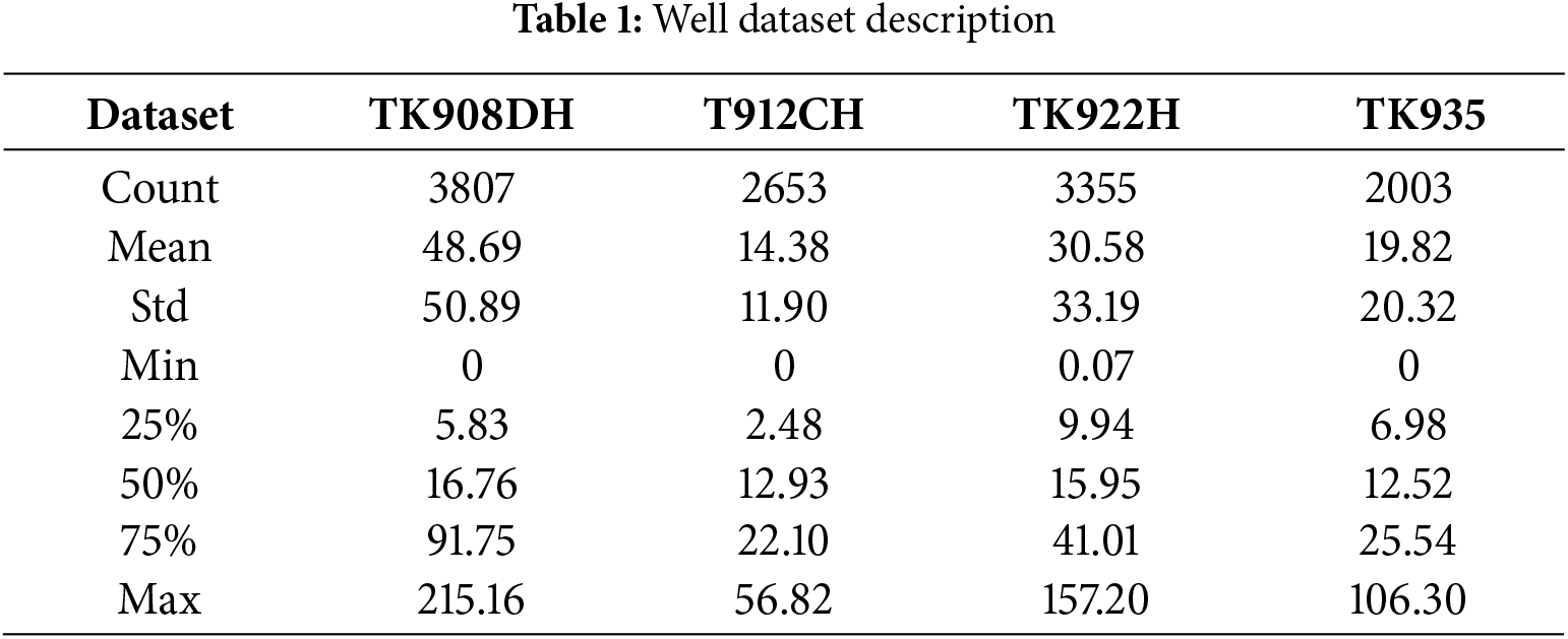
All datasets have unacceptable values like zeros or null values, so the first step was to clean the datasets. The size of each dataset is reduced, as can be seen in Fig. 6. Figs. 1 and 2 show the descriptions of values in each dataset and the outliers. The number of outliers is zero for the first well dataset, 12 for the second well dataset, 263 for the third well dataset, and 167 for the last well dataset.
This study divided the dataset into training and testing, 80% as a training set and 20% as a testing set. Additionally, mean squared error (MSE) was used during the training time as a loss function to improve forecasting and accuracy, and Adam was the optimizer. The epoch number and batch size are 10 and 1.
Mean Absolute Error (MAE), Root Mean Square Error (RMSE), Root Mean Square Percentage Error (RMSPE), and Coefficient of Determination (R2) are applied to assess the model efficiency.
where
4.3 Experimental Results and Comparisons
If the dimension of dataset values is large, the training becomes more complicated. The figures in this section show different distribution values for each dataset and different value dimensions between the sequence’s beginning and ending values, which means this study deals with different kinds of datasets.
A. Comparison with Different Preprocessing
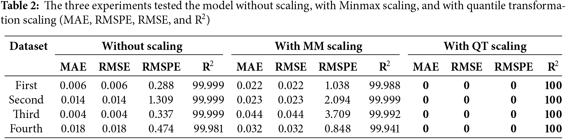
After cleaning the datasets from all zeros and unacceptable data like null and missing values, this study used three different kinds of preprocessing on the four datasets (clean data) before feeding them into the training network. There are three experiments: the first was without preprocessing methodologies, which did not use any scaling method to transfer the data to a different shape. In the second experiment, MM scaling was used as a preprocessing. The third experiment used Gaussian transformation (QT) to see the results of each experiment and figure out the best way to deal with outlier values and skewed distribution, as shown in Table 2.
The Transfer LSTM to GRU model (TLTG) has two sequential models, and its structure is in Fig. 5. The model has two LSTM layers with one unit. The second one takes the output of the first model with the input data into the second model after freezing the weight of the first part to deny retraining them again in the second part. The second model, or the second part of the TLTG, includes two GRU layers and one FC layer with an ELU activation function and ten units. The input training set was fed into the first part after going through the scaling process and splitting the dataset; the window size of the input data is 60.
The two layers of GRU in the second part optimize the last results of this TLTG model and extract the best weight according to the input data and the output of the first part. GRU has a lower computation cost than LSTM and a large memory, which helps to increase accuracy and reduce performance time. The trained output of these layers was fed into a sequence of fully connected layers (FC) with an ELU activation function to optimize the result more, avoid overfitting, and speed and normalize the training. The second FC has only one unit to provide the final output. Fig. 5 shows the model structure.
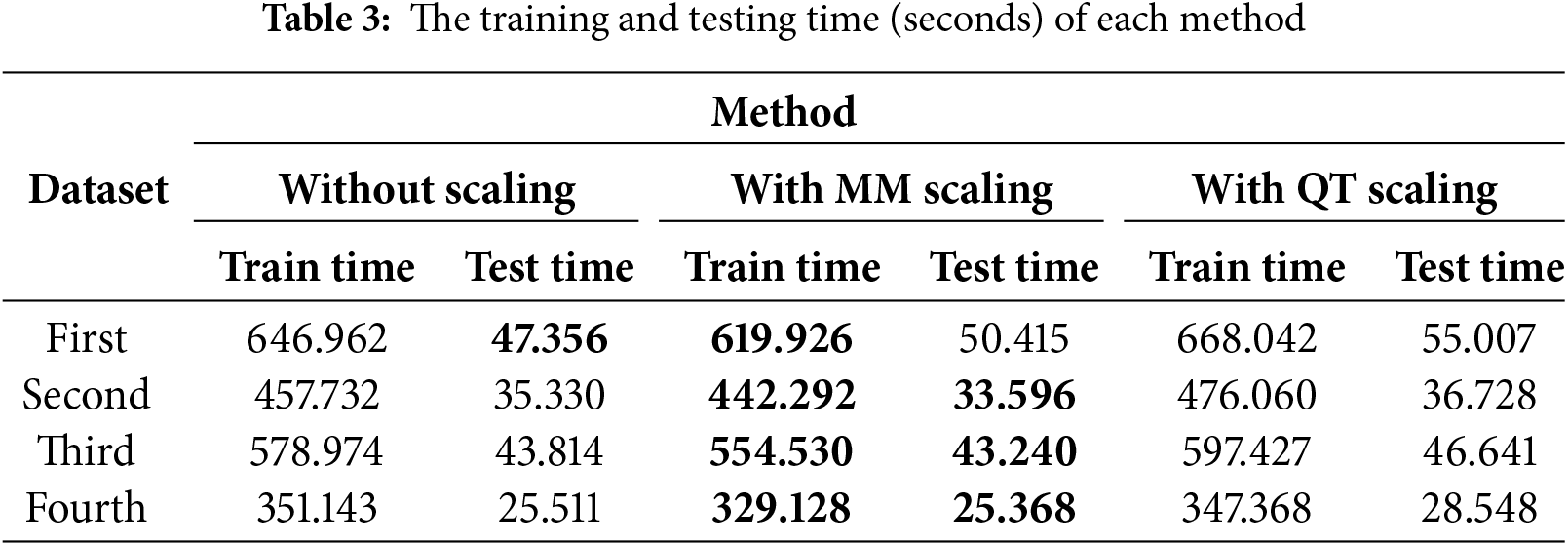
From Table 2, the results of QT scaling (Eq. (4)) have the best accuracy because the Gaussian transformation redistributes the input data and reduces outlier and skewed values; their distribution becomes more normal, as can be seen in Fig. 1. Without using any scaling operation, we also obtained better results than using the MM scaling (Eq. (1)) because, after using the MM scaling, the input data had more negative values besides the existence of outliers and skewness, which complicated the training more and obtained less accuracy. The MM scaling sped up the training and the tasting time more than the time of the QT method used, as seen in Table 3.
As shown in Table 2, the proposed model with QT scaling preprocessing (QT-TLTG) is the best, and it matches the original data better than others. QT scaling optimizes the data distribution before feeding it into the model. The model of this study runs to extract the perfect weights and more features by using the deep network. Combining and transferring learning between the two networks, two parts helps to reduce the loss. The TLTG model combines the deep network to extract more features and the shallow network to avoid losing and deal well with limited data. QT enhances the whole performance of the TLTG model by improving the input data distribution to be more normal, as detailed in Figs. 1 and 2. It shows the advantages of using transfer learning in deep models.
In summary, the QT scaling was successful, essentially creating a direct mapping between features and target values, allowing the TLTG model to produce perfect results. In contrast, MM scaling slightly degraded performance by altering the feature variances and did not improve the TLTG model’s results as effectively as QT scaling did. The Comparison with Other Models subsection shows the effect of the proposed framework (QT scaling with TLTG model) compared with well-known forecasting models.
B. Comparison with Other Models
This study compared its results with seven different models to see the efficiency of the TLTG model. These models are autoregressive integrated moving average (ARIMA), recurrent neural network (RNN), convolutional neural network-LSTM (CNN-LSTM), long short-term memory (LSTM1), gated recurrent units (GRU1), two LSTM (LSTM2), two GRU (GRU2), and LSTMGRU.
The ARIMA is one of the old methods for time-series predictions [22]. The CNN-LSTM model consists of two one-dimensional CNN (1D-CNN) layers with 60 filters, the kernel size is five, and the ReLu activation function. The third layer is LSTM, with 60 units. Then, two dense layers (FC layers) with (30, 10) units each and the ReLu activation function. The last layer is dense, with one unit for the output and final results. The RNN model comprises two layers of RNN, each followed by a 30% dropout layer. The GRU1 model is a GRU layer. In the LSTM1 model, there is only one LSTM layer. In contrast, the GRU2 model consists of two GRU layers followed by a 30% dropout layer. Similarly, the LSTM2 model contains two layers of LSTM instead of one, plus a 30% dropout layer after each layer to accelerate processing and prevent if there is any overfitting. The LSTMGRU model has the same structure of the TLTG models but without transferring, one block. Two LSTM layers (1, 60, 1), two GRU layers (1, 60, 1), one FC with ELU activation function, and the output layer (FC). It also used MSE loss function and Adam optimizer.
All models are sequential models except the ARIMA method. The mean squared error is the loss function in these sequential models, and Adam is the optimizer. The unit number is one, and the window size is 60. Except for the GRU1 and LSTM1 models, which trained with the actual values without any preprocessing, the other sequential models scaled the input data using MinMax scaling. The number of trainable parameters in each model is in Fig. 7.
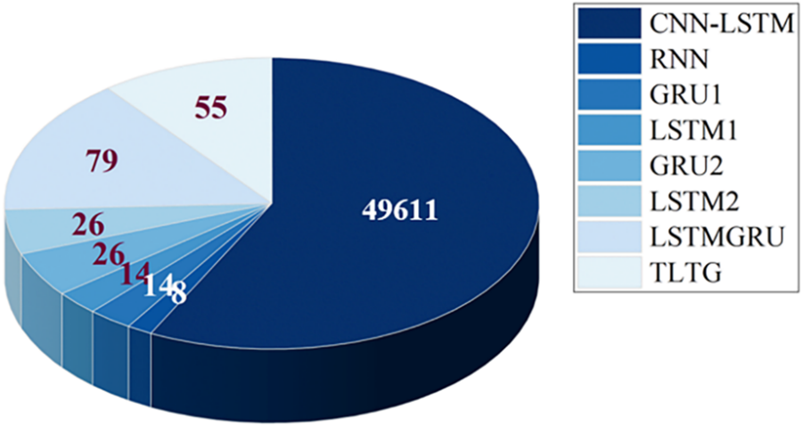
Figure 7: The trainable parameter number in each model
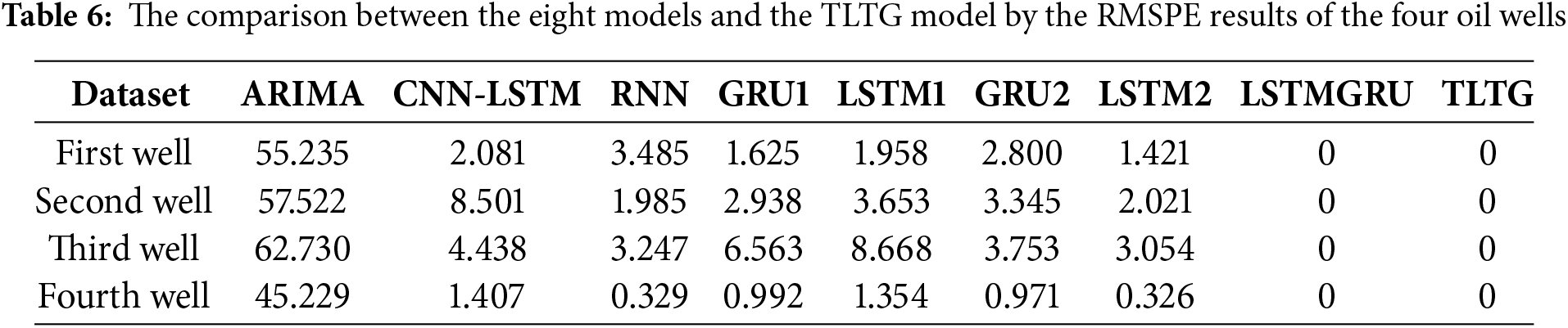
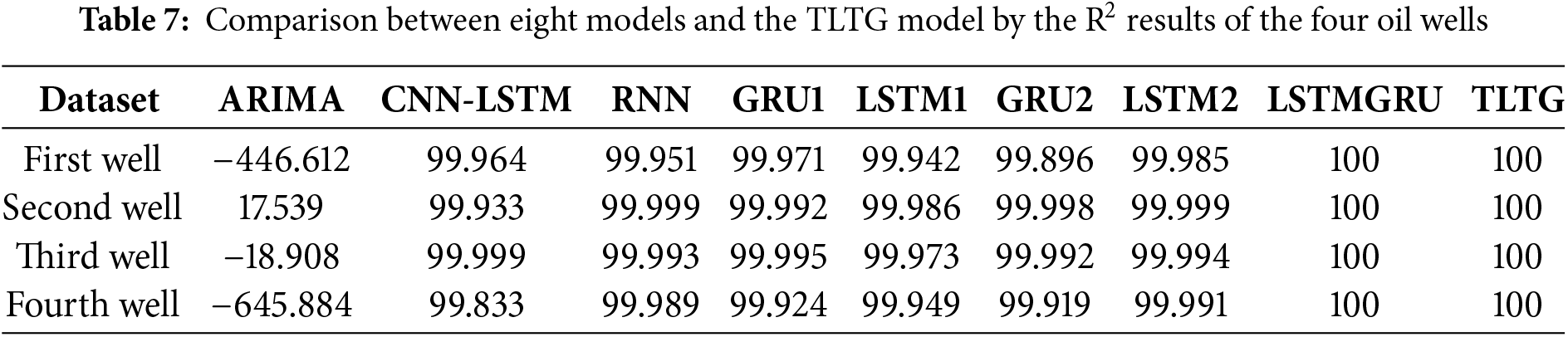
As shown in Tables 4 to 7, ARIMA is a simple method, so it achieved the lowest accuracy among all models, likely due to its limitations in handling complex and non-linear data distributions. Because the CNN-LSTM model can combine convolutional feature extraction with sequential learning, it achieved a good performance, particularly on the first and third wells. The same with the RNN model; it was also slightly less consistent across all datasets compared to the others. So, the RNN model has a limited ability to manage complex time dependencies in the data. The GRU model showed lower computational cost compared to the LSTM model. Even though the GRU1 model with a single GRU layer outperformed the GRU2 model with two GRU layers and the LSTM1 model, evidencing that deeper architectures do not always guarantee better performance and may lead to overfitting; as seen in Table 7, the R2 is higher in some cases.
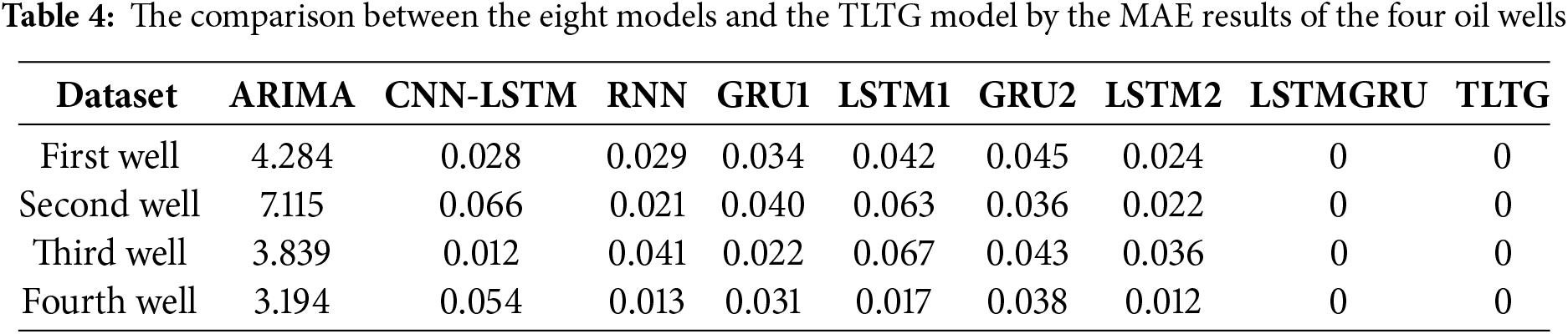
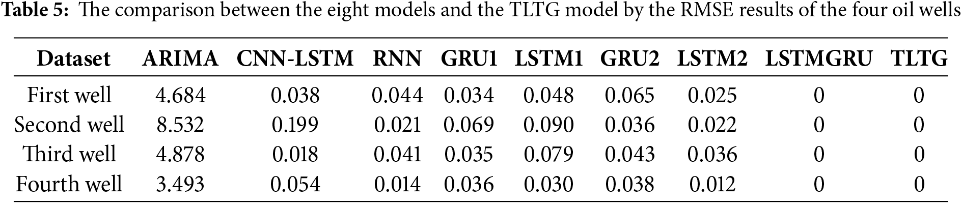
The LSTM-based models, including LSTM1 and LSTM2, had slightly higher MAE values than the GRU1 and GRU2 models, highlighting that GRUs may be better suited for handling smaller datasets with lower computational complexity. However, the hybrid LSTMGRU model achieved competitive results for all datasets, reflecting the benefit of combining LSTM and GRU in a sequential framework to provide a suitable and flexible model for many different data distributions.
The TLTG model extracts input data features in-depth without incurring an additional loss. Consequently, it yields the best outcomes, whether MM scaling or QT preprocessing is utilized. Figs. 1 and 2 illustrate how successfully QT preprocessing redistributes the data and improves it by minimizing the number of outliers and skewness, which was the aim of our analysis. The QT preprocessing assists the TLTG model in increasing the precision of all datasets. The results of the LSTMGRU and TLTG models with all four datasets are presented in Tables 4 through 7, and it is easy to deduce that these models performed the best.
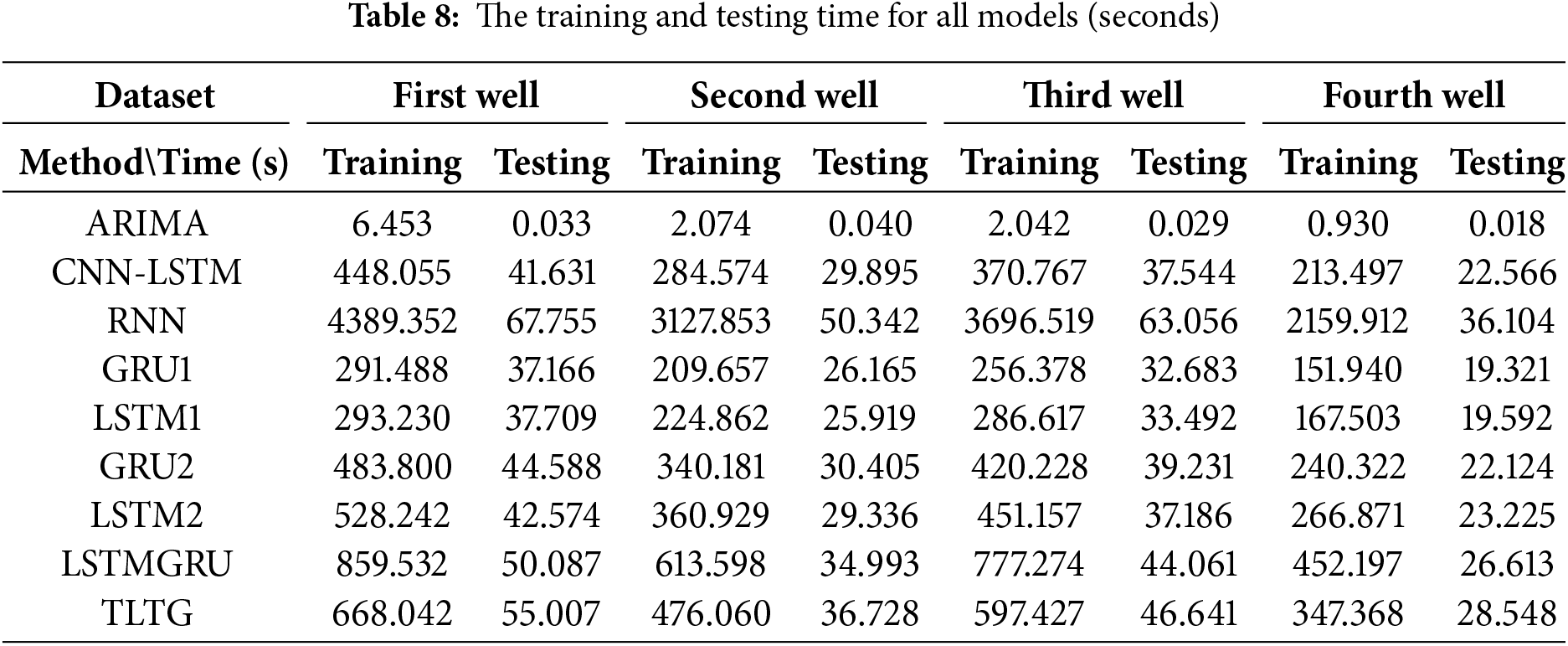
The fastest sequential model was the GRU, whereas the slowest one was the RNN model. Although the CNN-LSTM model has the largest parameter number (Fig. 7), the two layers of the CNN worked to reduce the size of the generated feature maps during the training time. That helped to accelerate the processing of the CNN-LSTM model. The TLTG model was faster than the RNN and LSTMGRU models, which was 200 s faster than the LSTMGRU model (Table 8). The difference between them is enormous; this is the advantage of using transfer learning inside the TLTG model. The TLTG model provided the best performance, highest accuracy, and adequate processing time (Tables 4–8).
The TLTG model combines the deep network to extract more features and the shallow network (the first part of the TLTG model) to prevent data loss and deal well with limited data by moving the weights of the first section to the next. Therefore, the second part modifies and trains the network based on the input data and weights of the first part to achieve optimal outcomes. Figs. 8 to 11 clearly demonstrate that our TLTG model has been highly effective at extracting and forecasting the time series of all datasets. Consequently, the suggested TLTG model surpasses all comparative approaches for all datasets in the Tahe field, proving the method’s superiority over the eight other methods, including LSTMGRU.
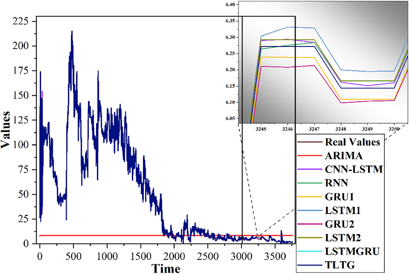
Figure 8: Comparison of the original and predicted data by the TLTG model and the other eight models for the first dataset
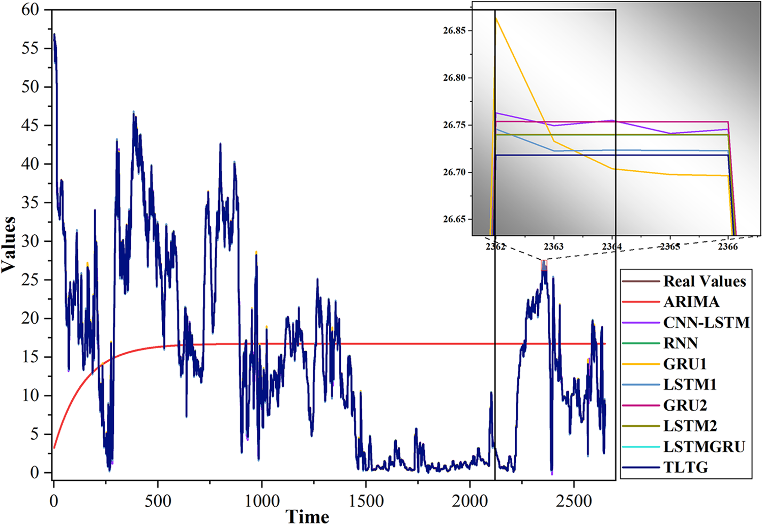
Figure 9: Comparison of the original and predicted data by the TLTG model and the other eight models for the second dataset
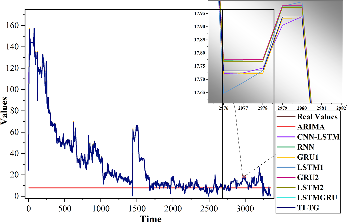
Figure 10: Comparison of the original and predicted data by the TLTG model and other eight models for the third dataset. The enlarged side image shows the differences between the models clearly
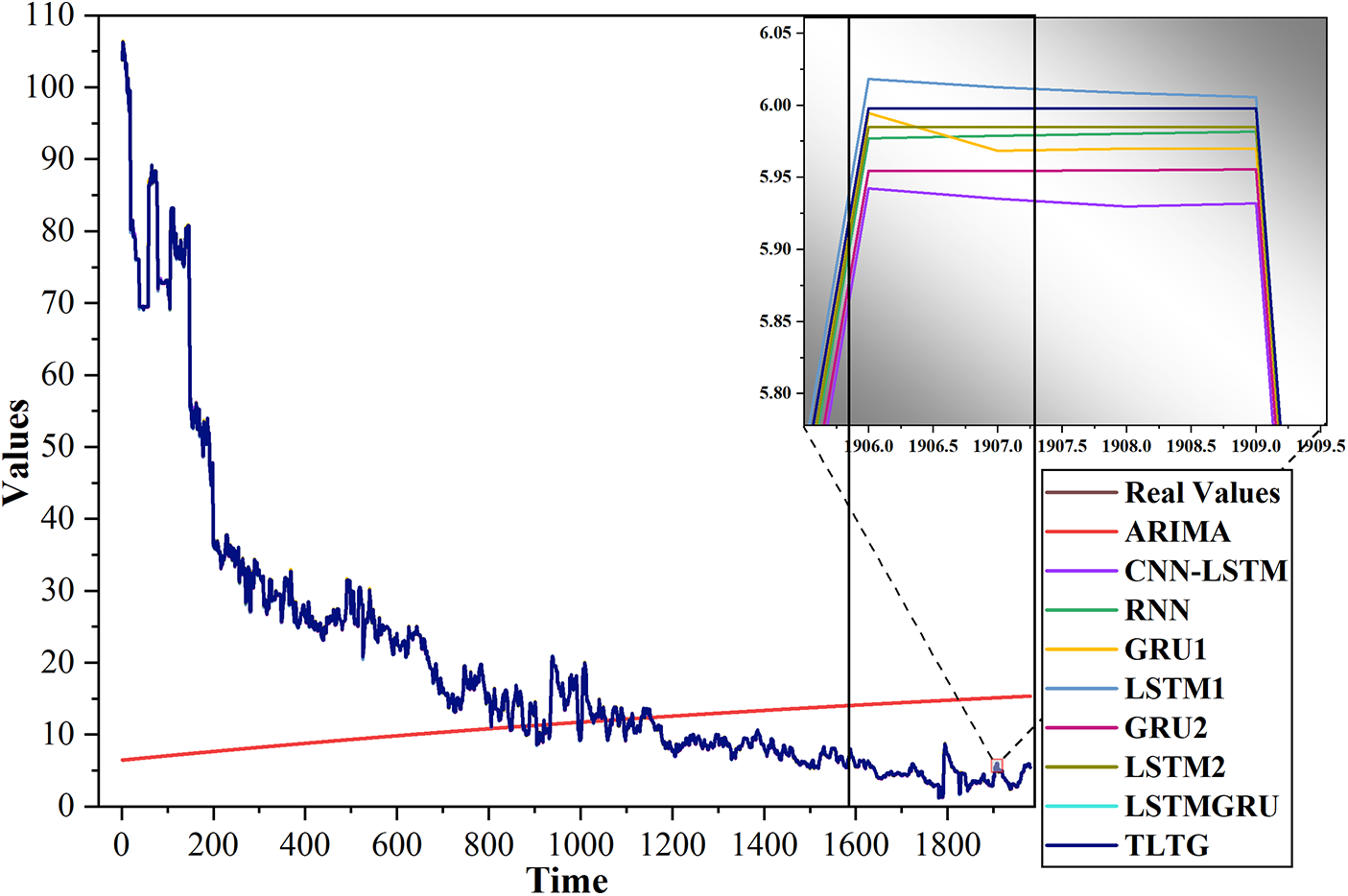
Figure 11: Comparison of the original and predicted data by the TLTG model and the other eight models for the fourth dataset
Because of the findings of the study, we can say the framework (TLTG) can accurately forecast oil production using small, complex datasets and can significantly improve reservoir management strategies. By addressing challenges such as outlier values, skewed data distributions, and computational efficiency, the TLTG model offers a robust tool for improving decision-making in resource allocation.
5 Other Comparison and Testing
Since the datasets used in this study are not publicly available, the performance of the proposed Transfer LSTM to GRU (TLTG) model was evaluated using widely recognized time-series datasets that are publicly licensed. A summary of these datasets is provided in Table 9. To ensure scientific rigor and facilitate comparisons, our study benchmarked the TLTG model against existing approaches that used these public datasets, demonstrating its robustness across diverse data distributions.

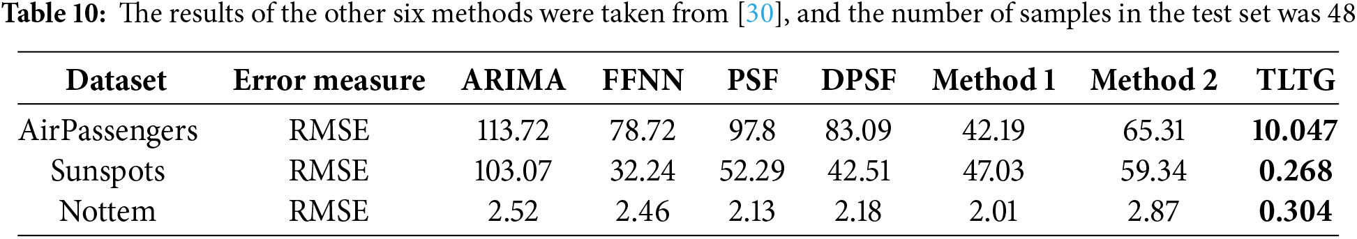
Specifically, reference [28] provides a comparative study that utilized the AirPassengers, Sunspots, and Nottem datasets, and reference [29] used the Lynx dataset. Consistent with their methodology, we used the last 48 records as the test set and the remaining records as the training set. Both studies employed Root Mean Squared Error (RMSE) as the evaluation metric, allowing for a direct performance comparison, as summarized in Table 10.
Similarly, reference [28] adopted a different evaluation approach by splitting the AirPassengers, Sunspots, and Lynx datasets into 80% for training and 20% for testing, using Mean Absolute Error (MAE) as the performance measure. We followed this setup to ensure alignment and comparability, with the results outlined in Table 11. Fig. 12 illustrates the data distribution across these datasets, further validating the robustness of our methodology.
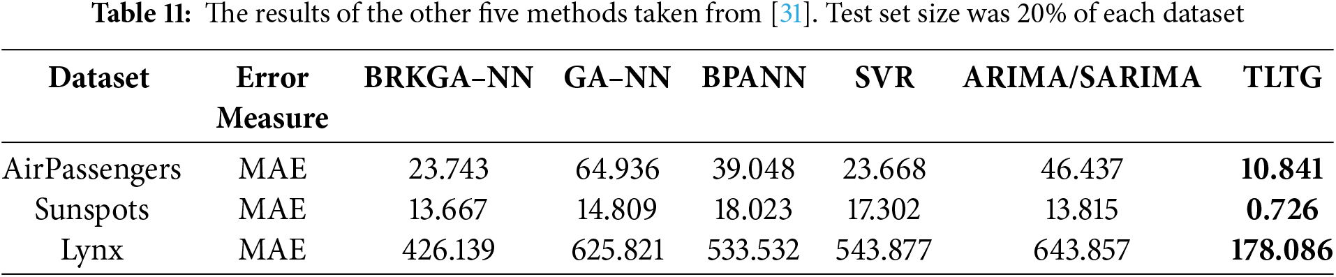
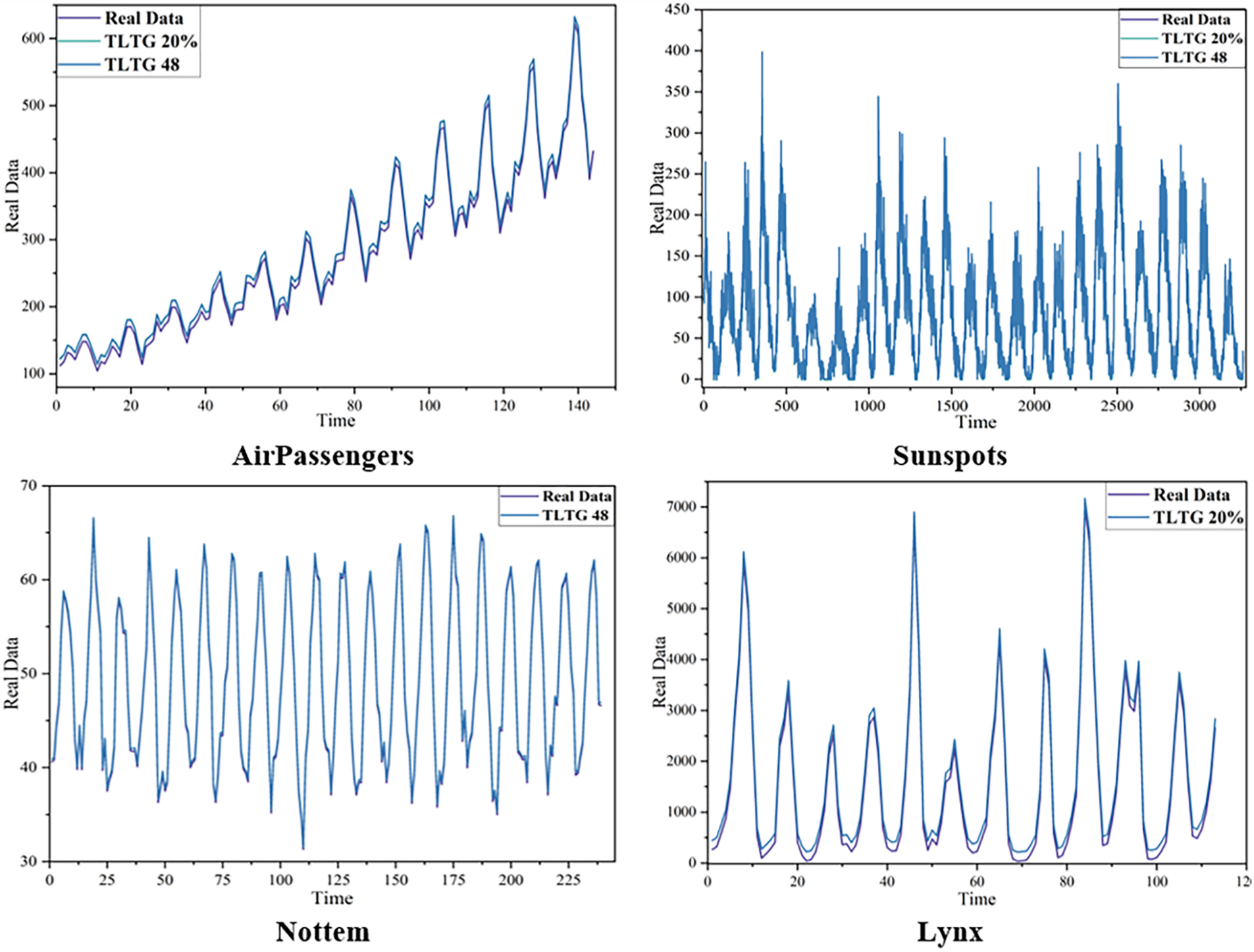
Figure 12: The data used to validate the proposed method (TLTG)
Tables 10 and 11 were extracted verbatim from [30,31], and we trained the identical datasets with the same split of the training set and test set in both studies. Then, the TLTG method results were added to Tables 10 and 11. From the same Tables, it can be observed clearly that the TLTG model is demonstrably superior to all other approaches.
The TLTG outperforms the best-compared approach, Method 1 in Table 10 from [30], by 32 times, and SVR in Table 11 from [31] by 13 times. Fig. 12 depicts the TLTG results for the four different datasets.
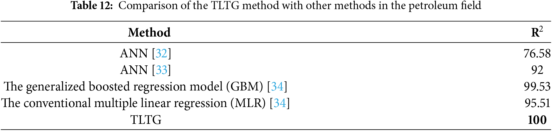
In petroleum field studies, the results of the TLTG method were compared with previous oil prediction models in Table 12. As can be observed, the TLTG is the best and most flexible model with any data distribution.
This paper proposed a unique transfer LSTM to GRU (TLTG) model with QT preprocessing to enhance time series forecasting for four oil wells in the Tahe Field in China. The TLTG model enhances the results by transferring the output of the first part of the model to the second. Additionally, a Gaussian Transformation was applied before training to normalize the input data, enhancing overall performance. The experiments of the TLTG model demonstrated the following: 1) The TLTG model can provide high accuracy for the different datasets with different distributions. 2) By employing transfer learning, the model demonstrated exceptional capability in handling small and complex datasets. 3) Also, the transfer learning approach optimized the TLTG model’s training process, reducing computational complexity without compromising accuracy. The model proved that combining the advantages of deep and shallow networks helped achieve higher accuracy with fewer data. 4) The Gaussian transformation in the preprocessing stage provides a very effective way to deal with outlier values and skewness. 5) The results showed that the TLTG model outperformed all other state-of-the-art models compared with them. Future work will focus on further optimizing the performance time of the TLTG model while maintaining its high accuracy. Additionally, we plan to improve the preprocessing stage to enhance the data distribution and forecasting execution.
Acknowledgement: The authors would like to express their sincere gratitude to Ahamed Alalimi for providing the necessary resources for this study. We also acknowledge the contributions of everyone whose feedback significantly improved the quality of this work.
Funding Statement: The authors received no specific funding for this study.
Author Contributions: The authors confirm contribution to the paper as follows: Conceptualization: Dalal AL-Alimi, and Mohammed A. A. Al-qaness; Data curation: Dalal AL-Alimi; Formal analysis: Dalal AL-Alimi, and Robertas Damaševičius; Methodology: Dalal AL-Alimi; Software: Dalal AL-Alimi; Visualization: Dalal AL-Alimi; Validation: Robertas Damaševičius; Writing—original draft: Dalal AL-Alimi; Writing—review & editing: Robertas Damaševičius, and Mohammed A. A. Al-qaness. All authors reviewed the results and approved the final version of the manuscript.
Availability of Data and Materials: The data that support the findings of this study are openly available in GitHub at https://github.com/DalalAL-Alimi/TLTG (accessed on 26 December 2024).
Ethics Approval: Not applicable.
Conflicts of Interest: The authors declare no conflicts of interest to report regarding the present study.
References
1. Male F. Using a segregated flow model to forecast production of oil, gas, and water in shale oil plays. J Pet Sci Eng. 2019;180(9):48–61. doi:10.1016/j.petrol.2019.05.010. [Google Scholar] [CrossRef]
2. Liu W, Liu WD, Gu J. Forecasting oil production using ensemble empirical model decomposition based Long Short-Term Memory neural network. J Pet Sci Eng. 2020;189(2):107013. doi:10.1016/j.petrol.2020.107013. [Google Scholar] [CrossRef]
3. Bhardwaj S, Chandrasekhar E, Padiyar P, Gadre VM. A comparative study of wavelet-based ANN and classical techniques for geophysical time-series forecasting. Comput Geosci. 2020;138(1):104461. doi:10.1016/j.cageo.2020.104461. [Google Scholar] [CrossRef]
4. AL-Alimi D, AlRassas AM, Al-qaness MAA, Cai Z, Aseeri AO, Abd Elaziz M, et al. TLIA: time-series forecasting model using long short-term memory integrated with artificial neural networks for volatile energy markets. Appl Energy. 2023;343(7):121230. doi:10.1016/j.apenergy.2023.121230. [Google Scholar] [CrossRef]
5. Sagheer A, Kotb M. Time series forecasting of petroleum production using deep LSTM recurrent networks. Neurocomputing. 2019;323(3):203–13. doi:10.1016/j.neucom.2018.09.082. [Google Scholar] [CrossRef]
6. Abbasimehr H, Behboodi A, Bahrini A. A novel hybrid model to forecast seasonal and chaotic time series. Expert Syst Appl. 2024;239(1):122461. doi:10.1016/j.eswa.2023.122461. [Google Scholar] [CrossRef]
7. Clarkson CR, Williams-Kovacs JD, Qanbari F, Behmanesh H, Sureshjani MH. History-matching and forecasting tight/shale gas condensate wells using combined analytical, semi-analytical, and empirical methods. J Nat Gas Sci Eng. 2015;26:1620–47. doi:10.1016/j.jngse.2015.03.025. [Google Scholar] [CrossRef]
8. Kalra S, Tian W, Wu X. A numerical simulation study of CO2 injection for enhancing hydrocarbon recovery and sequestration in liquid-rich shales. Pet Sci. 2018;15:103–15. doi:10.1007/s12182-017-0199-5. [Google Scholar] [CrossRef]
9. Song X, Liu Y, Xue L, Wang J, Zhang J, Wang J, et al. Time-series well performance prediction based on Long Short-Term Memory (LSTM) neural network model. J Pet Sci Eng. 2020;186(2):106682. doi:10.1016/j.petrol.2019.106682. [Google Scholar] [CrossRef]
10. Tealab A. Time series forecasting using artificial neural networks methodologies: a systematic review. Futur Comput Informatics J. 2018;3(2):334–40. doi:10.1016/j.fcij.2018.10.003. [Google Scholar] [CrossRef]
11. Zhang Z, Moore JC. Autoregressive moving average models. In: Mathematical and physical fundamentals of climate change. Boston: Elsevier; 2015. p. 239–90. doi:10.1016/B978-0-12-800066-3.00008-5. [Google Scholar] [CrossRef]
12. Ning Y, Kazemi H, Tahmasebi P. A comparative machine learning study for time series oil production forecasting: ARIMA, LSTM, and Prophet. Comput Geosci. 2022;164(1):105126. doi:10.1016/j.cageo.2022.105126. [Google Scholar] [CrossRef]
13. Eren Y, Küçükdemiral İ. A comprehensive review on deep learning approaches for short-term load forecasting. Renew Sustain Energy Rev. 2024;189(1):114031. doi:10.1016/j.rser.2023.114031. [Google Scholar] [CrossRef]
14. LeCun Y, Bengio Y, Hinton G. Deep learning. Nature. 2015;521:436–44. doi:10.1038/nature14539. [Google Scholar] [PubMed] [CrossRef]
15. Edalatpanah SA, Hassani FS, Smarandache F, Sorourkhah A, Pamucar D, Cui B. A hybrid time series forecasting method based on neutrosophic logic with applications in financial issues. Eng Appl Artif Intell. 2024;129(2):107531. doi:10.1016/j.engappai.2023.107531. [Google Scholar] [CrossRef]
16. Bacanin N, Stoean C, Zivkovic M, Rakic M, Strulak-Wójcikiewicz R, Stoean R. On the benefits of using metaheuristics in the hyperparameter tuning of deep learning models for energy load forecasting. Energies. 2023;16(3):1434. doi:10.3390/en16031434. [Google Scholar] [CrossRef]
17. Wang J, Cao J, Yuan S. Shear wave velocity prediction based on adaptive particle swarm optimization optimized recurrent neural network. J Pet Sci Eng. 2020;194(5):107466. doi:10.1016/j.petrol.2020.107466. [Google Scholar] [CrossRef]
18. Nikitin NO, Revin I, Hvatov A, Vychuzhanin P, Kalyuzhnaya AV. Hybrid and automated machine learning approaches for oil fields development: the case study of Volve field, North Sea. Comput Geosci. 2022;161(4):105061. doi:10.1016/j.cageo.2022.105061. [Google Scholar] [CrossRef]
19. Lu J, Behbood V, Hao P, Zuo H, Xue S, Zhang G. Transfer learning using computational intelligence: a survey. Knowl-Based Syst. 2015;80:14–23. doi:10.1016/j.knosys.2015.01.010. [Google Scholar] [CrossRef]
20. Le T, Vo MT, Kieu T, Hwang E, Rho S, Baik SW. Multiple electric energy consumption forecasting using a cluster-based strategy for transfer learning in smart building. Sensors. 2020;20(9):2668. doi:10.3390/s20092668. [Google Scholar] [PubMed] [CrossRef]
21. Ye R, Dai Q. A novel transfer learning framework for time series forecasting. Knowl-Based Syst. 2018;156(6):74–99. doi:10.1016/j.knosys.2018.05.021. [Google Scholar] [CrossRef]
22. Liang B, Liu J, You J, Jia J, Pan Y, Jeong H. Hydrocarbon production dynamics forecasting using machine learning: a state-of-the-art review. Fuel. 2023;337(6):127067. doi:10.1016/j.fuel.2022.127067. [Google Scholar] [CrossRef]
23. Fernández A, García S, Galar M, Prati RC, Krawczyk B, Herrera F, Learning from imbalanced data sets. 1st ed. Cham: Springer International Publishing; 2018. doi:10.1007/978-3-319-98074-4. [Google Scholar] [CrossRef]
24. Raju VNG, Lakshmi KP, Jain VM, Kalidindi A, Padma V. Study the influence of normalization/transformation process on the accuracy of supervised classification. In: 2020 Third International Conference on Smart Systems and Inventive Technology (ICSSIT); 2020 Aug 20–22; Tirunelveli, India: IEEE. p. 729–35. doi:10.1109/ICSSIT48917.2020.9214160. [Google Scholar] [CrossRef]
25. Cho K, Van Merriënboer B, Gulcehre C, Bahdanau D, Bougares F, Schwenk H, et al. Learning phrase representations using RNN encoder-decoder for statistical machine translation. arXiv:1406.1078. 2014. [Google Scholar]
26. AlRassas AM, Al-qaness MAA, Ewees AA, Ren S, Abd Elaziz M, Damaševičius R, et al. Optimized ANFIS model using aquila optimizer for oil production forecasting. Processes. 2021;9(7):1194. doi:10.3390/pr9071194. [Google Scholar] [CrossRef]
27. Alalimi A, Pan L, Al-qaness MAA, Ewees AA, Wang X, Abd Elaziz M. Optimized random vector functional link network to predict oil production from tahe oil field in China. Oil Gas Sci Technol-Rev IFP Energies Nouv. 2021;76(3):1–10. doi:10.2516/ogst/2020081. [Google Scholar] [CrossRef]
28. Shende MK, Salih SQ, Bokde ND, Scholz M, Oudah AY, Yaseen ZM. Natural time series parameters forecasting: validation of the pattern-sequence-based forecasting (PSF) algorithm; a new python package. Appl Sci. 2022;12(12):6194. doi:10.3390/app12126194. [Google Scholar] [CrossRef]
29. Kokko H. Who is afraid of modelling time as a continuous variable? Methods Ecol Evol. 2024;15(10):1736–56. doi:10.1111/2041-210x.14394. [Google Scholar] [CrossRef]
Bokde ND, Tranberg B, Andresen GB. Short-term CO2 emissions forecasting based on decomposition approaches and its impact on electricity market scheduling. Appl Energy, 2020;281:116061. doi:10.1016/j.apenergy.2020.116061. [Google Scholar] [CrossRef]
31. Erzurum Cicek ZI, Kamisli Ozturk Z. Optimizing the artificial neural network parameters using a biased random key genetic algorithm for time series forecasting. Appl Soft Comput. 2021;102(6):107091. doi:10.1016/j.asoc.2021.107091. [Google Scholar] [CrossRef]
32. Iturrarán-Viveros U, Parra JO. Artificial Neural Networks applied to estimate permeability, porosity and intrinsic attenuation using seismic attributes and well-log data. J Appl Geophys. 2014;107(5):45–54. doi:10.1016/j.jappgeo.2014.05.010. [Google Scholar] [CrossRef]
33. Zolotukhin AB, Gayubov AT. Machine learning in reservoir permeability prediction and modelling of fluid flow in porous media. IOP Conf Ser: Mater Sci Eng. 2019;700(1):012023. doi:10.1088/1757-899X/700/1/012023. [Google Scholar] [CrossRef]
34. Al-Mudhafar WJ. Integrating well log interpretations for lithofacies classification and permeability modeling through advanced machine learning algorithms. J Pet Explor Prod Technol. 2017;7(4):1023–33. doi:10.1007/s13202-017-0360-0. [Google Scholar] [CrossRef]
Cite This Article
 Copyright © 2025 The Author(s). Published by Tech Science Press.
This work is licensed under a Creative Commons Attribution 4.0 International License , which permits unrestricted use, distribution, and reproduction in any medium, provided the original work is properly cited.
 Downloads
 Citation Tools