A Boundary-Type Meshless Method for Traction Identification in Two-Dimensional Anisotropic Elasticity and Investigating the Effective Parameters

1  Introduction

Determining the traction applied to an edge of an anisotropic body is very important in structural health monitoring and optimal design of structures. The traction applied to a body cannot usually be measured directly but should be determined using inverse methods, in which displacement or strain measurements are taken at several points on the body. In direct problems, the boundary conditions, the material properties, and the applied loads are known and the displacement, strain, and stress fields in the domain are calculated by solving the problem. In inverse problems, the boundary conditions, the material properties or the applied loads are not known, and by using an inverse method and measured data, the unknowns are calculated. Inverse problems may be ill-posed [1] and are usually more difficult to solve than direct problems.

Inverse problems related to anisotropic elastostatic problems have been the subject of intense research in recent decades. Some researchers have studied the identification of elastic constants of anisotropic solids. Van Hemelrijck et al. [2] presented an inverse finite element method based on a static biaxial test for the identification of two-dimensional (2D) elastic constants of composite laminates. They used full-field strain measurements in their inverse method. Hematiyan et al. [3] presented an inverse method based on the boundary element method for the identification of 2D anisotropic elastic constants. They employed displacement measurements from more than one elastostatic test to overcome the ill-posedness of the inverse problem. An inverse finite element method for determining in-plane orthotropic elastic constants of 2D solids was presented by Nigamaa et al. [4]. They employed full-field strain measurements in the inverse analysis. Chen et al. [5] presented a method based on the singular boundary method for the identification of elastic constants of orthotropic materials. They used measured data obtained from measurement points on the boundary of the problem in the inverse analysis. Hematiyan et al. [6] presented an inverse meshless radial interpolation method for the identification of all 21 elastic constants of three-dimensional (3D) generally anisotropic solids. They used strain measured data obtained from several simple elastostatic tests to find the unknown elastic constants. Smyl et al. [7] presented an inverse method for identifying elastic properties of inhomogeneous orthotropic materials. They used displacement field obtained from digital image correlation through quasi-static elasticity imaging in their method. Mei et al. [8] proposed an inverse method for determining inhomogeneous elastic parameters of two-dimensional orthotropic materials using a finite number of displacement measurements. They employed an iterative inverse algorithm along with the finite element method in their approach. Another inverse method based on the finite element method for the identification of elastic constants of 2D orthotropic materials was proposed by Kim et al. [9]. They used a specimen with an elliptic hole and full-field measurements in their inverse method. Zhang et al. [10] presented a machine learning model based on a modified radial basis function neural network to determine 21 elastic constants of anisotropic additive-manufactured solids. They utilized the Young’s modulus and the shear modulus values of samples in different orientations to predict the elastic constants. Recently, Hematiyan et al. [11] proposed an inverse method of fundamental solutions (MFS) for the identification of 2D anisotropic elastic constants of solids.

Identification of boundary conditions in isotropic elasticity has been the subject of many studies (e.g., [12–16]); however, this type of inverse problem for anisotropic materials has received less attention. Comino et al. [17] proposed an iterative inverse method based on the boundary element method for the identification of boundary conditions in 2D anisotropic elasticity. They also investigated the effect of the amount of measurement error on the accuracy of the solution. Zhang et al. [18] developed a non-iterative inverse method based on the meshless local Petrov-Galerkin method for inverse analysis of isotropic and anisotropic solids. They assumed that a portion of the boundary is over-determined, i.e., both the traction and displacement are prescribed on that portion, while the boundary condition on another portion of the boundary is unknown. A similar inverse Trefftz method based on the Stroh formalism was proposed by Zhang et al. [19].

The MFS, which is a well-known boundary-type meshfree method, is very suitable for inverse analysis of engineering problems because it is computationally efficient and simple to program. Moreover, various boundary conditions can be implemented in the MFS without any integration. The MFS has been widely used for inverse analyses [20]. Although the MFS has not been employed for traction identification in anisotropic elasticity, it has been widely employed for boundary condition identification in isotropic media. Marin [21] proposed an iterative inverse MFS for the identification of the condition on a portion of the boundary of an isotropic domain, while both the traction and displacement on another portion of the boundary were prescribed. He used the Tikhonov regularization method in the inverse analysis and chose an appropriate value for the regularization parameter using the generalized cross-validation criterion. Moreover, Marin et al. [22] proposed another inverse MFS based on the fading regularization method for solving the same inverse problem. Marin et al. [23] proposed a non-iterative MFS for the identification of boundary conditions on a part of the boundary of 2D and 3D isotropic elastic domains. They considered over-prescribed boundary conditions on the remaining boundary and examined some regularization methods in the inverse analysis.

A review of previous works shows that the MFS has been widely used for various inverse problems in isotropic media. Moreover, it is observed that the MFS has been employed for the identification of elastic constants of anisotropic materials; however, neither the MFS nor other boundary-type meshless methods have yet been used for the identification of traction on the boundary of anisotropic bodies. Boundary-type meshless methods are more attractive than domain-type methods because they require less effort from the user. In this paper, an inverse MFS for the identification of traction on a part of the boundary is presented. Measured displacements or strains taken at several points in the domain or on the boundary are used in the inverse method. The effects of important parameters such as the number of measurements, the location of measurement points, the amount of measurement error, and the type of the measurement (displacement or strain) on the results are also investigated.

2  The MFS for 2D Anisotropic Elasticity

The MFS is a boundary-type meshless method that has been widely employed for the analysis of linear problems. It is a semi-analytical method, in which the governing equations are exactly satisfied in the problem domain, while the boundary conditions of the problem are satisfied at a number of collocation points on the boundary. The MFS was introduced as a numerical method more than four decades ago [24]. An overview of the MFS can be found in [25]. Since the MFS is an efficient computational method, it has been used for the analysis of various problems. A few examples include the use of the MFS in the analysis of Poisson’s equation [26,27], elastostatic problems [28,29], isotropic thermoelasticity [30,31], anisotropic thermoelasticity [32], elastodynamic problems [33,34], and plate bending problems [35–37]. A variation of the MFS, called the localized method of fundamental solutions, has also been presented, which can be more efficient for large scale problems [38,39]. In the finite element method, which is a very popular method, it is required to discretize the domain of the problem, which can lead to difficulties in some problems. In domain-type meshless methods (e.g., [40,41]), there is no need to define any elements; however, it is necessary to define a sufficient number of nodes in the domain of the problem. The MFS compared to the finite element and meshless methods, is more attractive because it is a boundary-type meshless method, and there is no need to consider any internal nodes or elements with this method. The boundary element method (e.g., [42,43]) is also a well-known boundary-type method that does not require domain discretization. The MFS compared to the boundary element method, is simpler because the MFS is an integral-free method, while various singular integrals must be computed in the boundary element method.

In this section, the MFS for 2D anisotropic elasticity is briefly described. The unknowns in the 2D elasticity problem are the displacements in the x1 and x2 directions, i.e., u1 and u2, the in-plane strains ε11, ε22, and ε12, and the in-plane stresses σ11, σ22, and σ12. The governing equations of the problem are equilibrium relations, strain-displacement equations, and stress-strain relations [44]. The equilibrium equations are:

∂σ11∂x1+∂σ12∂x2=0,(1)

∂σ12∂x1+∂σ22∂x2=0.(2)

The strain components in terms of the displacement components can be expressed as follows:

ε11=∂u1∂x1,ε22=∂u2∂x2,ε12=12(∂u1∂x2+∂u2∂x1).(3)

For an anisotropic material, the strain components in terms of the stress components can be written as follows:

{ε11ε222ε12}=[a11a12a16a21a22a26a61a62a66]{σ11σ22σ12},(4)

where aij represent the elastic compliance coefficients of the anisotropic material. The relations between aij and the Young’s moduli, shear moduli and the Poisson’s ratios can be found in [44,45].

The standard boundary conditions can be written as follows:

ui=u¯i(x1,x2)on∂Ω1,i=1,2(5)

ti=σijnj=t¯i(x1,x2)on∂Ω2,i=1,2(6)

where u¯i are predefined functions on ∂Ω1 with essential boundary conditions, and t¯i are predefined functions on ∂Ω2 with natural boundary conditions. ti represents the component of the traction vector t, and nj is the component of the unit vector n, which is normal to the boundary of the domain Ω.

In the MFS for 2D elasticity, the displacement solution is approximated as follows:

ui(x)=∑k=1N[γk1ui1∗(x,Sk)+γk2ui2∗(x,Sk)],(7)

where N is the number of fictitious forces (sources) applied at N source points on a pseudo boundary. As shown in Fig. 1, the source points are located outside the domain of the problem. The location of the kth source point is denoted by the vector Sk. An arbitrary field point with coordinates (x1,x2) in the domain or on its boundary is denoted by x. uij∗(x,Sk) is the displacement fundamental solution, which has a singularity at the source point Sk but has finite values in Ω and ∂Ω=∂Ω1∪∂Ω2. Each fundamental solution exactly satisfies the governing equations of the problem, and since the problem is linear, the linear combination of a set of fundamental solutions, i.e., Eq. (7), satisfies the governing equations. The details of the displacement fundamental solution [46,47] are described in Appendix A.

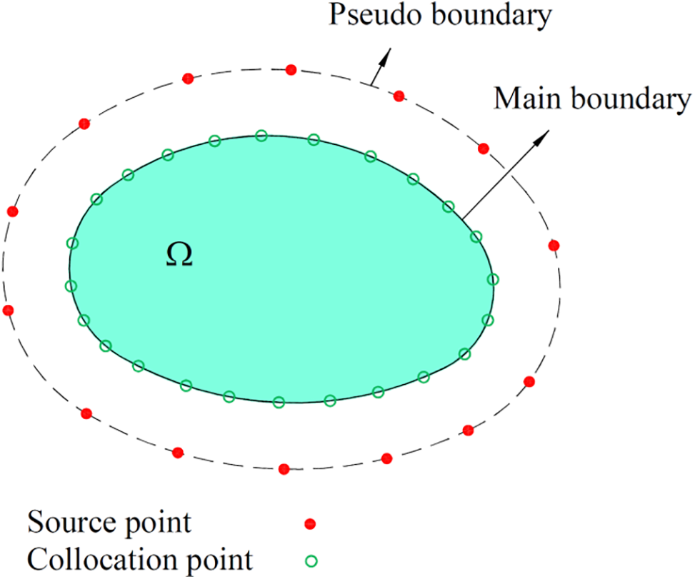
Figure 1: Source points and collocation points in the MFS

The components of the strain and stress tensors can be computed as follows:

εij(x)=∑k=1N[γk1εij1∗(x,Sk)+γk2εij2∗(x,Sk)],(8)

σij(x)=∑k=1N[γk1σij1∗(x,Sk)+γk2σij2∗(x,Sk)],(9)

εijm∗(x)=12[uim,j∗(x,Sk)+ujm,i∗(x,Sk)],(10)

{σ11k∗σ22k∗σ12k∗}=[a11a12a16a21a22a26a61a62a66]−1{ε11k∗ε22k∗2ε12k∗}.(11)

ui(x), εij(x), and σij(x) in Eqs. (7)–(9) satisfy the governing equations given in Eqs. (1) to (4). The boundary conditions given in Eqs. (5) and (6) are satisfied at M collocation points on the boundary of the problem, which leads to the following system of linear equations:

[A]⏟2M×2N{γ}⏟2N×1={f}⏟2M×1.(12)

M must be equal to or greater than N. In cases where M>N, Eq. (12) becomes an overdetermined system of equations, which can be solved using the least-squares method. Some remarks regarding the MFS for 2D anisotropic elasticity can be found in [45].

3  Inverse Analyses

The general schematic of the inverse problem for identifying the applied traction t on a part of the boundary of a 2D anisotropic medium is shown in Fig. 2. Boundary conditions on other parts of the boundary are known, and material properties are also assumed to be known. The values of the displacements or strains at NM measurement points are available. These measurement data are obtained from appropriate experiments in real applications; however, in this study, they are provided through numerical simulation by solving the corresponding direct problem using the MFS. The traction vector t is expressed in terms of m unknown parameters, i.e., f1,f2,…,fm, which must be found through the inverse analysis. For example, a quadratic variation with three parameters may be considered for the traction.

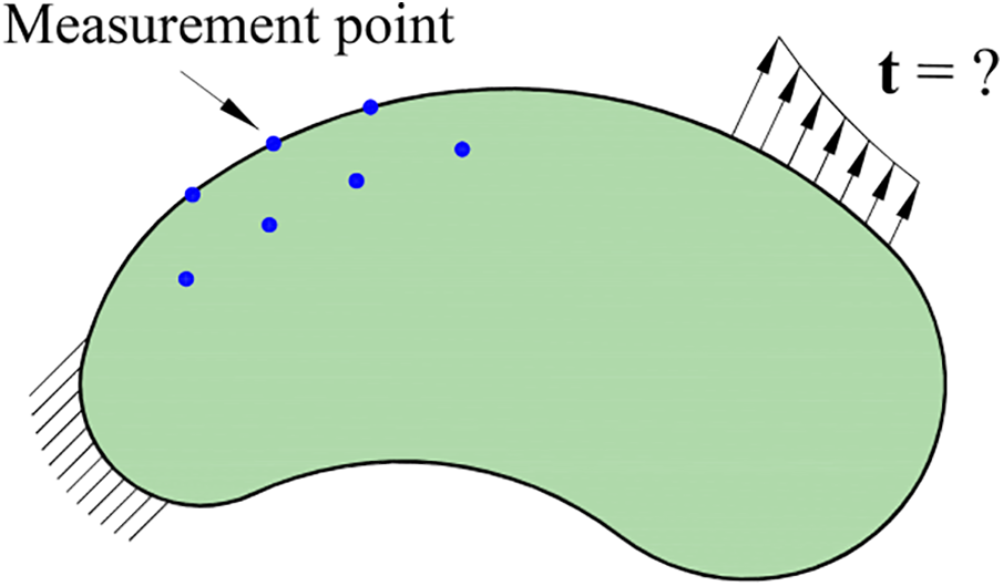
Figure 2: General schematic of the inverse problem for traction identification

The vector of unknowns is defined as follows:

{X}=[f1f2⋯fm]T.(13)

The vector of measurement data can be expressed as follows:

{Y¯}=[Y¯1Y¯2⋯Y¯NM]T.(14)

where Y¯i represents the displacement or strain measurement datum at the ith measurement point. Through the inverse analysis, the value of the displacement or strain at measurement points is reconstructed. The vector of the reconstructed parameters is expressed as follows:

{Y}=[Y1Y2⋯YNM]T.(15)

ϕ({X})=({Y}−{Y¯})T({Y}−{Y¯}).(16)

In cases where the ill-posedness of the inverse problem is considerable, such as when a small number of measurement data is available, the inverse solution for the components of {X} may be oscillatory. In these cases, the regularization term μR{X}T{X} can be added to the right-hand side of Eq. (16). μR is the regularization parameter and an appropriate value should be selected for it. Large values for μR result in a regularized solution, but the difference between measurement data and reconstructed measurement variables becomes large. On the other hand, if a very small value is selected for μR, the difference between {Y} and {Y¯} will be small, but the solution may be oscillatory. In this study, a quadratic form with three unknown parameters is considered for the traction and the oscillation of the solution is not significant; therefore, the inverse analysis is conducted without any regularization.

To minimize the cost function in Eq. (16), its derivative with respect to {X} is set equal to zero, yielding:

{S}T({Y}−{Y¯})=0,(17)

where {S} is the sensitivity matrix, the components of which are expressed as follows:

Sij=∂Yi∂Xji=1,2,…,NM,j=1,2,…,m.(18)

Since the problem is linear, one can substitute {Y}={S}{X} in Eq. (17), which results in:

{X}=({S}T{S})−1{S}T{Y¯}.(19)

To find the unknown vector {X} from Eq. (19), it is necessary to compute {S}. By solving m direct problems the components of {S} can be found. As the first problem in the sensitivity analysis, we set f1=1 and f2=f3=…=fm=0, and compute the measurement variables at the NM measurement points. Assuming that the computed values are Y1, Y2, ..., YNM, respectively, the first column of {S} can be set as Si1=Yi. Similarly by setting fj=1 and other traction parameters equal to zero and solving the direct problem the jth column of {S} is computed.

4  Numerical Study

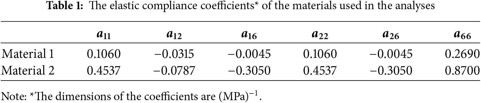
An inverse plane anisotropic problem in several different situations is presented in this section, and the influence of important parameters such as the number of measurement data, the location of measurement points, and the magnitude of the measurement error on the solution is investigated. Two different materials are considered in the analyses. The elastic compliance coefficients of these materials are given in Table 1.

A rectangular domain with a central hole is considered in the example. The geometry and boundary conditions of the direct problem are shown in Fig. 3. The left edge of the rectangle is fixed (i.e., ui=0), while the upper and lower edges, as well as the internal circular boundary, are traction free (i.e., σijnj=0), and the right edge of the rectangle (AB) is subjected to the normal traction t=f(y). Specifically, σ11 equals t, and the tangential component of the traction, σ12, is equall to zero on AB.

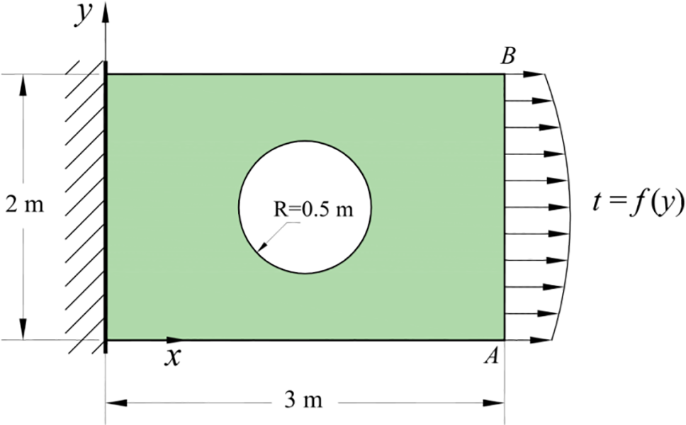
Figure 3: Geometry and boundary conditions of the problem

For constructing the inverse problems to be analyzed, three different functions are considered for the function f, which are given in Table 2. To provide the measurement data for the inverse analysis, the direct problem, subject to the three tractions on its right edge (i.e., AB) is solved, and the solutions for displacement and strain are found. The obtained solutions at some points, with added artificial errors, are used in the inverse analysis as the measurement data. Each measurement datum is simulated by adding a Gaussian error to the exact value as follows:

Y¯i=Y¯iexact+ei,(20)

where Y¯iexact is the exact value and Y¯i is the simulated value of the ith measured datum, and ei is the added error. ei corresponds to a noise level of T%  and is computed as follows:

ei=Y¯iexactγi(T/100),(21)

where γi is a random number with a Gaussian distribution in the interval [−1 1].

The geometry of the considered problem includes sharp corners and involves a curved boundary. Moreover, since the material is anisotropic and there are stress concentrations around the circle, the problem can be considered as a relatively complicated problem. A larger number of source points is required to solve anisotropic elastostatic problems than for isotropic problems [45]. The direct problem was solved three times using the MFS with 456, 912, and 1824 source points. The number of collocation points was considered to be two times the number of source points in each case. Through a numerical study it was observed that the case with 912 source points and 1824 collocation points results in a very accurate solution with less than 0.1% difference compared to the case with 1824 source points. Consequently, the model with 912 source points is used in the inverse analyses. The distance between the main and pseudo boundaries has been selected based on the procedure described in [45], where it is suggested to use the value of 0.95 for the location parameter of source points. Based on the procedure mentioned, the distance from the pseudo boundary to the main boundary is selected as 0.024 m and 0.1 m for the internal circle and the rectangle, respectively. Detailed explanations regarding the suitable distance between the main and pseudo boundaries for the analysis of 2D anisotropic elastostatic problems can be found in [45].

In the inverse analysis, the traction function on the edge AB is considered to be unknown. We approximate the traction with a quadratic function in terms of three unknown parameters as follows:

f=t1(y−1)(y−2)2+t2y(y−2)−1+t3y(y−1)2(22)

where t1, t2, and t3 in Eq. (22) are the unknown traction parameters. Indeed, t1, t2, and t3 represent the value of the traction on the edge AB at points with y=0, 1 and 2, respectively. The quadratic form considered for the unknown traction vector can exactly match the linear and quadratic functions given in Table 2; however, its form is different from the third case, which has a sinusoidal form. In the considered problem, the edge with unknown traction is straight. However, if the edge with the unknown condition is curved, the same procedure can be used since the unknown traction is expressed in terms of several unknown parameters, which can be found by inverse analysis.

The inverse analyses are performed with several different configurations of measurement points. Six different cases for the configuration of measurement points are shown in Fig. 4. There are 4 measurement points in Cases 1, 2, and 3 where the measurement points are closer to the edge AB in Case 1 and the distance from the measurement points to the edge AB is larger in Case 3. The number of measurement points has been increased to 8 and 12 in Cases 4 and 5, respectively. In Case 6, the measurement points are located on the boundary of the problem, where 6 measurement points have been considered.

Figure 4: Configuration of measurement points in the inverse analyses

The error percentage (based on the L2 norm) of the inverse solution is calculated by the following equation using the exact and computed values of the traction at 21 points on the edge AB:

Er=∑i=121(tiInv−tiExact)2∑i=121(tiExact)2×100%,(23)

where tiInv represents the magnitude of the traction at the ith point obtained by the inverse analysis and tiExact is the exact solution at the same point.

Now, the results obtained from different inverse analyses are reported. First, we study the accuracy of the inverse analysis with displacement and strain measurements. Strain at a point on the surface of a body can be simply measured by a strain gauge, while displacement measurement, especially when the magnitude of the displacement is small, may be more difficult. In Fig. 5, the results for the identification of the traction on edge AB in a case with Material 1 (Table 1), 3% measurement error, and with measurement points configuration of Case 1 (Fig. 4) are shown. At the first time, the displacement measurement data and at the second time the strain measurement data have been used. In Fig. 5a–c, the results for the traction with linear, quadratic, and sinusoidal variations (Table 2) are shown, respectively. As can be seen, the results obtained with strain measurements are clearly more accurate than the cases where displacement measurements are used. Therefore, in the next inverse analyses, strain measurements are used for the identification of the traction.

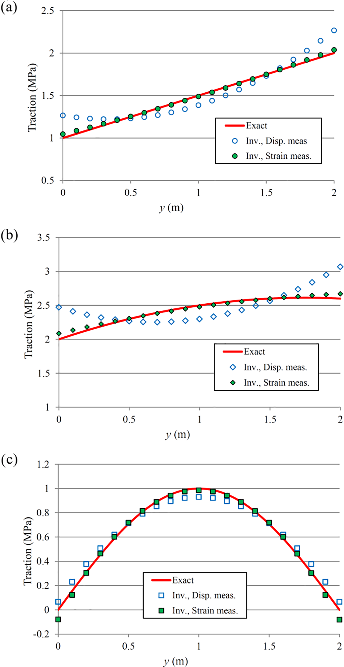
Figure 5: Results of the inverse analysis for the traction identification with Material 1, Case 1 of measurement points configuration, 3% measurement error, and with displacement and strain measurements: (a) linear traction, (b) quadratic traction, (c) sinusoidal traction

In Fig. 6, the results for the identification of the traction on edge AB in a case with Material 1 (Table 1), with 0%, 5% and 10% measurement error (strain measurement), and with measurement points configuration of Case 2 (Fig. 4) are shown. In Fig. 6a–c, the results for the traction with linear, quadratic, and sinusoidal variations (Table 2) are shown, respectively. When the measurement error is zero, the tractions with linear and quadratic forms are identified without any error. However, there is an error of 3.5% in the identification of the traction with sinusoidal variation. The magnitude of the error is computed using Eq. (23). In the case with 5% measurement error, the error of the identified traction is 3.0%, 3.5%, and 3.6% for linear, quadratic, and sinusoidal tractions, respectively. In the case with 10% measurement error, which is a significantly large magnitude, the error of the identified traction is 6.0%, 7.0%, and 6.7% for linear, quadratic and sinusoidal tractions, respectively. From the results shown in Fig. 6 it is observed that the inverse method is capable of traction identification even with considerable measurement error. Moreover, it is seen that the method can identify a traction with a different form than the one considered for the traction in the inverse analysis.

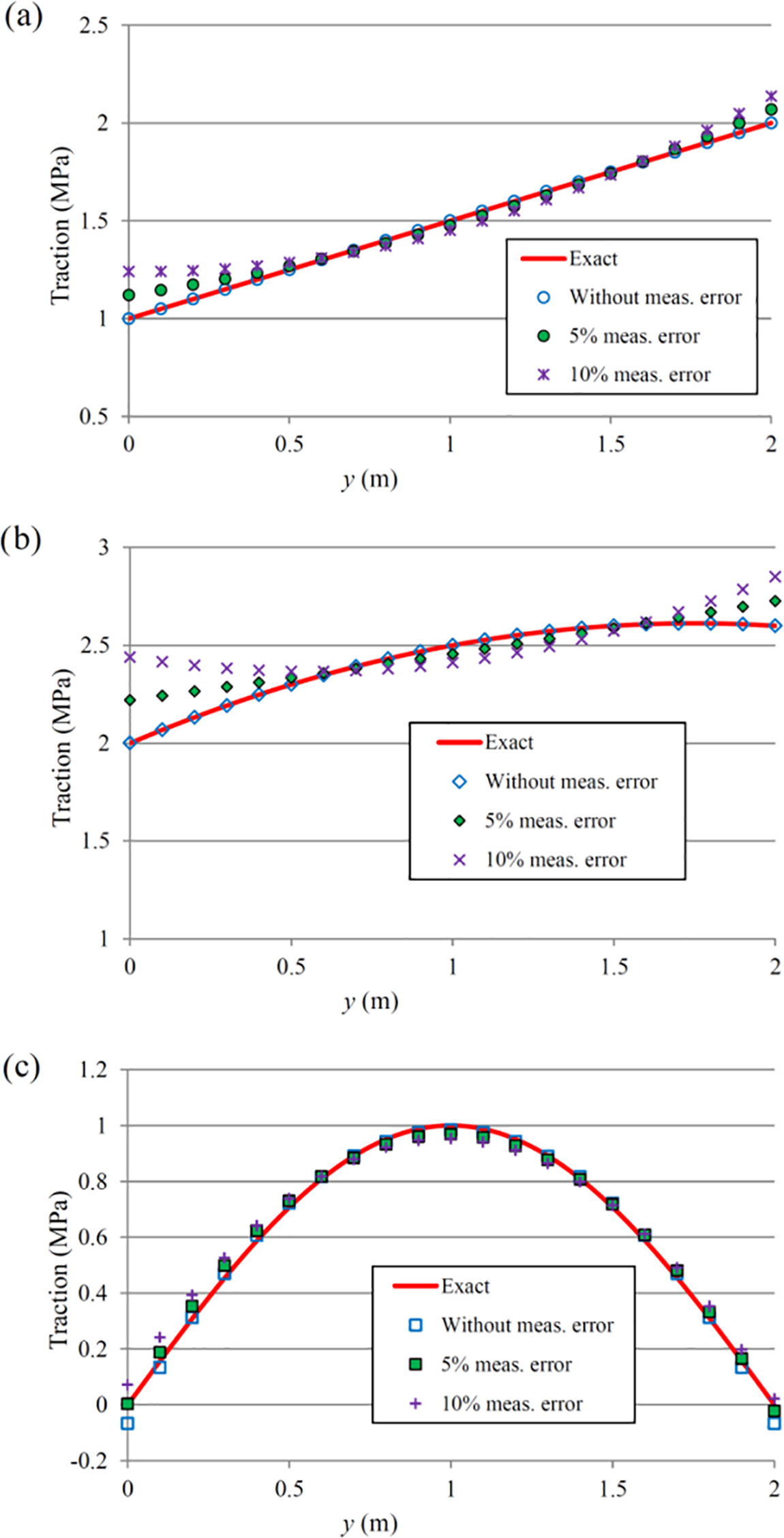
Figure 6: Results of the inverse analysis for the traction identification with Material 1, different measurement errors and Case 2 of configurations of measurement points: (a) linear traction, (b) quadratic traction, (c) sinusoidal traction

In the next inverse analysis, we study the influence of the location of the measurement points on the accuracy of the identified traction. The results of the inverse analysis for the traction identification with 3% measurement error, Material 1, and two different configurations of measurement points are shown in Fig. 7. In the first analysis, the 4 measurement points of Case 1 (in Fig. 4) are used in the inverse analysis. In the next analysis, the 4 measurement points of Case 3 are used in the inverse analysis. In Case 1, the measurement points are close to the edge with unknown traction (edge AB), while the measurement points are relatively far from edge AB in Case 3. From Fig. 7, it is observed that the obtained results are much more accurate when the measurement points are close to the edge with unknown traction.

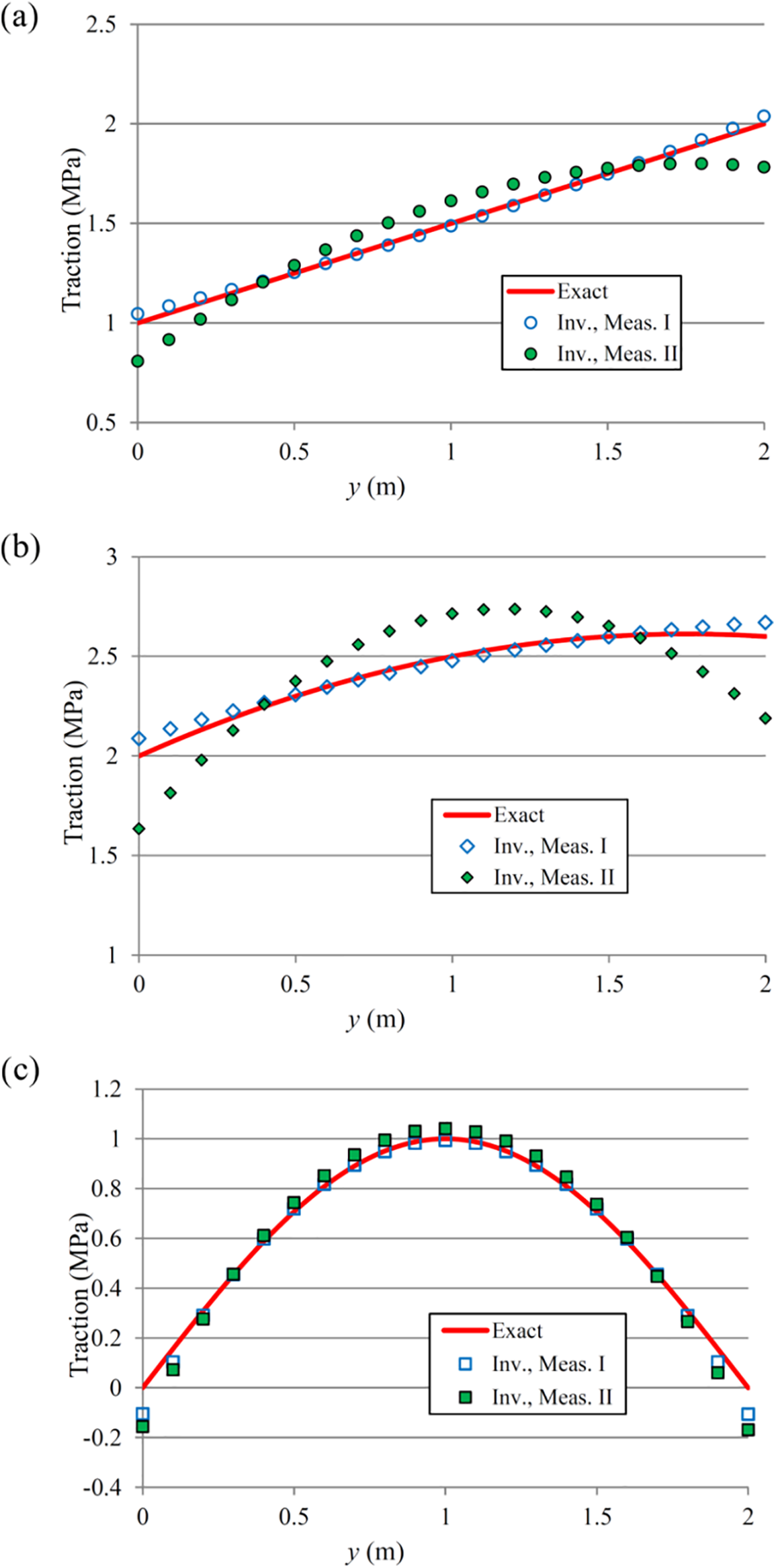
Figure 7: Results of the inverse analysis for the traction identification with 3% measurement error, Material 1, and two different configurations of measurement points: (a) linear traction, (b) quadratic traction, (c) sinusoidal traction, “Inv., Meas. I” and “Inv. Meas. II” in the legends correspond to measurement points configurations 1 and 3 in Fig. 4, respectively

The influence of the number of measurement data on the accuracy of the identified traction is also studied. The results of the inverse analysis for the traction identification with 10% measurement error, Material 1, and with 4, 8 and 12 measurement points are shown in Fig. 8. Cases 1, 4, and 5 in Fig. 4 correspond to the three cases with 4, 8, and 12 measurement points, respectively. As can be seen from Fig. 8, by increasing the number of measurement points from 4 to 8, the accuracy of the results is significantly increased. Further increase of the measurement points from 8 to 12 has no significant effect on increasing the accuracy of the results. In other words, when the number of measurement points is not large, increasing the number of measurement points will increase the accuracy of the inverse solution; however, in cases with a large number of measurement points, further increase of the number of measurement data has little effect on the results.

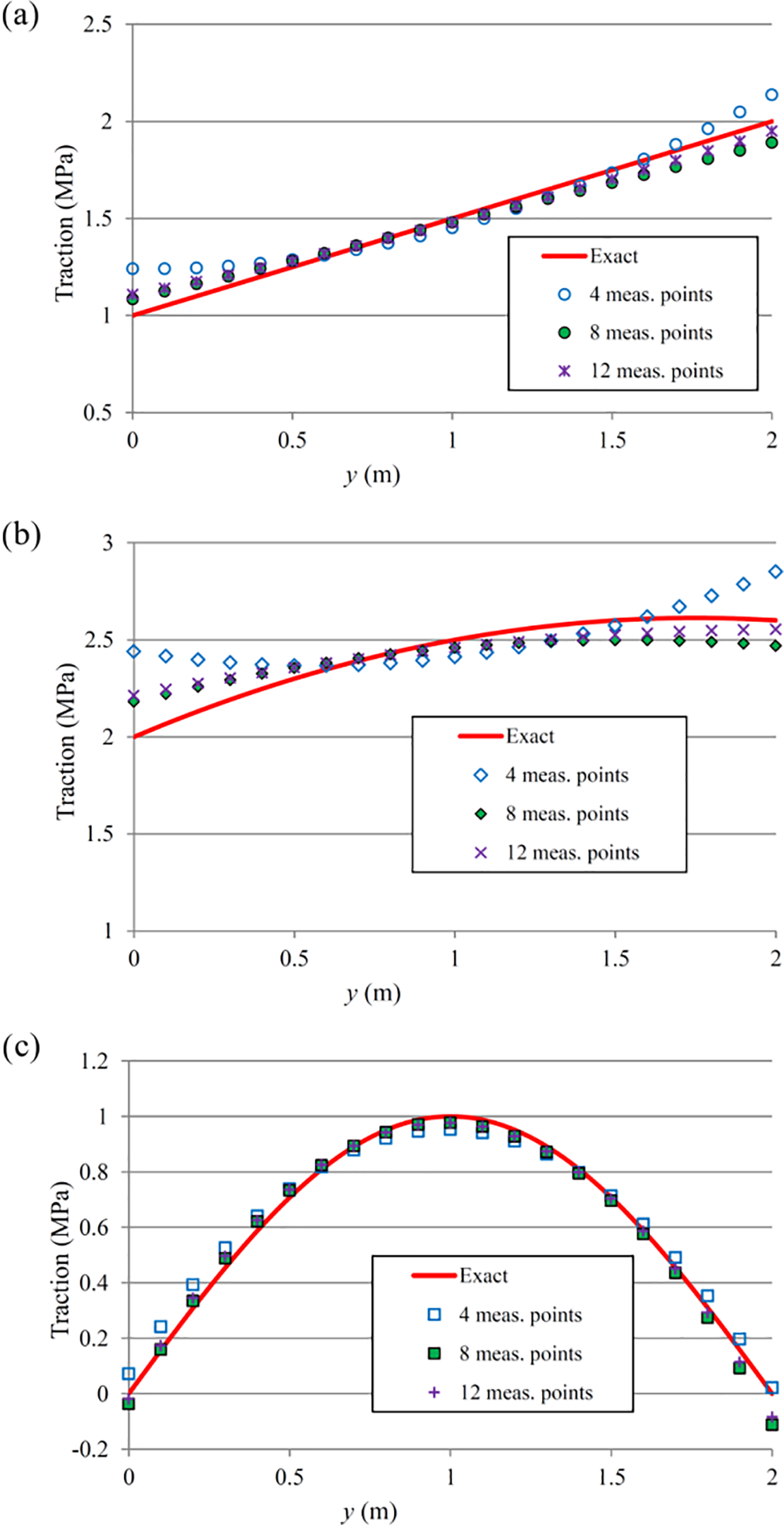
Figure 8: Results of the inverse analysis for the traction identification with 10% measurement error, Material 1, and with 4, 8 and 12 measurement points: (a) linear traction, (b) quadratic traction, (c) sinusoidal traction

In all of the previous inverse analyses, the measurement points were located within the domain of the problem. A case with measurement points on the boundary is also considered. The results for this case with Material 1, with 0%, 5%, and 10% measurement error, and with 6 measurement points (Case 6 in Fig. 4) are shown in Fig. 9. As can be seen from Fig. 9, the inverse method can efficiently identify the unknown traction using measurement points located on the boundary.

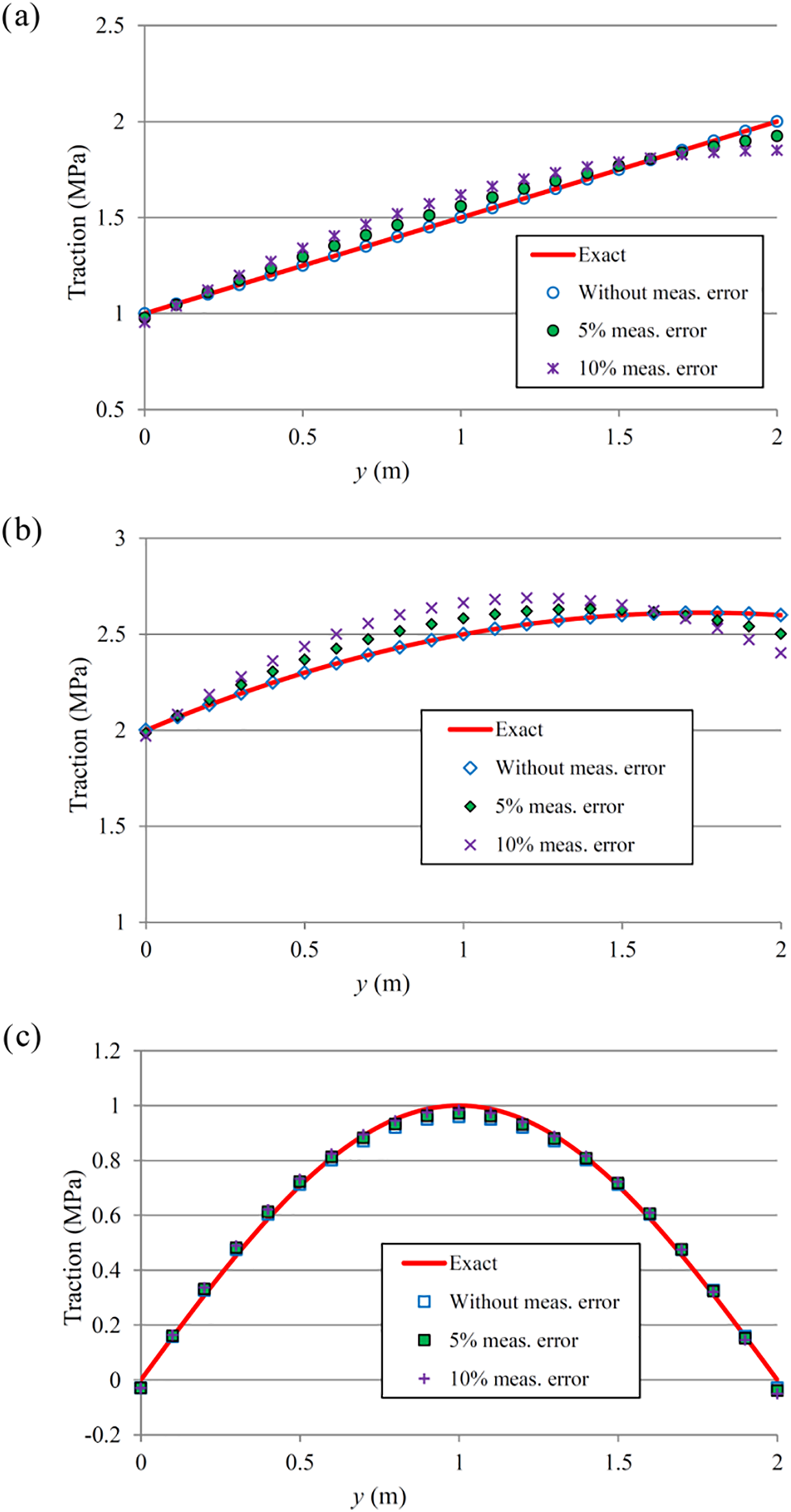
Figure 9: Results of the inverse analysis for the traction identification with 0%, 5%, and 10% measurement error, Material 1, and with 6 measurement points on the boundary: (a) linear traction, (b) quadratic traction, (c) sinusoidal traction

In all of the previous analyses, Material 1 was used. To ensure that the inverse method is capable of finding acceptable solutions for different materials, another analysis with Material 2 (Table 1) is also performed. The results for this case with Material 2, with 0%, 5%, and 10% measurement error, and with 4 measurement points (Case 2 in Fig. 4) are shown in Fig. 10. This figure shows that the inverse method can identify the unknown traction with sufficient accuracy for the case with Material 2 as well. It should be mentioned that the inverse method proposed in this study is applicable to problems with linear anisotropic materials. For more advanced anisotropic materials with large deformations [48], a different method should be developed.

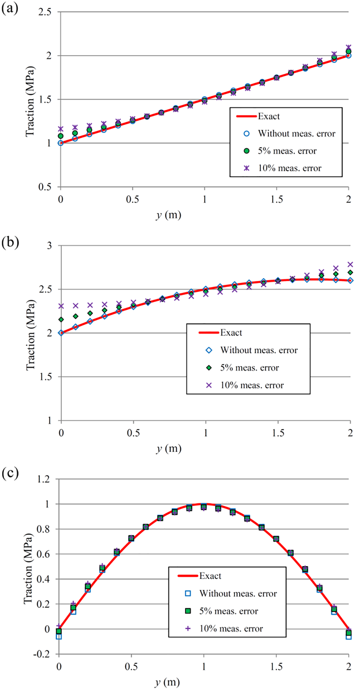
Figure 10: Results of the inverse analysis for the traction identification with 0%, 5%, and 10% measurement error, Material 2, and with 4 measurement point: (a) linear traction, (b) quadratic traction, (c) sinusoidal traction

5  Conclusions and Remarks

The MFS is computationally efficient. Moreover, boundary conditions are applied in a strong form in this method. Consequently, the MFS can be effectively utilized to identify an unknown traction along a part of the surface of a solid. An inverse MFS based on displacement and strain measurements was presented to identify traction on a part of the boundary of an anisotropic domain. Several inverse analyses were performed to determine various traction forces on the edge of an anisotropic body. The key conclusions drawn from this research are summarized as follows:

–   Some inverse analyses based on displacement and strain measurements were performed, and it was observed that the results obtained using strain measurements were more accurate than those obtained using displacement measurements. This can be explained by the fact that the displacement field includes both deformation and rigid-body motion, while the strain field reflects only the deformation, which is more sensitive to the applied traction.

–   The results indicated that the proposed inverse method is capable of identifying traction even in cases with significant measurement error. It was also observed that the method can identify traction in a form different from the one considered for the unknown traction in the inverse analysis.

–   The solution of the inverse method is more accurate when the measurement points are closer to the edge with the unknown traction. As the distance from the measurement points to the edge increases, the sensitivity of the structural response at those points to the traction parameters decreases. Consequently, the ill-posedness of the inverse problem increases, which leads to a decrease in the accuracy of the solution.

–   In cases where the number of measurement points is small, increasing the number of measurement points significantly enhances the accuracy of the inverse solution. However, when there are a sufficient number of measurement points, further increases have little effect on the results. In this work, each test problem involved 3 unknowns, and it was observed that using 4 to 8 measurement points yields sufficiently accurate solutions.

–   The inverse analysis conducted in this study revealed that the proposed method can efficiently identify unknown traction using measurement points located along the boundary. Furthermore, the method demonstrated insensitivity to material properties. Examples involving two different anisotropic materials showed that the solutions obtained in both cases were sufficiently accurate.

–   In this study, a continuous form was considered for the unknown traction function. If the actual applied traction is discontinuous, the inverse method will identify a continuous function that reconstructs the measurement data as accurately as possible. It should also be noted that for cases with a highly complex or discontinuous traction function, incorporating a greater number of parameters in the function used to represent the unknown traction will enhance the solution of the inverse problem.

–   It should be noted that the MFS and the inverse method developed in this study are applicable to problems involving linear anisotropic materials. For more advanced nonlinear anisotropic materials, a different method should be developed.

Acknowledgment: Not applicable.

Funding Statement: This research was funded by Vice Chancellor of Research at Shiraz University (grant 3GFU2M1820).

Availability of Data and Materials: The data that support the findings of this study are available from the author upon reasonable request.

Ethics Approval: Not applicable.

Conflicts of Interest: The author declares no conflicts of interest to report regarding the present study.

Appendix A Displacement Fundamental Solutions

In this appendix, the displacement fundamental solution for anisotropic elasticity in 2D is described. We denote the displacement fundamental solution as uij∗(x,S), where the source point S has coordinates (x0,y0) and the field point x has coordinates (x,y). The fundamental solution can be expressed as follows [46,47]:

uij∗(x,S)=2Re[Pi1Aj1ln⁡(z1−z01)+Pi2Aj2ln⁡(z2−z02)].(A1)

z1, z2, z01, and z02 in Eq. (A1) are expressed as follows:

z1=x+μ1y,z2=x+μ2y,(A2)

z01=x0+μ1y0,z02=x0+μ2y0,(A3)

a11μ4−2a16μ3+(2a12+a66)μ2−2a26μ+a22=0.(A4)

This equation has four complex roots. The imaginary parts of two roots (μ1 and μ2) are positive, while the imaginary parts of the other roots are negative. Pik in Eq. (A1) are determined as follows:

P1k=a11μk2+a12−a16μk,P2k=a12μk+a22/μk−a26,k=1,2.(A5)

Aji are also complex numbers. The real and imaginary parts (i.e., Re( ) and Im( )) of Aji can be determined by solving the following matrix equation:

[0101Im(μ1)Re(μ1)Im(μ2)Re(μ2)Im(P11)Re(P11)Im(P12)Re(P12)Im(P21)Re(P21)Im(P22)Re(P22)][Re(Ai1)Im(Ai1)Re(Ai2)Im(Ai2)]=[−δi2/4πδi1/4π00],i=1,2.(A6)

where δij denotes the Kronecker delta. In the MFS formulation, it is required to find the derivatives of uij∗, which can be found using the following equation:

uij,k∗=2Re[Pi1Aj1Tk1(z1−z01)+Pi2Aj2Tk2(z2−z02)],(A7)

where T11, T12, T21, and T22 are equal to 1, 1, μ1, and μ2, respectively.

References

1. Groetsch CW. Inverse problems in the mathematical sciences. Braunschweig: Vieweg; 1993. [Google Scholar]

2. Van Hemelrijck D, Makris A, Ramault C, Lamkanfi E, Van Paepegem W, Lecompte D. Biaxial testing of fibre-reinforced composite laminates. Proc Inst Mech Eng Pt L J Mater Des Appl. 2008 Oct 1;222(4):231–9. doi:10.1243/14644207JMDA199. [Google Scholar] [PubMed] [CrossRef]

3. Hematiyan MR, Khosravifard A, Shiah YC, Tan CL. Identification of material parameters of two-dimensional anisotropic bodies using an inverse multi-loading boundary element technique. Comput Model Eng Sci. 2012 Sep 1;87(1):55–76. doi:10.3970/cmes.2012.087.055. [Google Scholar] [CrossRef]

4. Nigamaa N, Subramanian SJ. Identification of orthotropic elastic constants using the eigenfunction virtual fields method. Int J Solids Struct. 2014 Jan 15;51(2):295–304. doi:10.1016/j.ijsolstr.2013.09.021. [Google Scholar] [CrossRef]

5. Chen B, Chen W, Wei X. Identification of elastic orthotropic material parameters by the singular boundary method. Adv Appl Math Mech. 2016 Oct;8(5):810–26. doi:10.4208/aamm.2015.m904. [Google Scholar] [CrossRef]

6. Hematiyan MR, Khosravifard A, Shiah YC. A new stable inverse method for identification of the elastic constants of a three-dimensional generally anisotropic solid. Int J Solids Struct. 2017 Feb 1;106:240–50. doi:10.1016/j.ijsolstr.2016.11.009. [Google Scholar] [CrossRef]

7. Smyl D, Antin KN, Liu D, Bossuyt S. Coupled digital image correlation and quasi-static elasticity imaging of inhomogeneous orthotropic composite structures. Inverse Prob. 2018;34(12):124005. doi:10.1088/1361-6420/aae793. [Google Scholar] [CrossRef]

8. Mei Y, Goenezen S. Quantifying the anisotropic linear elastic behavior of solids. Int J Mech Sci. 2019;163:105131. doi:10.1016/j.ijmecsci.2019.105131. [Google Scholar] [CrossRef]

9. Kim C, Kim JH, Lee MG. A virtual fields method for identifying anisotropic elastic constants of fiber reinforced composites using a single tension test: theory and validation. Compos B Eng. 2020 Nov 1;200:108338. [Google Scholar]

10. Zhang W, Alkhazaleh HA, Samavatian M, Samavatian V. Machine learning-assisted investigation of anisotropic elasticity in metallic alloys. Mater Today Commun. 2024;40:109950. doi:10.1016/j.mtcomm.2024.109950. [Google Scholar] [CrossRef]

11. Hematiyan MR, Khosravifard A, Mohammadi M, Shiah YC. An inverse method of fundamental solutions for the identification of 2D elastic properties of anisotropic solids. J Braz Soc Mech Sci Eng. 2024 Jun;46(6):357. [Google Scholar]

12. Bilotta A, Turco E. A numerical study on the solution of the Cauchy problem in elasticity. Int J Solids Struct. 2009 Dec 15;46(25–26):4451–77. [Google Scholar]

13. Durand B, Delvare F, Bailly P. Numerical solution of Cauchy problems in linear elasticity in axisymmetric situations. Int J Solids Struct. 2011 Oct 15;48(21):3041–53. [Google Scholar]

14. Zhou H, Jiang W, Hu H, Niu Z. Boundary element methods for boundary condition inverse problems in elasticity using PCGM and CGM regularization. Eng Anal Bound Elem. 2013 Nov 1;37(11):1471–82. [Google Scholar]

15. Li PW, Fu ZJ, Gu Y, Song L. The generalized finite difference method for the inverse Cauchy problem in two-dimensional isotropic linear elasticity. Int J Solids Struct. 2019 Nov 10;174:69–84. [Google Scholar]

16. Mei Y, Zhao D, Kang R, Wang X, Wang B, Song D, et al. Non-contact reconstitution of the traction distribution using incomplete deformation measurements: methodology and experimental validation. Int J Solids Struct. 2024 Mar 1;289:112650. [Google Scholar]

17. Comino L, Marin L, Gallego R. An alternating iterative algorithm for the Cauchy problem in anisotropic elasticity. Eng Anal Bound Elem. 2007 Aug 1;31(8):667–82. doi:10.1016/j.enganabound.2006.12.009. [Google Scholar] [CrossRef]

18. Zhang T, Dong L, Alotaibi A, Atluri SN. Application of the MLPG mixed collocation method for solving inverse problems of linear isotropic/anisotropic elasticity with simply/multiply-connected domains. Comput Model Eng Sci. 2013 Jul 1;94(1):1–28. [Google Scholar]

19. Zhang T, Dong L, Alotaibi A, Atluri SN. Application of the Trefftz method, on the basis of Stroh formalism, to solve the inverse Cauchy problems of anisotropic elasticity in multiply connected domains. Eng Anal Bound Elem. 2014 Jun 1;43(3):95–104. doi:10.1016/j.enganabound.2014.03.012. [Google Scholar] [CrossRef]

20. Karageorghis A, Lesnic D, Marin L. A survey of applications of the MFS to inverse problems. Inverse Prob Sci Eng. 2011 Jan 1;19(3):309–36. doi:10.1080/17415977.2011.551830. [Google Scholar] [CrossRef]

21. Marin L. Reconstruction of boundary data in two-dimensional isotropic linear elasticity from Cauchy data using an iterative MFS algorithm. Comput Model Eng Sci. 2010 May 1;60(3):221–46. doi:10.3970/cmes.2010.060.221. [Google Scholar] [CrossRef]

22. Marin L, Delvare F, Cimetière A. Fading regularization MFS algorithm for inverse boundary value problems in two-dimensional linear elasticity. Int J Solids Struct. 2016 Jan 1;78:9–20. [Google Scholar]

23. Marin L, Cipu C. Non-iterative regularized MFS solution of inverse boundary value problems in linear elasticity: a numerical study. Appl Math Comput. 2017 Jan 15;293:265–86. [Google Scholar]

24. Mathon R, Johnston RL. The approximate solution of elliptic boundary-value problems by fundamental solutions. SIAM J Num Anal. 1977 Sep;14(4):638–50. [Google Scholar]

25. Cheng AH, Hong Y. An overview of the method of fundamental solutions—Solvability, uniqueness, convergence, and stability. Eng Anal Bound Elem. 2020 Nov 1;120:118–52. [Google Scholar]

26. Golberg MA. The method of fundamental solutions for Poisson’s equation. Eng Anal Bound Elem. 1995 Oct 1;16(3):205–13. [Google Scholar]

27. Fairweather G, Karageorghis A. The method of fundamental solutions for elliptic boundary value problems. Adv Comput Math. 1998 Sep;9:69–95. doi:10.1023/A:1018981221740. [Google Scholar] [CrossRef]

28. Redekop D. Fundamental solutions for the collation method in planar elastostatics. Appl Math Model. 1982 Oct 1;6(5):390–3. doi:10.1016/S0307-904X(82)80104-2. [Google Scholar] [CrossRef]

29. Berger JR, Karageorghis A. The method of fundamental solutions for layered elastic materials. Eng Anal Bound Elem. 2001 Dec 1;25(10):877–86. doi:10.1016/S0955-7997(01)00002-9. [Google Scholar] [CrossRef]

30. Tsai CC. The method of fundamental solutions with dual reciprocity for three-dimensional thermoelasticity under arbitrary body forces. Eng Comput. 2009;26(3):229–44. doi:10.1108/02644400910943590. [Google Scholar] [CrossRef]

31. Marin L, Karageorghis A. The MFS-MPS for two-dimensional steady-state thermoelasticity problems. Eng Anal Bound Elem. 2013 Jul 1;37(7–8):1004–20. doi:10.1016/j.enganabound.2013.04.002. [Google Scholar] [CrossRef]

32. Hematiyan MR, Mohammadi M, Tsai CC. The method of fundamental solutions for anisotropic thermoelastic problems. Appl Math Model. 2021 Jul 1;95(9):200–18. doi:10.1016/j.apm.2021.02.001. [Google Scholar] [CrossRef]

33. Kondapalli PS, Shippy DJ, Fairweather G. The method of fundamental solutions for transmission and scattering of elastic waves. Comput Methods Appl Mech Eng. 1992 Apr 1;96(2):255–69. doi:10.1016/0045-7825(92)90135-7. [Google Scholar] [CrossRef]

34. Khoshroo M, Hematiyan MR, Daneshbod Y. Two-dimensional elastodynamic and free vibration analysis by the method of fundamental solutions. Eng Anal Bound Elem. 2020 Aug 1;117(10):188–201. doi:10.1016/j.enganabound.2020.04.014. [Google Scholar] [CrossRef]

35. Wen PH, Adetoro M, Xu Y. The fundamental solution of Mindlin plates with damping in the Laplace domain and its applications. Eng Anal Bound Elem. 2008 Oct 1;32(10):870–82. doi:10.1016/j.enganabound.2007.12.005. [Google Scholar] [CrossRef]

36. Tsiatas GC. A new Kirchhoff plate model based on a modified couple stress theory. Int J Solids Struct. 2009 Jun 15;46(13):2757–64. doi:10.1016/j.ijsolstr.2009.03.004. [Google Scholar] [CrossRef]

37. Lei B, Fan CM, Li M. The method of fundamental solutions for solving non-linear Berger equation of thin elastic plate. Eng Anal Bound Elem. 2018 May 1;90:100–6. doi:10.1016/j.enganabound.2018.02.007. [Google Scholar] [CrossRef]

38. Sun L, Fu Z, Chen Z. A localized collocation solver based on fundamental solutions for 3D time harmonic elastic wave propagation analysis. Appl Math Comput. 2023;439:127600. doi:10.1016/j.amc.2022.127600. [Google Scholar] [CrossRef]

39. Sun L, Ji Z, Zhang Q, Wei X. A localized meshless collocation method based on fundamental solutions for 3D uncoupled transient thermoelastic problems. Int J Heat Mass Transf. 2024;232(4):125945. doi:10.1016/j.ijheatmasstransfer.2024.125945. [Google Scholar] [CrossRef]

40. Xia H, Gu Y. The generalized finite difference method for electroelastic analysis of 2D piezoelectric structures. Eng Anal Bound Elem. 2021;124(2):82–6. doi:10.1016/j.enganabound.2020.12.012. [Google Scholar] [CrossRef]

41. Liu T, Wei G, Zhang Y. Radial basis reproducing kernel particle method for damped elastic dynamics problems. Iran J Sci Technol Trans Mech Eng. 2024;48(3):1161–76. doi:10.1007/s40997-023-00701-6. [Google Scholar] [CrossRef]

42. Hsiao YF, Shiah YC. Efficient BEM modeling of the heat transfer in the turbine blades of aero-parts. Aerospace. 2023;10(10):885. doi:10.3390/aerospace10100885. [Google Scholar] [CrossRef]

43. Akay AA, Gürses E, Göktepe S. A non-iterative boundary element formulation for nonlinear viscoelasticity. Eng Anal Bound Elem. 2024;163(12):223–36. doi:10.1016/j.enganabound.2024.03.010. [Google Scholar] [CrossRef]

44. Sadd MH. Elasticity: theory, applications, and numerics. Burlington, MA, USA: Academic Press; 2009 Feb 25. [Google Scholar]

45. Hematiyan MR, Jamshidi B, Mohammadi M. The method of fundamental solutions for two-dimensional elastostatic problems with stress concentration and highly anisotropic materials. Comput Model Eng Sci. 2022 Mar 1;130(3):1349–69. doi:10.32604/cmes.2022.018235. [Google Scholar] [CrossRef]

46. Lekhnitŝkiĭ SG. Theory of elasticity of an anisotropic elastic body. San Francisco: Holden-Day; 1963. [Google Scholar]

47. Cruse TA. Boundary element analysis in computational fracture mechanics. Dordrecht, Netherlands: Kluwer Academic Publishers; 1988. [Google Scholar]

48. Wollner MP, Terzano M, Rolf-Pissarczyk M, Holzapfel GA. A general model for anisotropic pseudo-elasticity and viscoelasticity at finite strains. J Mech Phys Solids. 2023;180(10):105403. doi:10.1016/j.jmps.2023.105403. [Google Scholar] [CrossRef]