
 Submit a Paper
 Propose a Special lssue
 Open Access
REVIEW

A Review of the Numerical Methods for Diblock Copolymer Melts
Department of Mathematics, Korea University, Seoul, 02841, Republic of Korea
* Corresponding Author: Junseok Kim. Email:
Computers, Materials & Continua 2025, 82(2), 1811-1838. https://doi.org/10.32604/cmc.2025.061071
Received 16 November 2024; Accepted 20 January 2025; Issue published 17 February 2025
 View Full Text
 Download PDF
Abstract
This review paper provides a comprehensive introduction to various numerical methods for the phase-field model used to simulate the phase separation dynamics of diblock copolymer melts. Diblock copolymer systems form complex structures at the nanometer scale and play a significant role in various applications. The phase-field model, in particular, is essential for describing the formation and evolution of these structures and is widely used as a tool to effectively predict the movement of phase boundaries and the distribution of phases over time. In this paper, we discuss the principles and implementations of various numerical methodologies for this model and analyze the strengths, limitations, stability, accuracy, and computational efficiency of each method. Traditional approaches such as Fourier spectral methods, finite difference methods and alternating direction explicit methods are reviewed, as well as recent advancements such as the invariant energy quadratization method and the scalar auxiliary variable scheme are also presented. In addition, we introduce examples of the phase-field model, which are fingerprint image restoration and 3D printing. These examples demonstrate the extensive applicability of the reviewed methods and models.Keywords
In this review, we present an overview of the numerical methodologies for diblock copolymer melts. The Ohta–Kawasaki equation, introduced by Ohta et al. [1], was originally developed to explain the microphase separation patterns in diblock copolymer melts. A diblock copolymer is defined as a polymer composed of two distinct subchains linked by a covalent bond, with each subchain composed of monomers that repel each other. When a large number of such molecules aggregate, they form a structure known as a melt. These diblock copolymer melts are of great interest in both scientific and engineering fields due to their unique phase separation behavior. Their distinct constituent monomers separate to form nanoscale structures with desirable properties [2]. This phase separation is a process known as spinodal decomposition, which enables the formation of various microstructures such as lamellar, cubic, hexagonal, and gyroid configurations depending on the synthetic conditions used [3]. These diverse structures can significantly influence the mechanical properties of the material [4], and it is therefore essential to anticipate the structure that will be formed experimentally.
Due to these unique characteristics, diblock copolymer melts have found applications across multiple fields, such as materials science [5,6], nanotechnology [7–9], and biomedical engineering [10]. Controlled pattern formation at the nanoscale can improve the mechanical, optical, and electrical properties of materials, and enable the creation of advanced materials tailored for specific functions [11]. Several computational algorithms have been proposed to analyze the equilibrium state of diblock copolymers. Techniques such as Monte Carlo methods [12–14], molecular dynamics [15], self-consistent field theory [16,17], cell dynamics simulations [18], dissipative particle dynamics simulations [19–21] and the phase-field model [22–24] are widely used for this purpose. The phase-field model, in particular, is a continuum model that describes the interface using the order parameter. This model is advantageous because it bypasses the need to solve complex boundary value problems, as it formulates the governing equations through the variation of an energy functional. Consequently, the phase-field model has become a widely adopted approach for reproducing various material structures, and it enables researchers to derive the governing equations in a relatively straightforward manner [25–27]. Researchers also constructed new or modified phase field equations for the diblock copolymer solutions for specific conditions and cases. Shen et al. [28] proposed a thermodynamically consistent phase field equation for the simulation of diblock copolymers. The electric and magnetic field is coupled in the proposed model. The authors constructed the phase field model based on the Onsager principle. In order to solve the proposed model, the energy quadratization technique is applied, while the thermodynamical consistency is preserved. Numerical simulations showed convergence rate of the proposed algorithm and the effects of electric fields and magnetic field on the diblock copolymer system.
The Cahn–Hilliard (CH) equation is a fundamental governing equation in phase-field models and is widely used to describe phase separation phenomena in binary systems. It effectively models the evolution of the compositional concentration field and reveals the role of interface thickness in structure dynamics. The Navier–Stokes equations can model the flow of phases, and various numerical methods have been developed for their solutions [29]. When coupled with the CH equation, the Navier–Stokes equations can be used to model the flow of polymer melts. Song et al. [30] introduced an innovative, unconditionally energy-stable data assimilation algorithm for solving the Navier–Stokes–Cahn–Hilliard equations. Their approach demonstrated robust performance in handling locally discrete observational data. Song et al. [31] proposed an unconditionally energy-stable numerical method for the CH equation and validated its efficiency and stability through numerical experiments involving complex initial conditions. The CH equation is frequently coupled with other equations to capture additional characteristics. Martínez–Agustín et al. [32] proposed coupling the CH equation with the Swift–Hohenberg equation in 3D to model phase transitions in diblock copolymers. The proposed method is solved using the fast Fourier transform and a pseudo-spectral implicit method. Since the model dynamics can produce various morphologies, the porous polymeric materials obtained from numerical simulations have potential applications in 3D printing. As the Ohta–Kawasaki model explains the microphase separation patterns in diblock copolymer melts, Barua et al. [33] rescaled the Ohta–Kawasaki model, free energy, and boundary conditions for more efficient calculations of sharp-interfacial symmetric diblock copolymer problem. They applied boundary integral formulation and small-scale decomposition to solve the governing equations numerically. Their simulations illustrate the evolution of the system from the initial to intermediate states and eventually to the steady. Meng et al. [34] proposed a solution for the nonlocal CH equation with a nonlocal diffusion operator by using a scalar auxiliary variable method. Their proposed methods are unconditionally stable and showed high-order accuracy. Numerical solutions were efficiently obtained using the fast Fourier transform and gradient approach to achieve low storage cost and calculation time. The nonlocal CH equation with degenerate mobility was studied by Elbar et al. [35], where the additional nonlocal term accounts for the surface tension to model long-range interactions.
The Ohta–Kawasaki model, defined on the domain
where
where G is a Green’s function [36]. We can rewrite the long-range energy by considering the periodic or zero Neumann boundary conditions.
where
We also obtain the following energy dissipation law and mass conservation property [37].
and
where the integral by parts and periodic or zero Neumann boundary conditions are applied. Therefore, the Ohta–Kawasaki model satisfies the energy dissipation law and mass conservation by Eqs. (7) and (8), respectively. Because of these two fundamental properties of the Ohta–Kawasaki model, it is natural and important to construct proper numerical schemes that still satisfy these two properties in discrete manners. Singh et al. [9] developed a thermodynamically consistent nonlocal model for phase transformation and heat transfer in block copolymer directed self-assembly using the continuum theory of mixtures. Their model incorporates mass and energy balances, microforce balances, and constitutive relations to couple the phase field and temperature.They developed a finite element solution incorporating stable time-stepping schemes and performed computational tests to validate the equation’s effectiveness in simulating the self-assembly behavior of block copolymers. Chen et al. [38] proposed an efficient leapfrog time-marching method for the phase-field diblock copolymer equation, which significantly reduces the computational cost by requiring only the solution of a linear algebra system at each time step, ensures unconditional energy stability for large time steps, and guarantees the existence and uniqueness of the computational solution at each step, ensuring both reliability and accuracy. This method consists of the leapfrog integration scheme for time discretization and the Fourier spectral method for spatial discretization. The authors analyze the energy dissipation and mass conservation of the proposed numerical method for the Ohta–Kawasaki model and prove that the numerical scheme satisfies both properties. Li et al. [39] developed a highly efficient computational method for a flow-coupled phase-field equation for diblock copolymer melts. This model represents a complex nonlinear system consisting of the Navier–Stokes equations coupled with the CH type equation with an Ohta–Kawasaki potential. By combining decoupling techniques with the projection method, the authors developed a fully decoupled, energy-stable, second-order time-accurate computational method for the model. The decoupling technique is based on designing an auxiliary ordinary differential equation (ODE) that plays a critical role in achieving a fully decoupled structure while maintaining energy stability. The authors rigorously proved that the method satisfies unconditional energy stability. Diblock copolymers under various conditions are studied by Wang et al. [40], authors simulated a hydrodynamically coupled diblock copolymer in complex domains using a diffusion domain method which efficiently overcomes the problems derived from complex boundaries. Therefore, the computational efficiency is highly increased. In addition, 2D and 3D models are also considered using the second-order dimension splitting technique, which allows multi dimension problems to be decomposed into a 1D problem. Various numerical simulation tests in 1D, 2D and 3D verified the stability, accuracy and efficiency of the proposed method. The Hele–Shaw cell simulates a flow in a narrow gap between two flat parallel plates, which can model interfacial pattern formation in nonequilibrium systems [41]. Modeling a diblock copolymer melt in the Hele-Shaw cell is a complicated nonlinear system. Cao et al. [42] studied this system using a combination of explicit-invariant energy quadratization and projection methods. The proposed method is second order accurate in time and energy stable. Due to the introduction of two auxiliary variables, high efficiency is also achieved. Numerical simulations with random initial conditions confirmed various characteristics of the proposed method such as accuracy, stability. The spinodal decomposition in the rotating Hele–Shaw cell is also simulated using the proposed scheme. Xu et al. [43] studied the evolution of diblock copolymer in 2D domain where the governing equation is the extended Ohta–Kawasaki model. The projection operator is introduced to achieve mass conservation property of the proposed method. The projection method is constructed with a small computational cost, therefore simplifying the numerical algorithm. Zhang et al. [44] studied the microphase separation of diblock copolymers in three-dimensional space using a modified NCH equation, which is a variant of the CH equation with a viscous term. The viscous term introduces viscous effects to the governing equation. The integrating factor Runge–Kutta technique is adopted for large tie-stepping. Numerical simulation of diblock copolymers in 3D shows that the proposed scheme is capable of distinguishing different phase geometries. The maximum principle, mass conservation and energy stability is also satisfied in this numerical test. Luo et al. [45] studied the 2D and 3D nonlocal Ohta–Kawasaki model using the Fourier spectral method, where the nonlocal Ohta–Kawasaki model studies the pattern formation for the diblock copolymer system. The second-order backward finite difference method (FDM) is applied for Fourier collocation discretization. The asymptotic compatibility of the method is mainly discussed in this paper, proving in both analytic and numerical approaches. Numerical simulations also confirmed characteristics of the proposed method such as upper boundedness, effect of parameters, convergence rate and energy stability. Iqbal et al. [46] introduced a cell dynamic simulation model that predicts simulation outcomes through an examination of flow, deformation, and phase transitions in diblock copolymer systems under curvilinear coordinate systems.
In this review, we focus on various numerical methods and applications for solving the NCH equation for microphase separation patterns in diblock copolymer melts. The overall structure of the paper is as follows. Section 2 presents detailed explanations of the various numerical schemes for solving the NCH equation. Section 3 introduces the applications of the phase-field model for diblock copolymer melts. Section 4 presents the conclusion.
We describe the various numerical methods used to solve the NCH equation. We consider the computational domain
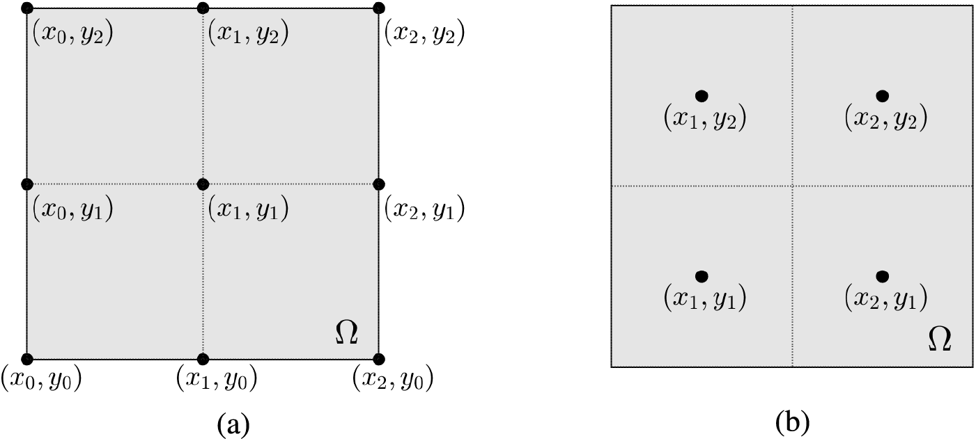
Figure 1: Schematic illustrations of (a) cell corner points and (b) cell center points on the computational domain
We can easily reduce or extend to one-dimensional and three-dimensional spaces.
When reviewing the numerical methods, we mainly focus on the accuracy and stability of the reviewed methods. High accuracy allows the user to predict phase separation dynamics in diblock copolymer systems with relatively low computational cost, such as coarse spatial grid or large time step. Therefore, high accuracy can lead to an effective numerical method. Stability is also concerned with time step and accuracy of the numerical method. High stability, and sometimes unconditional stability allows a larger time step to be used for the numerical simulation without the risk of blowing up. Therefore, we can obtain more freedom when modifying the time step size for a desired accuracy.
The FDM is a widely employed numerical technique for solving partial differential equations, known for its simplicity and broad applicability. A key advantage of this method is its ease of implementation for a range of problems with regular grid structures, making it particularly effective for time-dependent simulations. Although the accuracy of the method is influenced by grid resolution and step size, it can be refined to achieve higher precision. Despite some limitations in handling complex boundaries or irregular domains, the FDM remains a valuable tool due to its computational efficiency and straightforward implementation. Xiao et al. [47] developed a space-time fourth-order method for two- and three-dimensional CH type equations. The authors used the operator splitting method with auxiliary variables for spatial differentiation terms to enable multi-thread computation. In addition, we extended the numerical scheme for the phase-field diblock copolymer model. Numerical methods for solving systems of equations with nonlinear terms, such as the NCH equation, are primal and difficult problems [48]. Jeong et al. [22] conduct a numerical investigation on controlling local defectivity in self-assembled diblock copolymer patterns by designing suitable substrates. The numerical solution algorithm is described as follows. Considering trench domain
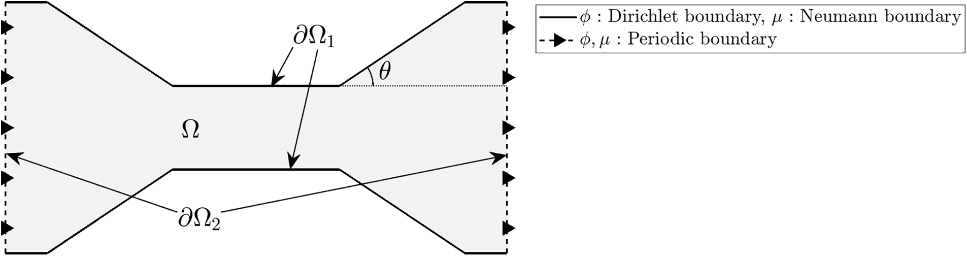
Figure 2: Schematic diagram of the computational domain
We discretize
where
We need to apply certain special formulas considering the boundary conditions. To facilitate understanding, we consider one example illustrated in Fig. 3. For the points
where
where
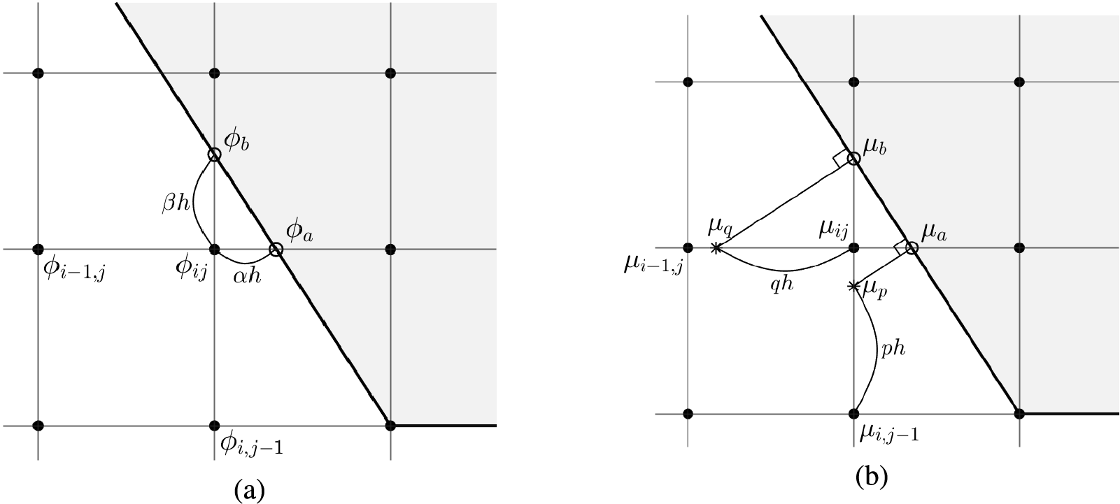
Figure 3: Schematic representation of (a) Dirichlet boundary condition and (b) Neumann boundary condition
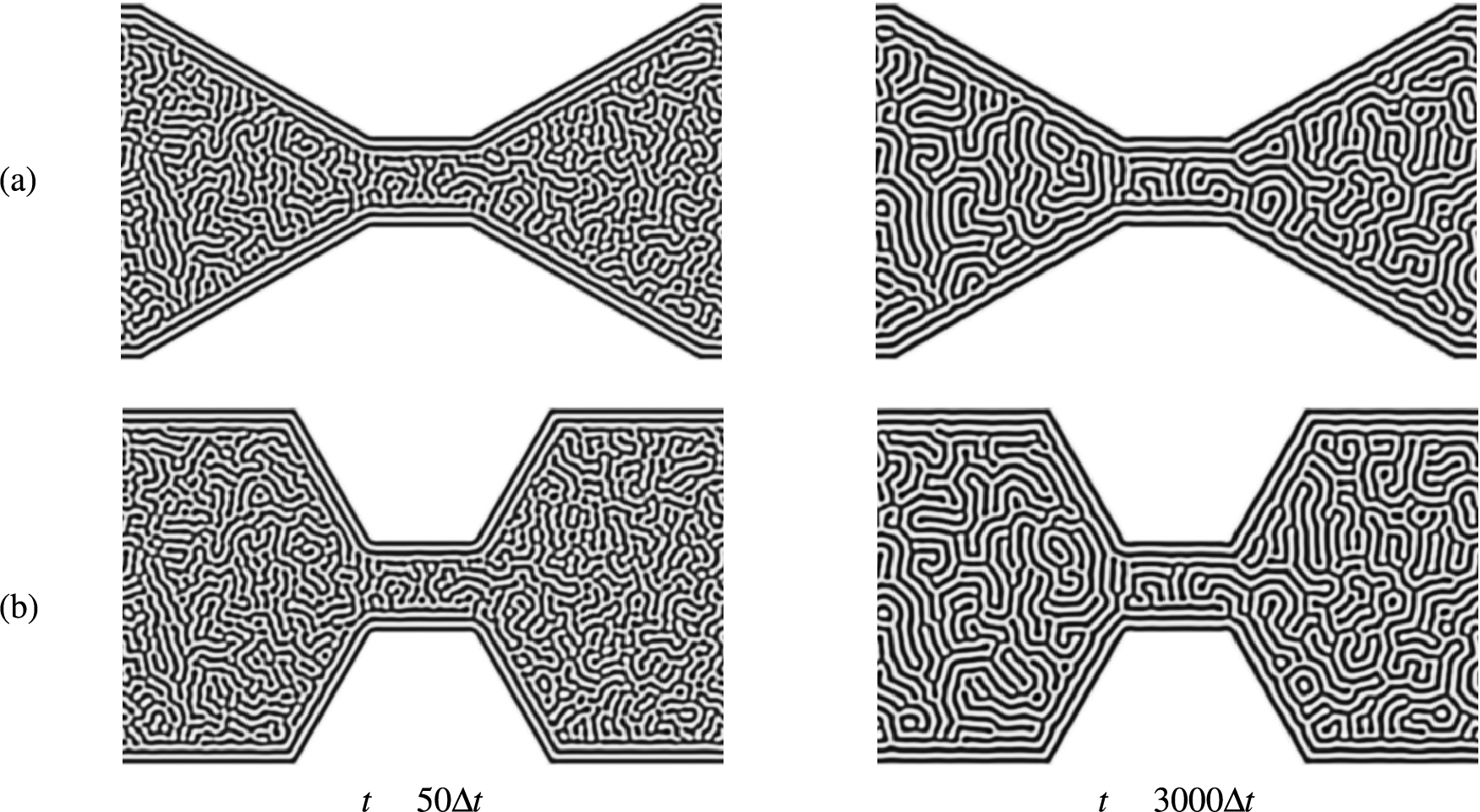
Figure 4: Snapshots of the numerical solutions with (a)
Jeong et al. [24] developed a numerical method to investigate microphase separation patterns in diblock copolymer melts on curved surfaces. This method employs a discrete narrow band grid adjacent to the curved surface and applies a pseudo-Neumann boundary condition for the near boundary using the closest point scheme. Therefore, the Laplace–Beltrami operator can be replaced with the standard Laplace operator. We define the
We define the discrete Laplace operator as
Then, we discretization the NCH Eqs. (1) and (2) by applying the unconditionally stable scheme.
The numerical closest point of
We use pseudo-Neumann boundary condition on
Fig. 5a,b shows schematic illustrations of the narrow band domain for the cross section of the sphere in three- and two-dimensions, respectively. Since
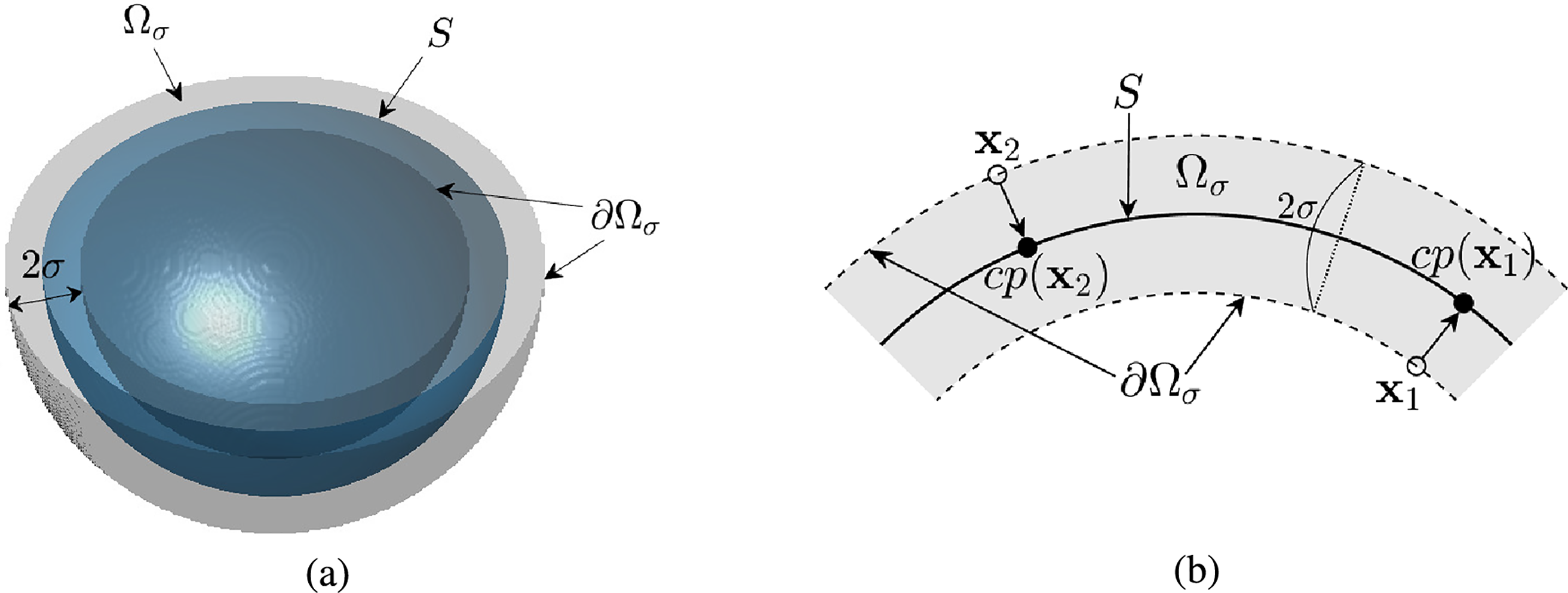
Figure 5: Schematic illustrations of (a) the narrow band domain for surface S and (b) the closest points for the boundary
Here, we iteratively compute Eqs. (15) and (16) until
Fig. 6 displays the temporal evolution of the computational solution for the bunny surface with initial conditions
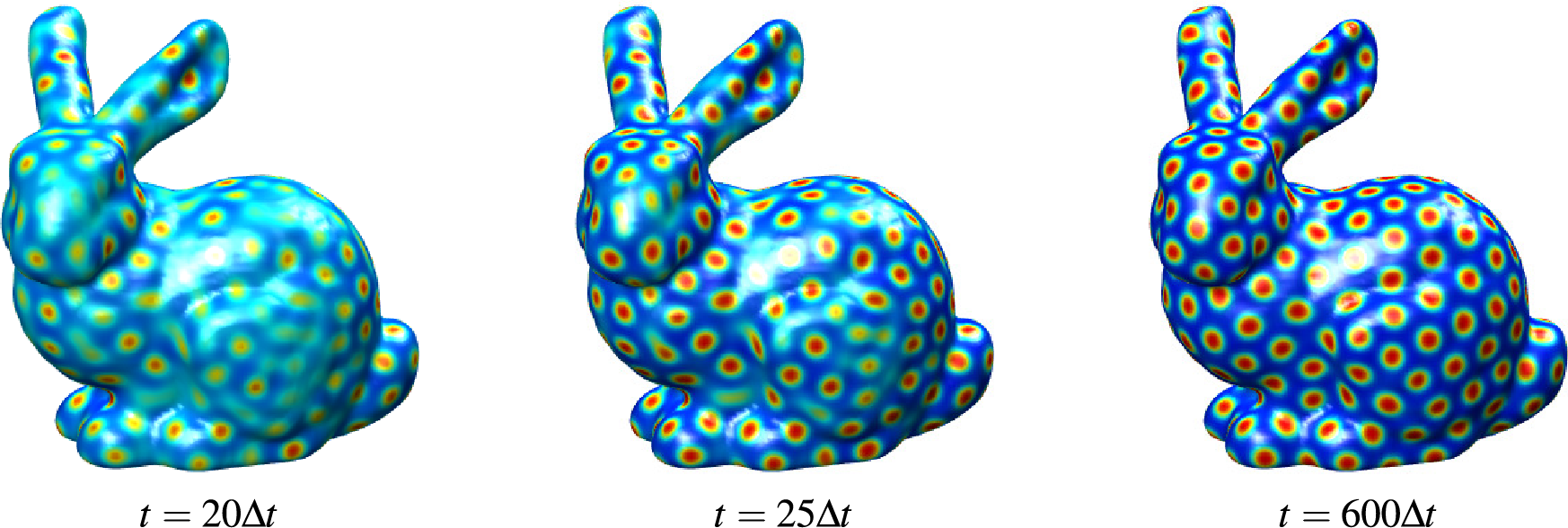
Figure 6: Snapshot of the numerical solution using the numerical algorithm from [24] at time
We observe that numerical simulation results form appropriate patterns in complex bunny surfaces. Yang [23] presented a linear time-marching scheme for the Ohta–Kawasaki model coupled with incompressible fluid flow, describing the phase-field model for diblock copolymers in fluid environments. The numerical algorithm employs the scalar auxiliary variable (SAV) approach, which ensures energy stability, even with large time steps. The 2D and 3D spatial discretizations are conducted using the FDM, providing a practical and efficient framework for computation. Furthermore, the authors analytically demonstrated the existence of unique solutions and proved the method’s energy stability.
The Fourier spectral method is a technique for solving partial differential equations, that approximates a solution using a sum of functions from a certain function space. To solve problems with periodic boundary conditions, use Fourier transformation composed of sine and cosine functions, and to solve problems with Neumann boundary conditions, use cosine transformation composed only of cosine functions. We consider only two dimensions, and for one or three dimensions it is easily derived from this. The Fourier transformation satisfies the periodic boundary condition, thus we define the discrete domain using the cell corner points. The discrete Fourier transform and its inverse transform are defined by
where
Thus, Laplacian is defined using Eqs. (19) and (20) as
Then, the linearly stabilized splitting method is used to the NCH equation as
where
Hence, we obtain the numerical solution in the Fourier space from Eq. (22) as
Then, we use the inverse discrete Fourier transform to obtain the computational solution
The Fourier spectral method based on discrete cosine transformation can be used to solve phase-field models with Neumann boundary conditions [51]. We define the computational discrete domain using the cell center points to describe the Fourier spectral method with discrete cosine transform. The discrete cosine transform and its inverse transform are defined by
where
where
Hence, similar to the Fourier spectral method with discrete Fourier transform, we can solve Eq. (21) using discrete cosine transformation. Xia et al. [52] employed a phase-field model within a Lagrange multiplier framework to investigate crystal phase transitions and nucleation processes, demonstrating the effectiveness of the Fourier spectral method in capturing complex phase dynamics. Li et al. [53] used the Fourier spectral method to solve biological transport networks in complex domains, providing insights into the optimization properties and adaptive mechanisms of network structures. Refer to [54] for detailed information. Fig. 7 shows the schematic illustrations of the discrete Fourier transform, the discrete cosine transform, and the discrete sine transform, from top to bottom. The dots on the x-axis represent the points of the discrete domain, while the dashed lines connecting the dots indicate the corresponding values of
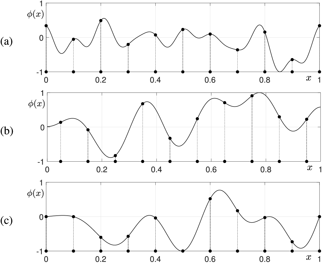
Figure 7: Schematic illustrations of (a) the discrete Fourier, (b) the discrete cosine, and (c) the discrete sine transforms
Jeong et al. [55] investigated the energy-minimizing wavelength in the equilibrium state of diblock copolymers in the hex-cylinder phase by solving the NCH equation using the Fourier spectral method with the discrete Fourier transform. The boundary condition is a periodic boundary condition with the discrete domain using the cell center point. The authors performed computations in rectangular domains with an aspect ratio of
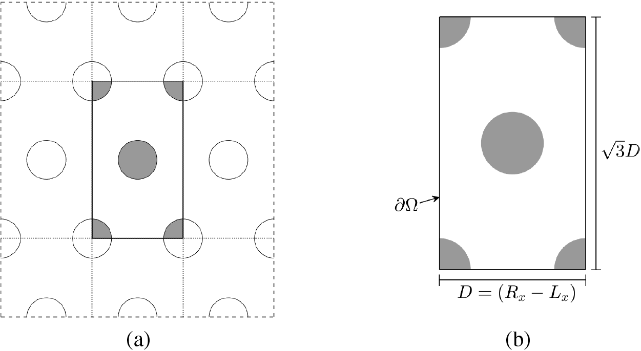
Figure 8: Schematic diagram of (a) the hexagonal pattern and (b) the domain with aspect ratio
At time
We perform the numerical test for the discrete total energy. For numerical simulation,
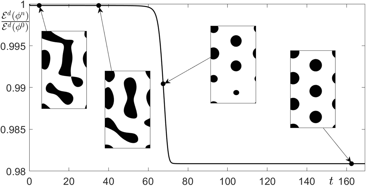
Figure 9: The discrete total energy with a snapshot of the numerical solutions
We observe the formation of a hexagonal pattern in the discrete equilibrium state and discrete total energy dissipation from numerical results. Chen et al. [56] presented a hydrodynamically-coupled phase-field model for diblock copolymer melts based on a conservative Allen–Cahn equation that preserves the volume fraction of the two monomers. In addition, the authors developed the linear and second-order time-marching method for the presented phase-field model. This method is easy to implement and can also be applied to a variety of phase-field models, such as CH equation for the diblock copolymer melts.
2.3 Alternating Direction Explicit
Yang et al. [57] developed an explicit FDM for the Ohta–Kawasaki model to describe microphase separation patterns in diblock copolymer melts. Their approach employs a Saul’yev-type scheme, which is grounded in a linearly stabilized convex splitting method, to achieve effective discretizations of the model equations. This method enhances the numerical stability of the simulations, allowing for more stable predictions of the complex behavior exhibited by diblock copolymer melts. The discrete domain is defined by using cell center points. The NCH Eqs. (1) and (2) are rewritten by applying the linear convex splitting-type scheme [58] as
where
Then, we use the Saul’yev-type method [59]. There are a total of 8 cases considering the order of
We can simplify Eq. (25) as
where
We consider the irregular domain
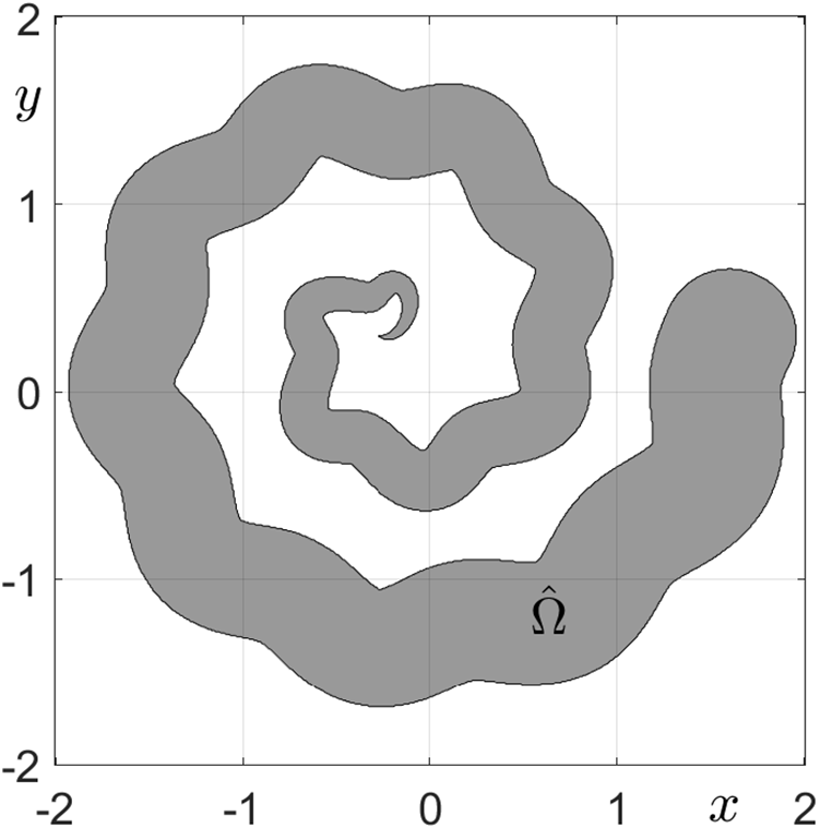
Figure 10: Schematic illustrations of the irregular domain
For the numerical test, we used parameters
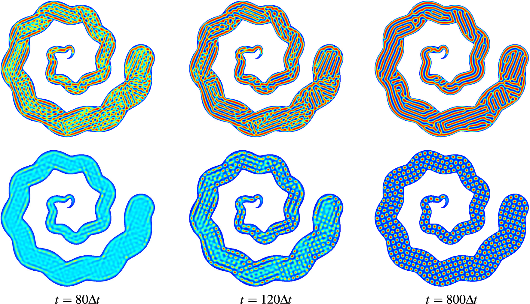
Figure 11: Pattern formations in irregular domain
Next, we perform numerical simulations to investigate how different boundary conditions, such as Dirichlet and Neumann boundary conditions, influence the simulation results. The initial condition is given by
Fig. 12 shows the numerical solutions obtained under different boundary conditions. From top to bottom, the results correspond to
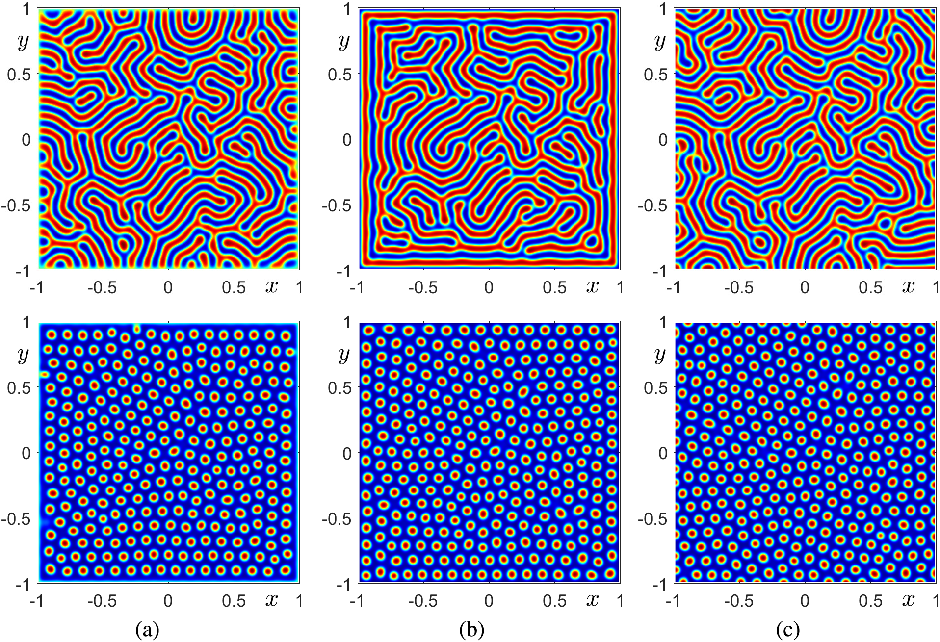
Figure 12: Numerical solutions at time
2.4 Invariant Energy Quadratization Approach
The invariant energy quadratization (IEQ) method is a numerical method designed to ensure energy stability when solving gradient flow problems. Originally proposed by Yang [60], the IEQ method transforms nonlinear partial differential equations into a form that allows for constructing energy-stable time-marching schemes. We simply describe an IEQ approach for the NCH equation. The auxiliary variable is defined as
We get
Therefore, we can obtain the energy dissipation law of the system (27)–(29) by taking the
The first-order time discretization IEQ method for the system (27)–(29) is defined by
The solution algorithms for the CH equation using the IEQ scheme is studied by Chen et al. [61], which are unconditionally stable. Two numerical methods, each first-order and second-order are reported. Numerical simulations showed that a large time step can be adopted while maintaining the energy decrease, therefore verifying the applicability of the proposed method.
2.5 Scalar Auxiliary Variable Approach
The SAV scheme was originally proposed by Shen et al. [62] and based on the IEQ approach, constructs energy-stable and efficient time discretization methods for gradient flows. The SAV scheme is applicable to different gradient flows and can be extended to higher-order by applying the backward differentiation formula (BDF) and Adam–Bashforth methods. We describe an SAV scheme for the NCH equation. The scalar auxiliary variable
where C is a non-negative constant, which guarantees the value beneath the square root is not zero. Thus, we have
Hence, we get
We take the
Zhang et al. [63] developed the stabilized SAV scheme for solving the CH phase field equation for diblock copolymers. The authors applied BDF2 to the SAV method for the NCH equation. We discretize the system (30)–(32) with respect to time.
where S is a positive stabilizing parameter,
where
Theorem 1. Suppose that
where
Proof. We take the
Then, we take the
From
Since
By multiplying (35) with
We consider two identities follows
Next, we combine the Eqs. (36)–(39) and by using the above two identities to get
We can rewrite the above equation using the definition of total free energy as
In the right-hand terms of the above equation, the sum of all terms except
Thus, the discrete system (33)–(35) satisfies the discrete energy emission law. □
Zhang et al. [64] expanded a magnetic-coupled diblock copolymer system by introducing a magnetic field in the CH equation for diblock copolymers. The authors developed the second-order time marching method using the stabilized SAV scheme to solve model. Wu et al. [65] developed a method with temporally second-order accuracy and unconditional energy stability based on the SAV approach scheme for a coupled CH system to simulate phase separation in the homopolymer and copolymer mixtures. In addition, the authors used the Fourier spectral method for space to minimize errors in space. Huang et al. [66] establish the error estimates of the SAV scheme for the coupled CH equation in the diblock copolymer. The numerical method is based on the SAV approach for time and the Fourier spectral method for space. Li et al. [67] applied the IEQ method to simulate anisotropic dendritic crystal growth with an azimuthal field, developing a second-order unconditionally energy-stable numerical scheme validated through simulations of complex growth processes. Jiang et al. [68] employed the SAV method to study fluid-surfactant systems on curved surfaces, demonstrating the precision and efficiency of their second-order, unconditionally energy-stable scheme. Lai et al. [69] extended the SAV method to analyze connected regions in digital models, proposing a stable and efficient algorithm for complex structure analysis. In [70], the authors proposed a conservative Allen–Cahn equation for diblock copolymers. They developed a numerical method based on the stabilized SAV scheme to solve the developed model. Through numerical tests, they validated the effectiveness of the new model by comparing it with the CH diblock copolymer model.
3 Applications of the Phase-Field Diblock Copolymer Model
The phase-field model for microphase separation patterns in diblock copolymer melts is widely applicable to various applications. Its capability to describe complex behaviors and microstructural patterns during phase separation makes it a valuable tool in materials science and polymer research. We present a detailed discussion on several examples, including fingerprint image restoration and 3D printing. Beyond these examples, the NCH equation has been widely applied in various fields, particularly in biology and materials science. In biology, the Green’s functionG from Eq. (4) plays a critical role in modeling cancer cell invasion [71] and solid tumor growth [72]. In materials science, the NCH equation has been particularly successful in describing diverse phenomena. Notable examples include mesoscopic models of particle dynamics for pattern formation [73] and phase transitions [74]. These examples highlight the versatility of the NCH equation across multiple disciplines.
3.1 Fingerprint Image Restoration
Lee et al. [75] presented a semi-automatic fingerprint image restoration algorithm using the NCH equation for the damaged fingerprint images. The developed fingerprint image restoration algorithm is based on the alternating direction explicit scheme [57]. Let
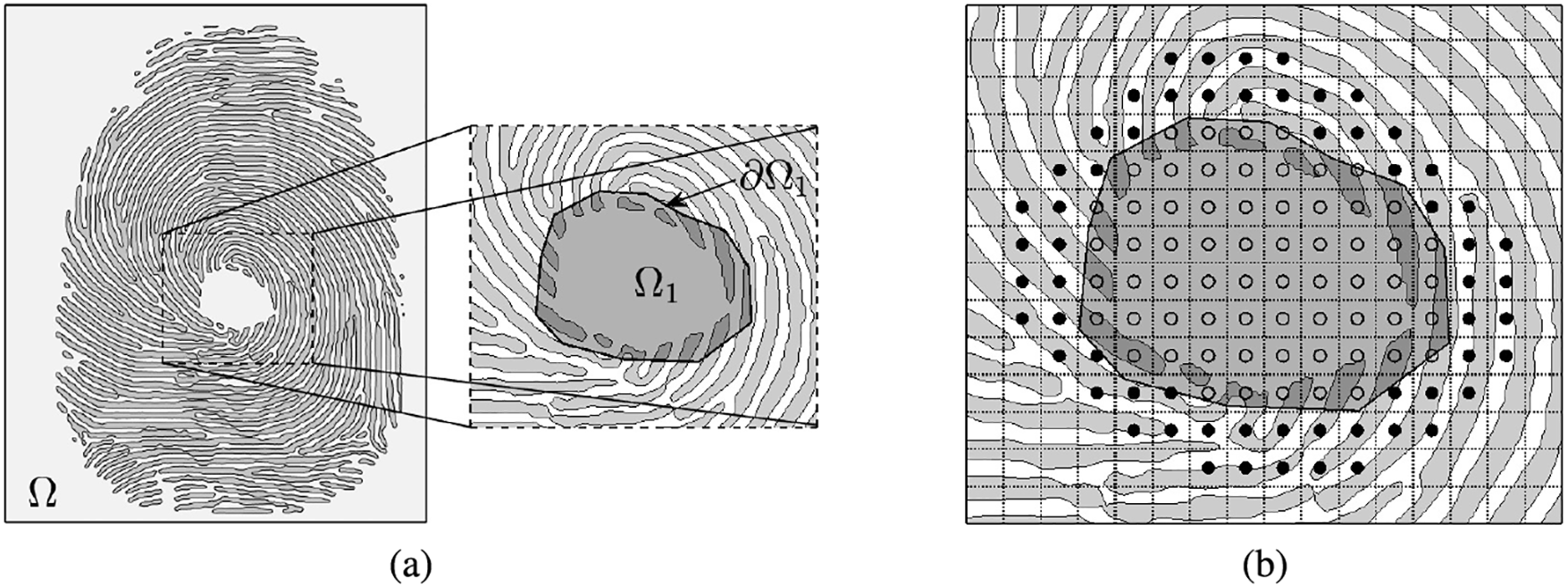
Figure 13: Schematic illustrations of (a) the global domain
We used the semi-automatic fingerprint image restoration algorithm based on the NCH equation to restore the damaged fingerprints. The main idea of the algorithm proposed by the authors is to find a spatial step size
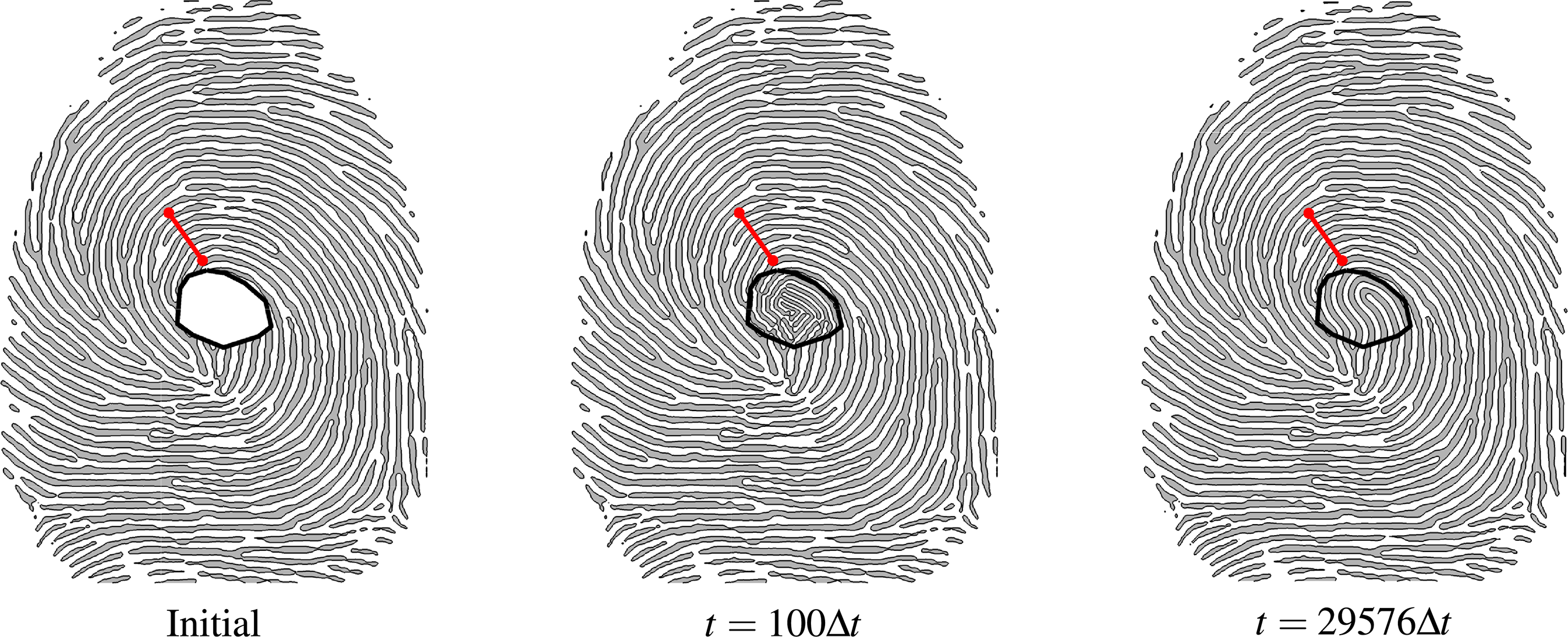
Figure 14: Numerical solution of the NCH equation using the semi-automatic fingerprint image restoration algorithm at times
Lee et al. [76] proposed a numerical method to generate a porous structure of arbitrary shape for 3D printing. The numerical method is based on the Fourier spectral method [55]. We used parameter
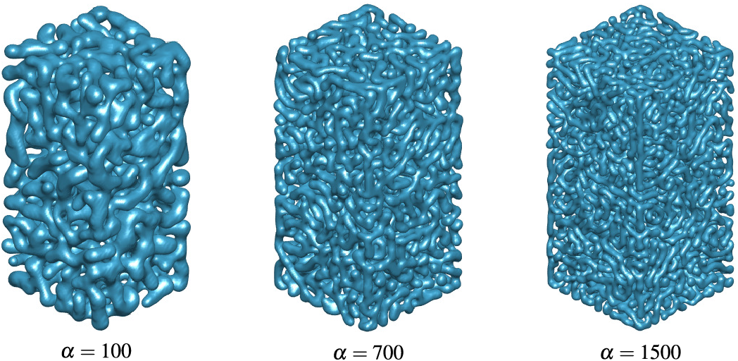
Figure 15: The
Various distance functions can be utilized to generate porous structures within other solid geometries that are not cubes. Please refer to [76]. The generation of porous structures has the advantage of controlling the shape of the porosity through the space-dependent average concentration function
Yoon et al. [77] presented a numerical algorithm to make uniformly distributed circular porous patterns on curved surfaces for 3D printing structures in 3D space using the computational method for the NCH equation [24]. The authors defined a narrow band domain including the surface to efficiently and simply solve the NCH equation, enabling the generation of circular porous patterns on the surface. Xia et al. [78] applied an unconditionally energy-stable numerical scheme to analyze the Swift–Hohenberg equation on arbitrary surfaces, achieving stable, second-order accurate results. Li et al. [79] developed a direct discretization technique to solve multicomponent CH systems on surfaces, yielding precise and stable solutions. Additionally, Xia et al. [80] introduced an unconditionally energy-stable phase-field approach for simulating binary thermal fluids on arbitrary surfaces with high accuracy. For numerical simulation, we used parameters
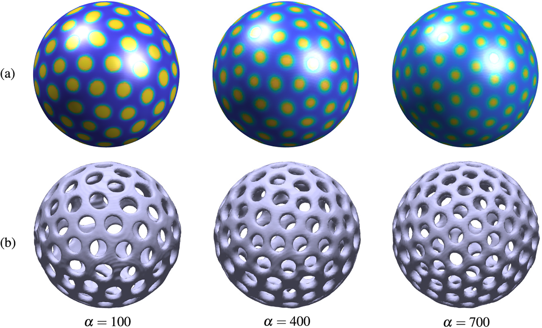
Figure 16: (a) Numerical solutions on the surface and (b) isosurfaces at
In this review paper, we extensively presented various numerical methods that model the phase separation dynamics of diblock copolymer melts through the phase-field model. Many applications adopted the diblock copolymer system to create and simulate the movement of phase boundaries of nanoscale complex structures. We examined five state-of-the-art numerical methods that solve the nonlocal Cahn–Hilliard equation. The finite difference method was simple to implement and broadly applicable. However, it had limitations in complex domains. On the other hand, the Fourier spectral method is suitable for solving models in complex domains, but is limited to specific boundary conditions and cell-centred grids. The alternating direction explicit method allowed more stable predictions on complex domains, but had to handle the error from splitting the governing equation. The invariant energy quadratization method proposed by Yang and the scalar auxiliary variable approach by Shen et al. showed their strength in energy stability. Furthermore, we introduce recent applications of the phase-field model such as Fingerprint image restoration and 3D printing to illustrate its versatility in different fields. Overall, this analysis serves as a valuable resource for researchers seeking to understand and apply numerical methods in the study of diblock copolymer melts.
Acknowledgement: The corresponding author (Junseok Kim) and coauthors express their gratitude to the reviewers for their valuable comments, which have enhanced the quality of this manuscript.
Funding Statement: The authors received no specific funding for this study.
Author Contributions: The authors confirm contribution to the paper as follows: study conception and design: Youngjin Hwang, Junseok Kim; methodology: Youngjin Hwang, Junseok Kim; software: Youngjin Hwang, Seungyoon Kang; visualization: Youngjin Hwang; formal analysis: Youngjin Hwang; validation: Youngjin Hwang, Seungyoon Kang; investigation: Youngjin Hwang, Seungyoon Kang; draft manuscript preparation: Youngjin Hwang, Seungyoon Kang, Junseok Kim; project administration: Junseok Kim; supervision: Junseok Kim; funding acquisition: Junseok Kim. All authors reviewed the results and approved the final version of the manuscript.
Availability of Data and Materials: The data that support the findings of this study are available from the corresponding author, Junseok Kim, upon reasonable request.
Ethics Approval: Not applicable.
Conflicts of Interest: The authors declare no conflicts of interest to report regarding the present study.
References
1. Ohta T, Kawasaki K. Equilibrium morphology of block copolymer melts. Macromolecules. 1986;19(10):2621–32. doi:10.1021/ma00164a028. [Google Scholar] [CrossRef]
2. Farrell PE, Pearson JW. A preconditioner for the Ohta-Kawasaki equation. SIAM J Matrix Analy Appl. 2017;38(1):217–25. doi:10.1137/16M1065483. [Google Scholar] [CrossRef]
3. Matsen MW, Schick M. Stable and unstable phases of a diblock copolymer melt. Phys Rev Lett. 1994;72(16):2660. doi:10.1103/PhysRevLett.72.2660. [Google Scholar] [PubMed] [CrossRef]
4. Fish J, Wagner GJ, Keten S. Mesoscopic and multiscale modelling in materials. Nature Mat. 2021;20(6):774–86. doi:10.1038/s41563-020-00913-0. [Google Scholar] [PubMed] [CrossRef]
5. Chen LQ. Phase-field models for microstructure evolution. Ann Rev Mat Res. 2002;32(1):113–40. doi:10.1146/annurev.matsci.32.112001.132041. [Google Scholar] [CrossRef]
6. Van Den Berg JB, Williams J. Rigorously computing symmetric stationary states of the Ohta-Kawasaki problem in three dimensions. SIAM J Mathem Anal. 2019;51(1):131–58. doi:10.1137/17M1155624. [Google Scholar] [CrossRef]
7. Barros GF, Côrtes AM, Coutinho AL. Finite element solution of nonlocal Cahn-Hilliard equations with feedback control time step size adaptivity. Int J Num Meth Eng. 2021;122(18):5028–52. doi:10.1002/nme.6755. [Google Scholar] [CrossRef]
8. Cao L, Ghattas O, Oden JT. A globally convergent modified newton method for the direct minimization of the ohta-kawasaki energy with application to the directed self-assembly of diblock copolymers. SIAM J Sci Comput. 2022;44(1):B51–79. doi:10.1137/20M1378119. [Google Scholar] [CrossRef]
9. Singh PK, Cao L, Tan J, Faghihi D. A nonlocal theory of heat transfer and micro-phase separation of nanostructured copolymers. Int J Heat Mass Transf. 2023;215(1):124474. doi:10.1016/j.ijheatmasstransfer.2023.124474. [Google Scholar] [CrossRef]
10. Yasen W, Dong R, Aini A, Zhu X. Recent advances in supramolecular block copolymers for biomedical applications. J Mat Chem B. 2020;8(36):8219–31. doi:10.1039/D0TB01492C. [Google Scholar] [PubMed] [CrossRef]
11. Iqbal MJ, Soomro I, Razzaq MA, Martinez EO, Martinez ZLV, Ashraf I. Investigation of structural frustration in symmetric diblock copolymers confined in polar discs through cell dynamic simulation. Sci Rep. 2024;14(1):25916. doi:10.1038/s41598-024-76213-3. [Google Scholar] [PubMed] [CrossRef]
12. Feng J, Ruckenstein E. Self-assembling of hydrophobic-hydrophilic copolymers in hydrophobic nanocylindrical tubes: formation of channels. J Chem Phys. 2008;128(7):074903. doi:10.1063/1.2831510. [Google Scholar] [PubMed] [CrossRef]
13. Weyersberg A, Vilgis TA. Phase transitions in diblock copolymers: theory and Monte Carlo simulations. Phys Rev E. 1993;48(1):377. doi:10.1103/PhysRevE.48.377. [Google Scholar] [PubMed] [CrossRef]
14. Dreyer O, Ibbeken G, Schneider L, Blagojevic N, Radjabian M, Abetz V, et al. Simulation of solvent evaporation from a diblock copolymer film: orientation of the cylindrical mesophase. Macromolecules. 2022;55(17):7564–82. doi:10.1021/acs.macromol.2c00612. [Google Scholar] [CrossRef]
15. Gee RH, Lacevic N, Fried LE. Atomistic simulations of spinodal phase separation preceding polymer crystallization. Nature Mat. 2006;5(1):39–43. doi:10.1038/nmat1543. [Google Scholar] [PubMed] [CrossRef]
16. Leibler L. Theory of microphase separation in block copolymers. Macromolecules. 1980;13(6):1602–17. doi:10.1021/ma60078a047. [Google Scholar] [CrossRef]
17. Xu W, Jiang K, Zhang P, Shi AC. A strategy to explore stable and metastable ordered phases of block copolymers. J Phy Chem B. 2013;117(17):5296–305. doi:10.1021/jp309862b. [Google Scholar] [PubMed] [CrossRef]
18. Pezzutti AD, Hernández H. Unconditionally stable algorithm for copolymer and copolymer-solvent systems. Pap Phy. 2020;12:120001. doi:10.4279/pip.120001. [Google Scholar] [CrossRef]
19. Kravchenko VS, Abetz V, Potemkin II. Self-assembly of gradient copolymers in a selective solvent. New structures and comparison with diblock and statistical copolymers. Polymer. 2021;235:124288. doi:10.1016/j.polymer.2021.124288. [Google Scholar] [CrossRef]
20. Chen T, Zhang Y, Xiao S, Yao D, Jiang W, Liang H. Catalytic assembly of symmetric diblock copolymers in a thin film: a dissipative particle dynamics simulation study. Phy Chem Chem Phy. 2023;25(14):9779–84. doi:10.1039/D3CP00447C. [Google Scholar] [PubMed] [CrossRef]
21. Tomiyoshi Y, Oya Y, Kawakatsu T, Okabe T. Reaction-induced morphological transitions in a blend of diblock copolymers and reactive monomers: dissipative particle dynamics simulation. Soft Matter. 2024;20(1):124–32. doi:10.1039/D3SM00959A. [Google Scholar] [PubMed] [CrossRef]
22. Jeong D, Choi Y, Kim J. Numerical investigation of local defectiveness control of diblock copolymer patterns. Conden Matter Phy. 2016;19(3):33001. doi:10.5488/CMP.19.33001. [Google Scholar] [CrossRef]
23. Yang J. Linear energy-stable method with correction technique for the Ohta-Kawasaki–Navier-Stokes model of incompressible diblock copolymer melt. Commun Nonlinear Sci Numer Simul. 2024;131(1):101906. doi:10.1016/j.cnsns.2024.107835. [Google Scholar] [CrossRef]
24. Jeong D, Kim J. Microphase separation patterns in diblock copolymers on curved surfaces using a nonlocal Cahn-Hilliard equation. Eur Phy J E. 2015;38(11):1–7. doi:10.1140/epje/i2015-15117-1. [Google Scholar] [PubMed] [CrossRef]
25. Muramatsu M, Yashiro K, Kawada T, Terada K. Simulation of ferroelastic phase formation using phase-field model. Int J Mech Sci. 2018;146:462–74. doi:10.1016/j.ijmecsci.2017.12.027. [Google Scholar] [CrossRef]
26. Momeni K, Ji Y, Wang Y, Paul S, Neshani S, Yilmaz DE, et al. Multiscale computational understanding and growth of 2D materials: a review. NPJ Comp Mater. 2020;6(1):22. doi:10.1038/s41524-020-0280-2. [Google Scholar] [CrossRef]
27. Endo K, Matsuda Y, Tanaka S, Muramatsu M. A phase-field model by an Ising machine and its application to the phase-separation structure of a diblock polymer. Sci Rep. 2022;12(1):10794. doi:10.1038/s41598-022-14735-4. [Google Scholar] [PubMed] [CrossRef]
28. Shen X, Wang Q. Thermodynamically consistent algorithms for models of diblock copolymer solutions interacting with electric and magnetic fields. J Sci Comput. 2021;88(2):43. doi:10.1007/s10915-021-01470-7. [Google Scholar] [CrossRef]
29. Adibi T, Ahmed SF, Razavi SE, Adibi O, Badruddin IA, Javed S. Impact of artificial compressibility on the numerical solution of incompressible nanofluid flow. Comput, Mat Cont. 2023;74(3):5123–39. doi:10.32604/cmc.2023.034008. [Google Scholar] [CrossRef]
30. Song X, Xia Q, Kim J, Li Y. An unconditional energy stable data assimilation scheme for Navier-Stokes–Cahn-Hilliard equations with local discretized observed data. Comput Math Appl. 2024;164(10):21–33. doi:10.1016/j.camwa.2024.03.018. [Google Scholar] [CrossRef]
31. Song X, Xia B, Li Y. An efficient data assimilation based unconditionally stable scheme for Cahn-Hilliard equation. Comput Appl Math. 2024;43(3):121. doi:10.1007/s40314-024-02632-7. [Google Scholar] [CrossRef]
32. Martínez Agustín F, Ruiz Salgado S, Zenteno Mateo B, Rubio E, Morales M. 3D pattern formation from coupled Cahn-Hilliard and Swift-Hohenberg equations: morphological phases transitions of polymers, bock and diblock copolymers. Comput Mater Sci. 2022;210(5):111431. doi:10.1016/j.commatsci.2022.111431. [Google Scholar] [CrossRef]
33. Barua AK, Chew R, Li S, Lowengrub J, Münch A, Wagner B. Sharp-interface problem of the Ohta-Kawasaki model for symmetric diblock copolymers. J Comput Phys. 2023;481(10):112032. doi:10.1016/j.jcp.2023.112032. [Google Scholar] [CrossRef]
34. Meng X, Cheng A, Liu Z. The high-order exponential semi-implicit scalar auxiliary variable approach for the general nonlocal Cahn-Hilliard equation. Commun Nonlinear Sci Numer Simul. 2024;137:108169. doi:10.1016/j.cnsns.2024.108169. [Google Scholar] [CrossRef]
35. Elbar C, Perthame B, Poiatti A, Skrzeczkowski J. Nonlocal Cahn-Hilliard equation with degenerate mobility: incompressible limit and convergence to stationary states. Arch Ration Mech Anal. 2024;248(3):41. doi:10.1007/s00205-024-01990-0. [Google Scholar] [CrossRef]
36. Wu XF, Dzenis YA. Phase-field modeling of the formation of lamellar nanostructures in diblock copolymer thin films under inplanar electric fields. Phy Rev E-Statist, Nonlin Soft Matt Phy. 2008;77(3):031807. doi:10.1103/PhysRevE.77.031807. [Google Scholar] [PubMed] [CrossRef]
37. Cheng Q, Yang X, Shen J. Efficient and accurate numerical schemes for a hydro-dynamically coupled phase field diblock copolymer model. J Computat Phy. 2017;341(9):44–60. doi:10.1016/j.jcp.2017.04.010. [Google Scholar] [CrossRef]
38. Chen L, Ma Y, Ren B, Zhang G. Numerical approximations of diblock copolymer model using a modified leapfrog time-marching scheme. Computation. 2023;11(11):215. doi:10.3390/computation11110215. [Google Scholar] [CrossRef]
39. Li T, Liu P, Zhang J, Yang X. Efficient Fully decoupled and second-order time-accurate scheme for the Navier-Stokes coupled Cahn-Hilliard Ohta-Kawaski Phase-Field model of Diblock copolymer melt. J Comput Appl Math. 2022;403(10):113843. doi:10.1016/j.cam.2021.113843. [Google Scholar] [CrossRef]
40. Wang Y, Xiao X, Zhang H, Qian X, Song S. Efficient diffusion domain modeling and fast numerical methods for diblock copolymer melt in complex domains. Comput Phys Commun. 2024;305(8):109343. doi:10.1016/j.cpc.2024.109343. [Google Scholar] [CrossRef]
41. Bensimon D, Kadanoff LP, Liang S, Shraiman BI, Tang C. Viscous flows in two dimensions. Rev Mod Phys. 1986;58(4):977. doi:10.1103/RevModPhys.58.977. [Google Scholar] [CrossRef]
42. Cao J, Zhang J, Yang X. Fully-decoupled and second-order time-accurate scheme for the cahn-hilliard ohta-kawaski phase-field model of diblock copolymer melt confined in hele-shaw cell. Commun Mathem Statist. 2024;12(3):479–504. doi:10.1007/s40304-022-00298-3. [Google Scholar] [CrossRef]
43. Xu Z, Han Y, Yin J, Yu B, Nishiura Y, Zhang L. Solution landscapes of the diblock copolymer-homopolymer model under two-dimensional confinement. Phys Rev E. 2021;104(1):014505. doi:10.1103/PhysRevE.104.014505. [Google Scholar] [PubMed] [CrossRef]
44. Zhang H, Liu L, Qian X, Song S. Large time-stepping, delay-free, and invariant-set-preserving integrators for the viscous Cahn-Hilliard–Oono equation. J Comput Phys. 2024;499(2):112708. doi:10.1016/j.jcp.2023.112708. [Google Scholar] [CrossRef]
45. Luo W, Zhao Y. Asymptotically compatible schemes for nonlocal Ohta-Kawasaki model. Numer Methods Partial Differ Equ. 2024;40(6):e23143. doi:10.1002/num.23143. [Google Scholar] [CrossRef]
46. Iqbal MJ, Soomro I, Mahar MH, Gulzar U. Exploring long-range order in diblock copolymers through cell dynamic simulations. VFAST Transact Softw Eng. 2024;12(2):31–45. doi:10.21015/vtse.v12i2.1795. [Google Scholar] [CrossRef]
47. Xiao X, Feng X, Shi Z. Efficient numerical simulation of Cahn-Hilliard type models by a dimension splitting method. Comput Mathem Appl. 2023;136(6):54–70. doi:10.1016/j.camwa.2023.01.037. [Google Scholar] [CrossRef]
48. Shams M, Kausar N, Ahmed SF, Badruddin IA, Javed S. Efficient numerical scheme for solving large system of nonlinear equations. Comput Mater Contin. 2023;74(3):5331–47. doi:10.32604/cmc.2023.033528. [Google Scholar] [CrossRef]
49. Eyre DJ. Unconditionally gradient stable time marching the Cahn-Hilliard equation. MRS Online Proc Libr (OPL). 1998;529:39. doi:10.1557/PROC-529-39. [Google Scholar] [CrossRef]
50. Semendyayev IBK, Mühlig GMH. Handbook of mathematics. 3rd ed. Berlin/Heidelberg, Germany: Springer; 1997. [Google Scholar]
51. Kim J, Kwak S, Lee HG, Hwang Y, Ham S. A maximum principle of the Fourier spectral method for diffusion equations. Electr Res Arch. 2023;31(9):5396–405. doi:10.3934/era.2023273. [Google Scholar] [CrossRef]
52. Xia Q, Yang J, Kim J, Li Y. On the phase field based model for the crystalline transition and nucleation within the Lagrange multiplier framework. J Comput Phys. 2024;513(336):113158. doi:10.1016/j.jcp.2024.113158. [Google Scholar] [CrossRef]
53. Li Y, Lv Z, Xia Q. On the adaption of biological transport networks affected by complex domains. Phys Fluids. 2024;36(10):101906. doi:10.1063/5.0231079. [Google Scholar] [CrossRef]
54. Hwang Y, Ham S, Lee HG, Kim H, Kim J. Numerical algorithms for the phase-field models using discrete cosine transform. Mech Res Commun. 2024;139:104305. doi:10.1016/j.mechrescom.2024.104305. [Google Scholar] [CrossRef]
55. Jeong D, Lee S, Choi Y, Kim J. Energy-minimizing wavelengths of equilibrium states for diblock copolymers in the hex-cylinder phase. Curr Appl Phy. 2015;15(7):799–804. doi:10.1016/j.cap.2015.04.033. [Google Scholar] [CrossRef]
56. Chen C, Zhang J, Yang X. Efficient numerical scheme for a new hydrodynamically-coupled conserved Allen-Cahn type Ohta-Kawaski phase-field model for diblock copolymer melt. Comput Phys Commun. 2020;256(10):107418. doi:10.1016/j.cpc.2020.107418. [Google Scholar] [CrossRef]
57. Yang J, Lee C, Jeong D, Kim J. A simple and explicit numerical method for the phase-field model for diblock copolymer melts. Comput Mater Sci. 2022;205(3):111192. doi:10.1016/j.commatsci.2022.111192. [Google Scholar] [CrossRef]
58. Shin J, Lee HG, Lee JY. Convex splitting Runge-Kutta methods for phase-field models. Comput Mathem Appl. 2017;73(11):2388–403. doi:10.1016/j.camwa.2017.04.004. [Google Scholar] [CrossRef]
59. Dehghan M. Saulyev’s techniques for solving a parabolic equation with a non linear boundary specification. Int J Comput Mathem. 2003;80(2):257–65. doi:10.1080/00207160304670. [Google Scholar] [CrossRef]
60. Yang X. Linear, first and second-order, unconditionally energy stable numerical schemes for the phase field model of homopolymer blends. J Computat Phy. 2016;327(4):294–316. doi:10.1016/j.jcp.2016.09.029. [Google Scholar] [CrossRef]
61. Chen R, Gu S. On novel linear schemes for the Cahn-Hilliard equation based on an improved invariant energy quadratization approach. J Comput Appl Math. 2022;414:114405. doi:10.1016/j.cam.2022.114405. [Google Scholar] [CrossRef]
62. Shen J, Xu J, Yang J. The scalar auxiliary variable (SAV) approach for gradient flows. J Computat Phy. 2018;353(11):407–16. doi:10.1016/j.jcp.2017.10.021. [Google Scholar] [CrossRef]
63. Zhang J, Chen C, Yang X. Efficient and energy stable method for the Cahn-Hilliard phase-field model for diblock copolymers. Appl Numer Mathem. 2020;151(1):263–81. doi:10.1016/j.apnum.2019.12.006. [Google Scholar] [CrossRef]
64. Zhang J, Yang X. A new magnetic-coupled Cahn-Hilliard phase-field model for diblock copolymers and its numerical approximations. Appl Math Lett. 2020;107(9):106412. doi:10.1016/j.aml.2020.106412. [Google Scholar] [CrossRef]
65. Wu J, Zhang X, Tan Z. An unconditionally energy stable algorithm for copolymer-homopolymer mixtures. Int J Mech Sci. 2023;238(6):107846. doi:10.1016/j.ijmecsci.2022.107846. [Google Scholar] [CrossRef]
66. Huang J, Ji G. Error estimates of the sav method for the coupled Cahn-Hilliard system in copolymer/homopolymer mixtures. Commun Mathem Sci. 2023;21(7):1895–916. doi:10.4310/CMS.2023.v21.n7.a7. [Google Scholar] [CrossRef]
67. Li Y, Qin K, Xia Q, Kim J. A second-order unconditionally stable method for the anisotropic dendritic crystal growth model with an orientation-field. Appl Numer Mathem. 2023;184(1):512–26. doi:10.1016/j.apnum.2022.11.006. [Google Scholar] [CrossRef]
68. Jiang B, Xia Q, Kim J, Li Y. Efficient second-order accurate scheme for fluid-surfactant systems on curved surfaces with unconditional energy stability. Commun Nonlinear Sci Numer Simul. 2024;135(32):108054. doi:10.1016/j.cnsns.2024.108054. [Google Scholar] [CrossRef]
69. Lai S, Jiang B, Xia Q, Xia B, Kim J, Li Y. On the phase-field algorithm for distinguishing connected regions in digital model. Eng Anal Bound Elem. 2024;168(2):105918. doi:10.1016/j.enganabound.2024.105918. [Google Scholar] [CrossRef]
70. Geng S, Li T, Ye Q, Yang X. A new conservative Allen-Cahn type Ohta-Kawaski phase-field model for diblock copolymers and its numerical approximations. Adv Appl Math Mech. 2022;14(1):101–24. doi:10.4208/aamm.OA-2020-0293. [Google Scholar] [CrossRef]
71. Gerisch A, Chaplain MA. Mathematical modelling of cancer cell invasion of tissue: local and non-local models and the effect of adhesion. J Theore Bio. 2008;250(4):684–704. doi:10.1016/j.jtbi.2007.10.026. [Google Scholar] [PubMed] [CrossRef]
72. Chauviere A, Hatzikirou H, Kevrekidis IG, Lowengrub JS, Cristini V. Dynamic density functional theory of solid tumor growth: preliminary models. AIP Adv. 2012;2(1):11210. doi:10.1063/1.3699065. [Google Scholar] [PubMed] [CrossRef]
73. Horntrop DJ, Katsoulakis MA, Vlachos DG. Spectral methods for mesoscopic models of pattern formation. J Computat Phy. 2001;173(1):364–90. doi:10.1006/jcph.2001.6883. [Google Scholar] [CrossRef]
74. Fife P. Some nonclassical trends in parabolic and parabolic-like evolutions. In: Kirkilionis M, Krömker S, Rannacher R, Tomi F, editors. Trends in nonlinear analysis. Berlin, Heidelberg: Springer; 2003. doi:10.1007/978-3-662-05281-5. [Google Scholar] [CrossRef]
75. Lee C, Kim S, Kwak S, Hwang Y, Ham S, Kang S, et al. Semi-automatic fingerprint image restoration algorithm using a partial differential equation. AIMS Mathematics. 2023;8(11):27528–41. doi:10.3934/math.20231408. [Google Scholar] [CrossRef]
76. Lee C, Jeong D, Yoon S, Kim J. Porous three-dimensional scaffold generation for 3D printing. Mathematics. 2020;8(6):946. doi:10.3390/math8060946. [Google Scholar] [CrossRef]
77. Yoon S, Lee C, Park J, Jeong D, Kim J. Uniformly distributed circular porous pattern generation on surface for 3d printing. Numer Mathem-Theory Meth Appl. 2020;13(4):845–62. [Google Scholar]
78. Xia B, Xi X, Yu R, Zhang P. Unconditional energy-stable method for the Swift-Hohenberg equation over arbitrarily curved surfaces with second-order accuracy. Appl Numer Mathem. 2024;198:192–201. doi:10.1016/j.apnum.2024.01.005. [Google Scholar] [CrossRef]
79. Li Y, Liu R, Xia Q, He C, Li Z. First-and second-order unconditionally stable direct discretization methods for multi-component Cahn-Hilliard system on surfaces. J Comput Appl Math. 2022;401:113778. doi:10.1016/j.cam.2021.113778. [Google Scholar] [CrossRef]
80. Xia Q, Liu Y, Kim J, Li Y. Binary thermal fluids computation over arbitrary surfaces with second-order accuracy and unconditional energy stability based on phase-field model. J Comput Appl Math. 2023;433:115319. doi:10.1016/j.cam.2023.115319. [Google Scholar] [CrossRef]
Cite This Article
 Copyright © 2025 The Author(s). Published by Tech Science Press.
This work is licensed under a Creative Commons Attribution 4.0 International License , which permits unrestricted use, distribution, and reproduction in any medium, provided the original work is properly cited.
 Downloads
 Citation Tools