Improved Cyclic System Based Optimization Algorithm (ICSBO)

1  Introduction

Optimization problems widely exist in production and life, such as optimizing the transportation path to reduce logistics and distribution costs and allocating funds to different investment projects in the financial field to maximize the return under the premise of controllable risk. Traditional optimization methods such as least squares and most rapid descent, generally for structured problems, have a clearer description of the problem and conditions, whereas the meta heuristic algorithms (MHAs) for a more universal description of the problem generally lack structural information. Moreover, MHAs have the characteristics of flexible structure, high stability, and satisfactory robustness, which make them the most effective methods for solving optimization problems.

As optimization problems become more complex, traditional MHAs, including genetic algorithms and differential algorithms, often exhibit limitations in convergence speed and accuracy. To address these challenges and enhance the solution quality for complex optimization tasks, many novel MHAs have been developed. In 2022, Ghasemi et al. proposed a new MHA, namely, circulatory-system-based optimization (CSBO), by modeling the human circulatory system [1]. Extensive experiments have demonstrated that CSBO outperforms biogeographic optimization algorithms [2], particle swarm optimization (PSO) algorithms, artificial bee colony algorithms [3], and other MHAs in both convergence speed and accuracy. Nevertheless, CSBO continues to face challenges, such as reduced convergence speed and susceptibility to local optima, when addressing high-dimensional, multi-peak complex optimization problems.

To address these challenges, this paper proposes an improved circulatory-system-based optimization (ICSBO) algorithm, with the following motivations and contributions:

(1) In the venous blood circulation mechanism of CSBO, individuals not only learn from themselves and other individuals but are also influenced by perturbations from other individuals. To ensure the evolutionary direction of the entire population, mutual learning should play a guiding role in the evolution of individuals, and the degree of learning through mutual interaction should be higher than that of perturbation-based learning. On this basis, a new venous blood circulation mechanism by adjusting the learning degree of perturbation-based learning is proposed.

(2) Given the advantage of the simplex method in fast convergence, it is incorporated into the updating mechanism of systemic circulation, which accelerates the convergence speed and accuracy of the population in the systemic circulation phase.

(3) Random perturbation in the pulmonary circulation can exhibit randomness, so it is prone to ineffective searches that fail to supplement diversity effectively. Because different search mechanisms can enhance the algorithm’s ability to handle various optimization problems, and the simplex method offers fast convergence while opposition-based learning can introduce more population diversity, both search mechanisms are incorporated into the pulmonary circulation strategy. This approach ensures the population’s convergence speed while providing greater diversity.

(4) MHAs are generally very susceptible to the situation where the overall diversity of a population is still good but distinct individuals remain unchanged for many consecutive generations during population evolution. Although the regeneration approach helps replenish diversity, it completely abandons the previous evolution of the individual. Individuals that outperform the previous generation in the evolution are stored in an archive. When an individual falls into local stagnation of updating, a historical individual is randomly selected from the archive to replace it, and a mechanism to replenish the diversity of population based on the external archive is proposed.

Experimental results on the CEC2017 test set demonstrate that the proposed ICSBO outperforms eight representative optimization algorithms, showcasing notable advantages in convergence speed, accuracy, and stability.

2  Related Work

MHA is a class of computational intelligence-based mechanism for solving complex optimization problems with optimal or satisfactory solutions, also known as intelligent optimization algorithms. MHA designs an intelligent iterative search by simulating relevant behaviors, functions, and mechanisms in biological, physical, chemical, and other systems or domains. MHA is widely used in many practical engineering fields because it has good global search capability and flexibility, and it does not require the optimization problem to have a functional form such as differentiable and derivable.

Metaheuristic algorithms are generally classified into four main groups according to their foundational principles: (1) Evolution-inspired algorithms, such as Genetic Algorithm (GA) [4], Differential Evolution (DE) [5], and Co-evolutionary Algorithms [6]; (2) Population-based methods, including Ant Colony Optimization (ACO) [7], Grey Wolf Optimizer (GWO) [8], Butterfly Optimization Algorithm (BOA) [9], and Great White Shark Algorithm [10]. (3) Algorithms based on physical phenomena, such as Simulated Annealing (SA) and Archimedes Optimization Algorithm [11]; (4) Algorithms based on human activities, such as Teaching-Learning-Based Optimization (TLBO) [12], Knowledge Sharing Algorithm (KSA) [13] and Information acquisition optimizer (IAO) [14].

However, MHAs still face challenges, such as slow convergence speed and a tendency to get trapped in local optima, when applied to high-dimensional, multi-peak complex optimization problems. To obtain the optimal solution of this kind of optimization problem, scholars have studied MHAs from two aspects.

On one hand, improving existing traditional heuristic algorithms to further enhance their optimization performance has been a focus of research. In 2023, Yao et al. developed an Enhanced Serpent Optimizer (ESO) [15] by integrating a new dynamic mechanism and an opposition-based learning strategy, aiming to enhance the Serpent Optimizer for solving practical engineering problems. In the same year, Wang et al. introduced an Improved Archimedes Optimization Algorithm (IAOA) [16], which employs the simplex method to adjust individuals with low fitness, enhancing the algorithm’s convergence speed and accuracy. Hu et al. (2023) introduced the Improved Orca Predation Algorithm (IOPA) [17], which enhances population diversity and helps the algorithm escape local minima by integrating a dimension-learning strategy with an opposition-based learning method. In 2024, Ye et al. proposed a multi-strategy enhanced dung beetle optimization algorithm (MDBO) [18], incorporating Latin hypercube sampling, lens imaging-based opposition learning, and dimension-wise optimization strategies to address issues such as poor diversity and unsatisfactory convergence speed. Furthermore, Nadimi-Shahraki et al. proposed the MTV-SCA (Multiple Trial Vectors Sine Cosine Algorithm) [19], which integrates multiple trial vectors along with four different search strategies to address the Sine Cosine Algorithm’s propensity for becoming stuck in local optima and to better balance exploration and exploitation.

On the other hand, new metaheuristic algorithms have been proposed and their performance improved. Alzoubi et al. introduced the Synergistic Swarm Optimization Algorithm (SSOA) [20], which combines swarm intelligence and cooperative collaboration to effectively search for optimal solutions. In 2021, Abualigah et al. introduced the Aquila Optimizer (AO), inspired by the natural hunting behavior of eagles. In 2022, Abdollahzadeh et al. developed the Mountain Gazelle Optimization Algorithm (MGO) [21], drawing inspiration from the social behavior and hierarchy of wild mountain gazelles. In 2023, Venkata et al. simulated the hunting behavior of the Tyrannosaurus Rex to propose the Tyrannosaurus Rex Optimization Algorithm (TROA). In the same year, Mojtaba et al. combined the Circulatory System-Based Optimization (CSBO) algorithm with the Levy flight mechanism, proposing the Gaussian Bare-Bones Levy Circulatory System Optimization Algorithm, which enhanced its ability to solve complex OPF (Optimal Power Flow) problems. In 2024, Yang et al. introduced adaptive inertia weights, golden sine operators, and chaotic strategies into the CSBO algorithm, creating the Multi-Strategy Enhanced CSBO (MECSBO) [22], which minimized the risk of the CSBO algorithm becoming trapped in local optima. Additionally, Wang et al. merged the CSBO algorithm with other optimization methods to develop a hybrid algorithm, which was used to create an improved prediction model for PM2.5 (Particulate Matter) concentration. In 2024, Ji et al. drew inspiration from neuroscience and proposed the Neural Population Dynamics Optimization Algorithm (NPDOA) [23].

In addition, numerous scholars have tried to apply MHAs in the following practical engineering applications. In the field of engineering, cloud heuristic algorithms can be applied to design optimization, production optimization, and logistic optimization. In the field of biological sciences, MHAs can be applied to gene analysis, protein recombination, and other problems. In the field of manufacturing, MHAs can be applied to production planning, quality control, and supply chain management. The common feature of these practical application problems is that their mathematical nature is optimization problems.

3  Cyclic System-Based Optimization (CSBO) Algorithm

The human circulatory system delivers oxygen and other nutrients to various tissues through the blood in the blood vessels, while also removing carbon dioxide and other waste products generated by metabolism, effectively ensuring the body’s health. Blood flows through the combined action of the pulmonary and systemic circulation loops. The systemic circulation loop transports oxygen-rich arterial blood throughout the body via arteries and facilitates the exchange of oxygen, nutrients, and metabolic waste through capillaries, converting it into venous blood, which is then returned to the right atrium through the veins. The pulmonary circulation describes the movement of deoxygenated blood from the right ventricle through the pulmonary arteries to the lungs, where it exchanges carbon dioxide for oxygen, before returning oxygenated blood to the left ventricle through the pulmonary veins.

Simulating the above circulatory system, Mojtaba Ghasemi et al. proposed a new heuristic algorithm: CSBO. In the CSBO algorithm, the process includes venous circulation, systemic circulation, and pulmonary circulation. In this algorithm, the better-performing individuals in the population after venous circulation undergo systemic circulation, while the poorer-performing individuals undergo pulmonary circulation. Algorithm 1 displays the pseudocode for the CSBO algorithm, with a summary of the key steps outlined below:

3.1 Venous Circulation

In the venous circulation phase, the CSBO algorithm designs a new individual generation method as shown in Eq. (1). It is crucial to highlight that the generated individual will only replace the original if it shows superior performance; otherwise, the original individual directly participates in the subsequent evolution.

Xpopinew=Xpopi+Ki,1×pi×(Xpopi−Xpop1)+K3,2×pi×(Xpop3−Xpop2)(1)

Here, Xpop1, Xpop2, and Xpop3 are three individuals randomly chosen from Xpop; Km,n represents the movement direction between individuals Xpopm and Xpopn, as shown in Eq. (2). The parameter pi is randomly generated between [0, 1] in the initial iteration, and its calculation method in subsequent iterations is shown in Eq. (3).

Km,n=fitn−fitm|fitm−fitn|+ε(2)

Here, ε is a very small value, typically set to 10−6; fitm and fitn correspond to the fitness of individuals Xpopm and Xpopn, respectively.

pi={fiti−fitworstfitbest−fitworsti∈pop_nlrandi∈pop_nr(3)

In this case, rand denotes a randomly generated value within the range [0, 1], while fitbest and fitworst correspond to the highest and lowest fitness values in the current population, respectively.

3.2 Systemic Circulation

In the venous circulation phase, the nl most excellent individuals in the population form an elite group pop_nl. Each individual in this group undergoes systemic circulation as follows: First, intermediate individuals Xpop_nlinew are generated according to Eq. (4). Then, Xpop_nlinew and Xpopi undergo crossover operations dimension by dimension. rand is generated between [0, 1]; and if rand is greater than the crossover probability cr (cr=0.9), the gene information from Xpop_nlinew is retained; otherwise, the gene information from Xpopi is retained, resulting in a new individual Xpop_nlinew. Finally, individuals with superior fitness values from both the new and previous generations are selected to proceed to the next stage of evolution.

Xpop_nlinew=Xpop1+pi×(Xpop2−Xpop3)(4)

Here, Xpop1, Xpop2, and Xpop3 are three individuals randomly chosen from pop; the parameter pi is calculated according to Eq. (3).

3.3 Pulmonary Circulation

During the venous circulation phase, the nr (nr=np−nl) poorer individuals in the population enter the pulmonary circulation, generating new individuals based on Eq. (5). If the newly generated individuals outperform the original ones, they replace them and continue in the subsequent iterations.

Xpop_nrinew=Xpopi+randnit×randc(1,dim)(5)

In this context, dim refers to the problem’s dimension; randn represents a random value sampled from a normal distribution within the interval [−0.5, 0.5]; it indicates the current iteration number.

4  Improved CSBO Algorithm

To enhance the convergence rate and precision of the CSBO algorithm, several enhancements were made, resulting in the development of an improved CSBO algorithm. The flowchart is presented in Fig. 1.

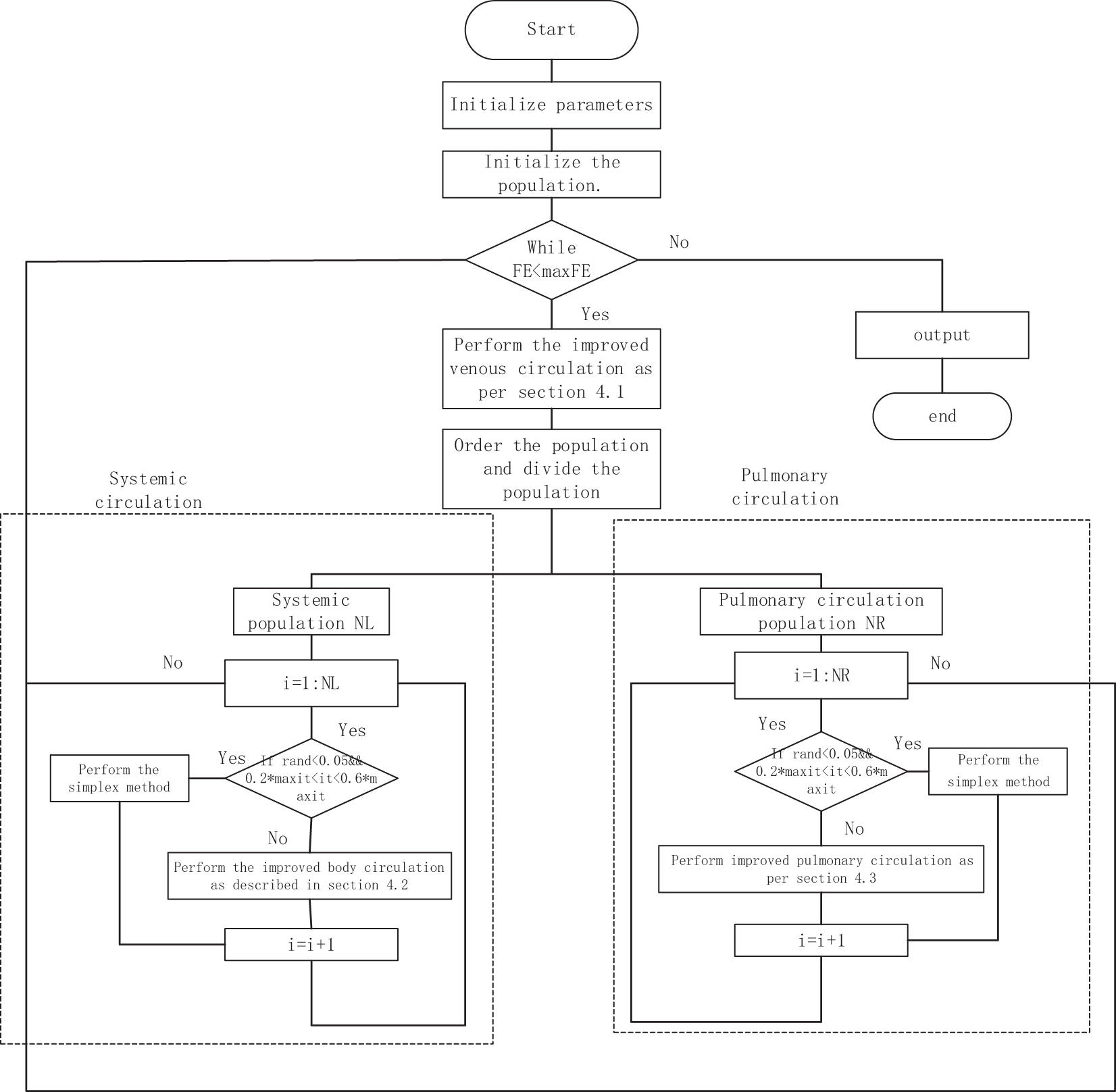
Figure 1: Flowchart of ICSBO algorithm

4.1 Improved Venous Circulation

As shown in Eq. (1) of Section 3.1, in the venous circulation phase of CSBO, the update of individuals relies on “self-learning of the individual + mutual learning between the individual and other individuals + perturbation learning between two random individuals.” Mutual learning and perturbation learning allow the gene information of the three random individuals to flow into the current individual, which helps maintain population diversity. However, the step size before mutual learning and perturbation learning is determined by Km,n × pi. According to Eq. (2), when individual Xpopm performs better than Xpopn, Km,n = +1; conversely, when individual Xpopm performs worse than Xpopn, Km,n = −1. Thus, Km,n only determines the direction of mutual learning and perturbation learning, whereas pi determines the degree of learning from mutual learning and perturbation learning.

According to literature [24], learning in the direction of superior individuals enhances the likelihood of individuals moving toward better positions, which can partially improve the algorithm’s convergence speed. The parameter Km,n can effectively achieve this purpose. To ensure the overall evolutionary direction of the population, mutual learning should play a dominant guiding role in individual evolution. The learning degree of mutual learning and perturbation learning cannot be exactly the same. Therefore, the direction guidance parameter Km,n is retained before mutual learning and perturbation learning, and different learning degrees are assigned to mutual learning and perturbation learning. A new venous circulation operation is proposed, as defined in Eq. (6).

Xpopinew=Xpopi+Ki,1×pi×(Xpopi−Xpop1)+K2,3×f1×(Xpop3−Xpop2)(6)

The generation method for f1 follows LSHADE (Improving the Search Performance of SHADE (Success-History based Adaptive Differential Evolution) Using Linear Population Size Reduction), and it is produced according to Eq. (7). If the generated f1 value is not within the boundary [0, H1], it needs to be revised according to Eq. (8).

f1=randc(uf(h),R)(7)

f1={randc(uf(h),R)iff1<0H1iff1>H1(8)

Here, H1 and R have different values at different evolutionary stages. When it ≤0.4×maxit, H1 = 0.9 and R = 0.1; otherwise, H1 = 1.2 and R = 1. randc represents the Cauchy distribution, and uf(h) denotes a value randomly selected from a D-dimensional array uf. In general, setting D = 5 produces satisfactory results, and this value can be adjusted based on the specific problem at hand. Initially, all elements in uf are set to 0.5. As iterations proceed, the elements in uf are updated as follows: First, the individuals that are successfully retained after updating according to Eq. (6) are saved to the set sg, and the corresponding f1 values of these individuals are saved to the set sf. Because each individual has a different f1 value, sf can contain up to Np elements or be an empty set. Then, the weights corresponding to the successfully retained individuals are calculated using Eq. (9), and the Lemher mean value for all successfully retained individuals is computed using Eq. (10). Finally, the elements of uf are updated algebraically according to Eq. (11)

wgfi=∑j=1dim(NCig−(∑j=1dimNCig/dim))2/dim∑i∈sf∑j=1dim(NCig−(∑j=1dimNCig/dim))2/dim(9)

Here, NCi represents the i-th individual in the set sg.

meanlf=∑i=1|sf|wgfi×sfi2∑i=1|sf|wgfi×sfi(10)

uf(t_f)={meanlfifsf≠∅0.5otherwise(11)

Here, t_f=(it−1)%5+1

In summary, compared with the original venous circulation operation shown in Eq. (1), the novel venous circulation operation proposed in this section uses the Cauchy distribution to determine the learning degree of perturbation learning. The mathematical formulation of the Cauchy distribution suggests that during the initial phases of evolution, the learning intensity of perturbation learning varies within the range [0, 0.9], and smaller scale parameters result in values clustered around 0.5. During the final phases of evolution, the learning degree of perturbation learning ranges from [0, 1.2], and larger scale parameters make values around 0.5 slightly more probable than other values. According to the generation method of Pi in Section 3.1, for better individuals, Pi is a normalized fitness value, whereas for poorer individuals, Pi is randomly generated within [0, 1]. Thus, better individuals are more likely to have Pi values greater than 0.5, whereas poorer individuals are more likely to have Pi values less than 0.5. Consequently, in the early stages of evolution, better individuals are more likely to have a learning degree of mutual learning greater than that of perturbation learning, which speeds up the convergence of better individuals. Conversely, for poorer individuals, the learning degree of mutual learning is more likely to be less than that of perturbation learning, which accelerates their shift toward other individuals and thus enhances the evolutionary speed while maintaining population diversity. During the final phases of evolution, the learning degree of perturbation learning is further increased compared with mutual learning, which better maintains the diversity of the population.

4.2 Improved Body Circulation Strategy

A thorough analysis of the systemic circulation strategy proposed by CSBO reveals that its convergence speed is slow, primarily due to the following reasons: First, intermediate individuals are generated through mutual learning among three randomly selected individuals from the venous blood population. While this random selection method helps maintain population diversity, the inherent randomness inevitably slows down the algorithm’s convergence speed. Second, when generating new individuals through crossover operations between intermediate individuals and original individuals, a high crossover probability results in the incorporation of only a small amount of gene information from the intermediate individuals into the original individuals. While this approach effectively maintains the existing diversity within the population, it considerably slows down the pace of population evolution.

To achieve an effective balance between convergence speed and population diversity, this section presents an improvement strategy for updating individuals in the elite population. Specifically, when the condition rand<0.05&0.2×maxit<it<0.6×maxit is satisfied, a new individual is created using the simplex method described in Section 4.2.1; otherwise, the approach outlined in Section 4.2.2 is used to generate a new individual. As with the systemic circulation strategy in CSBO, the top-performing individuals, whether newly generated or from the previous population, are selected for further evolution.

4.2.1 Simplex Method

The method for generating new individuals using the simplex method is as follows: Calculate the reflection point Xr of individual Xpopi using Eq. (12). If the fitness value at the reflection point fitr is greater than that of the current best individual Xgbest, generate a new individual using the expansion operation shown in Eq. (13). If the fitness value fitr is worse than that of individual Xpopi, generate a new individual using the contraction operation shown in Eq. (14). If Xr is worse than that of the current best individual Xgbest but better than Xpopi, generate a new individual using the shrinking operation shown in Eq. (15).

Xc=Xgbest+Xcibest2+b×(Xgbest+Xcibest2−Xpopi)(12)

Here, b is the reflection coefficient, typically set to 1; Xgbest and Xcibest denote the best and second-best values within the current population, respectively.

Xpopinew=Xc+λ×(Xr−Xc)(13)

Xpopinew=Xc+η×(Xpopi−Xc)(14)

Xpopinew=Xc−μ×(Xpopi−Xc)(15)

Here, λ is the expansion coefficient, typically set to 2; η is the compression coefficient, generally set to 0.5; and μ is the shrinking coefficient, generally set to 0.5. Xc=Xgbest+Xcibest2.

4.2.2 Novel Update Mechanism

The new individual update mechanism is as follows: First, similar to the generation method of f1 in Section 4.1, use the crossover probability cr as shown in Eq. (16). Then, generate intermediate individuals according to Eq. (17). Finally, perform crossover operations between intermediate individuals and original individuals dimension by dimension with the probability cr to generate new individuals.

cr=randc(ucr(h),R)(16)

The setting for R is exactly the same as in Section 3.1, and the update method for ucr(h) is similar to that in Section 4.1. It is important to note that when it≤0.4×maxit, if the generated cr is less than 0.5, a new cr is generated according to Eq. (16); if the generated cr is greater than 0.9, cr is directly set to 0.9. When it >0.4 maxit, if the generated cr is less than 0, a new cr is generated according to Eq. (16); if the generated cr is greater than 0.8, cr is directly set to 0.9.

Xpop_nlinew={Xpop_nli+pi×(Xpop_nli−Xpop1)+2×rand(1,dim)×(Xpop2−Xpop3)ifrand<tfpbest+pi×(gbest−Xpop1)else(17)

Here, Xpop1, Xpop2 and Xpop3 denote three randomly selected individuals from the population Xpop; pbest represents one individual randomly chosen from the top 3 best-performing individuals; gbest represents the optimal individual in the current population, tf is as shown in Eq. (18).

tf=eit−maxitmaxit(18)

In conclusion, the novel systemic circulation strategy introduced in this section offers several advantages. First, compared to the update mechanism in Section 3.2, the proposed strategy incorporates an exploration method based on the simplex approach, applied near the global optimal individual to generate new candidates. This method significantly improves the algorithm’s convergence speed. Moreover, the low frequency of simplex method execution helps preserve population diversity without causing excessive disruption. Additionally, the simplex method is only employed during the mid-evolution phase, ensuring global search during the early stages and reducing the risk of the algorithm getting trapped in local optima due to insufficient diversity in later stages. Second, as shown in Eq. (17), besides the simplex method, this section introduces two other search strategies: one executed when rand < tf, which maintains population diversity through sufficient interaction among individuals, and another improves convergence speed through learning from better and optimal individuals. In Eq. (18), tf gradually increases to 1 during the evolution. In the early evolution stage, this enhances convergence speed, whereas in the later stage, this better maintains population diversity. Third, the cr generation method proposed in this section varies with the evolution stage. In the early evolution stage, cr ranges from [0.5, 0.9], whereas in the later stage, it ranges from [0, 0.8]. Compared with the originally fixed higher cr values in CSBO, the cr values generated in this section are smaller in the early and later stages of evolution. This approach allows more gene flow into new individuals, which overall benefits the rapid convergence of the population. Additionally, the larger cr value range in the early evolution stage, combined with the crossover and search strategies, ensures improved convergence speed while maintaining a certain level of global search.

4.3 Improvements in the Pulmonary Circulation Stage

In Eq. (5), the update of individuals in the pulmonary circulation involves making slight perturbations to the original individuals to provide more diversity to the population. However, due to the randomness of the perturbations, the probability that the new individual is better than the original is extremely low. New individuals are rarely preserved for subsequent evolution, which leads to ineffective search, which not only hinders providing more population diversity but also reduces the algorithm’s convergence speed.

This section introduces an enhanced pulmonary circulation strategy to balance the convergence rate and population diversity: For each individual participating in the pulmonary circulation, if rand<0.05&0.2×maxit<it<0.6×maxit, a new individual is generated using the simplex method as described in Section 4.2.1; otherwise, a new individual is generated according to Eq. (19). As with the systemic circulation strategy in CSBO, the individual with the higher fitness, regardless of whether it is new or old, is selected to proceed to the next stage of evolution.

Xpop_nrinew={Xpopa2+rand×(Xpopb2−Xpopc2)+f2×(Xpopa2−Xpop_nri)ifrand>cr1Xduiliotherwise(19)

Here, Xpopb2 and Xpopc2 denote one individual randomly chosen from the top 10 best-performing and the 10 worst-performing individuals, respectively; Xpopa2 is an individual randomly chosen from the remaining individuals; f2 is a number generated using Lévy flight; cr1 is typically set to 1/3 for better results, but it can be manually adjusted based on the specific problem; Xduili represents the individual generated according to Eq. (20).

Xduili1,j={maxweij+minweij−Xpop_nrijifrand>cr2Xpop_nrijotherwise(20)

Here, maxweij and minweij denote the highest and lowest values of each dimension in the current population, respectively; Xpop_nrij′=maxweij+minweij−Xpop_nrij represents the opposition position of the current individual in dimension j; cr2 is a parameter, typically set to 0.1 for better results, but it can be manually adjusted based on the specific problem.

In summary, the newly proposed pulmonary circulation strategy in this section offers the following advantages: First, Eq. (20) provides two types of search modes. Mode one facilitates interaction among individuals from different regions. Mode two introduces opposition positions in certain dimensions. These two modes explore more of the search space in diverse ways and provide greater diversity to the population. Second, similar to Section 4.2, the combination of Eq. (20) with the simplex method improves the algorithm’s convergence speed while maintaining population diversity. Additionally, the three methods for generating individuals further enhance the algorithm’s success rate in solving different optimization problems.

4.4 Diversity Supplementation Mechanism Based on External Archives

Similar to other MHAs, CSBO can encounter situations where although the overall population diversity is acceptable, distinct individuals do not change across multiple generations during the solving of complex optimization problems. In such cases, these individuals contribute almost nothing to the evolution of the current population. To improve the optimization results and avoid wasting computational resources, this section establishes an external archive for each individual and designs the following diversity supplementation mechanism based on external archives:

Initially, individuals are directly stored in their respective archives. In subsequent iterations, If the newly generated individual outperforms the original one and its fitness is different from all individuals in the external archive, this new individual is added to the external archive. To prevent the archive from becoming extremely large, every k iteration, checks if the number of individuals exceeds a threshold gd, if it does, gd individuals are randomly chosen from the archive to create a new one. Generally, gd=5 and K=10 can yield satisfactory results, and they can also be modified according to the specific optimization problem. If an individual has not been updated for kt generations, it is replaced with a randomly selected individual from its corresponding archive to participate in subsequent evolution. Typically, kt=40 can achieve satisfactory results, but it can also be set according to specific needs.

4.5 Complexity Analysis

Assume that the population size of the ICSBO algorithm is N; the individuals in the part of body circulation and the part of pulmonary circulation are nl and nr, respectively, and the problem dimension is D. The problem dimension of the ICSBO algorithm is D.

The CSBO algorithm consists of the following three strategies: venous blood circulation, body circulation and pulmonary circulation. The maximum time complexity for a single run of the algorithm is as follows: 6N multiplications and 6N additions for venous circulation, 2nl multiplications and 4nl additions for somatic circulation, and 2nr multiplications and nr additions for pulmonary circulation. The worst time complexity of the CSBO algorithm is about 8 × O(N × D) + 8 × O(N).

The ICSBO algorithm consists of the following four main strategies: venous blood circulation, body circulation, pulmonary circulation, and external file. In the ICSBO algorithm running generation, the worst time complexity of the above links is as follows: The maximum time complexity for a single run of the algorithm is as follows: venous blood circulation needs to calculate a total of 6N multiplications and 6N additions; the body circulation needs to calculate a total of 4nl multiplications and 5nl additions; the lung circulation needs to calculate a total of 3nr multiplications and 5nr additions, and the external archive needs to calculate a total of 4N additions in a single iteration. additions. The worst time complexity of ICSBO is about 10 × O(N × D) + 14 × O(N).

5  Experimental Results and Analysis

The performance of the ICSBO algorithm will be assessed through the following experiments: (1) analyzing the sensitivity of the ICSBO algorithm’s parameters; (2) evaluating the impact of the four proposed enhancement strategies; (3) comparing the ICSBO algorithm’s performance with that of the original CSBO algorithm and eight other representative high-performance evolutionary algorithms in both 30-dimensional and 100-dimensional spaces; (4) conducting comparative experiments between the ICSBO algorithm and the top three algorithms from the comparison set on cooperative beam optimization problems to verify the proposed algorithm’s reliability.

For the experiments, the CEC2017 test suite which includes 30 benchmark functions, will be used. Functions F1 to F3 are unimodal, with F2 excluded due to its non-applicability for testing. Functions F4 to F10 are multimodal with local minima, F11 to F20 are mixed functions created by combining three or more CEC2017 benchmark functions via rotation or translation, and F20 to F29 are composite functions formed by combining at least three mixed functions or CEC2017 benchmark functions with rotation and translation. For further details on the CEC2017 test suite, refer to the provided documentation.

To maintain fairness in the comparison of algorithms, all experiments are conducted on a computer equipped with Windows 11, an Intel(R) Core(TM) i5-11400H @ 2.70 GHz CPU, and MATLAB R2021a for programming.

5.1 Parameter Sensitivity Testing

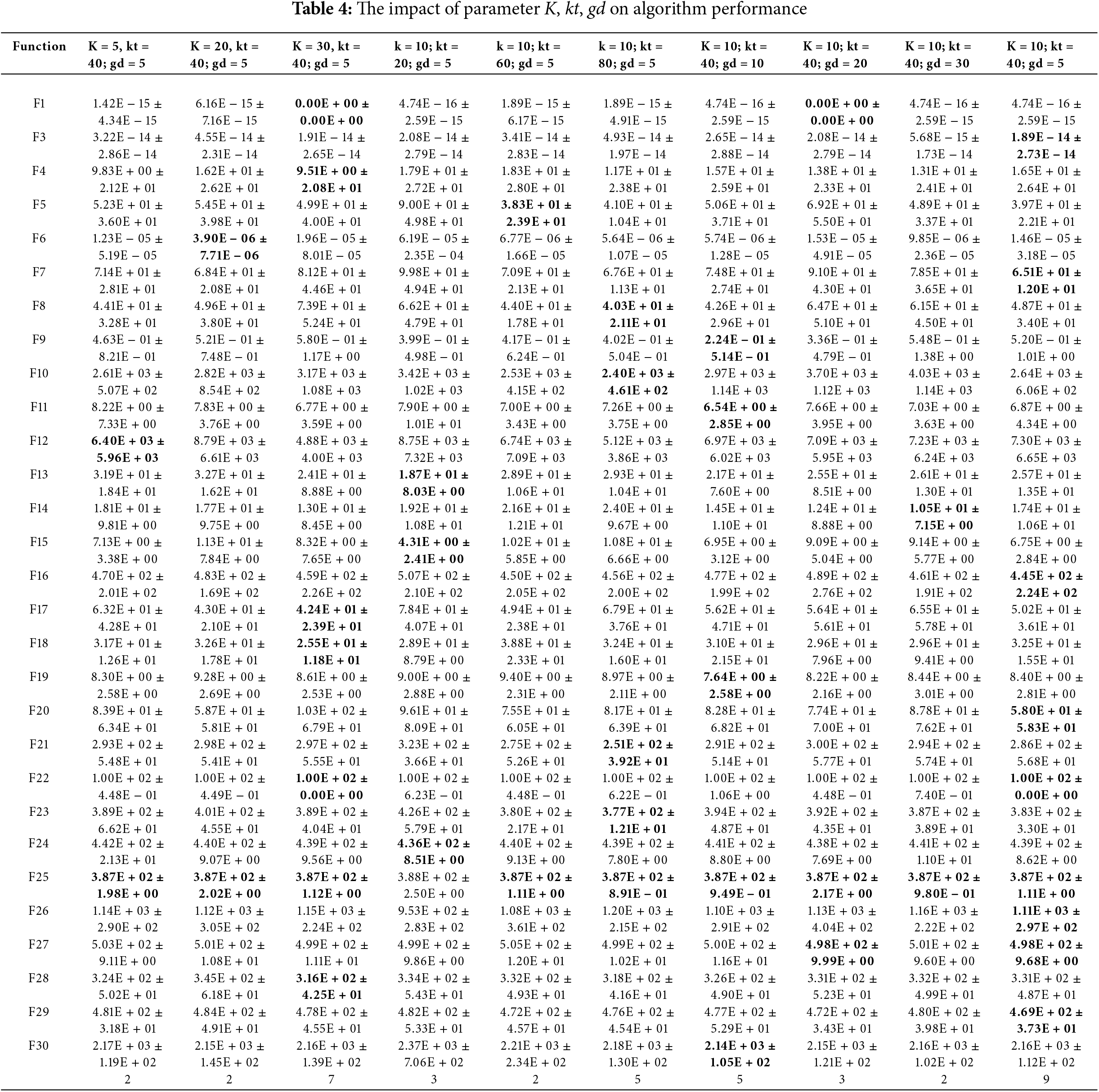
The ICSBO algorithm enhances the CSBO algorithm by introducing the following additional parameters: f1, cr, cr1, cr2, K, kt, and gd. Among these, f1 and cr use an adaptive update mechanism with restricted value ranges, while the remaining parameters are directly assigned values for participation in the algorithm’s iterative process. An experiment was conducted to examine how these parameters affect the performance of the ICSBO algorithm: in each trial, only one parameter’s value or range is modified, ensuring that other parameters of the algorithm remain unchanged. Each algorithm’s population size is set to N = 50, with a test function dimensionality of D = 30 and a maximum function evaluation count of MaxFEs = 300,000. Other parameters are set as follows: maxit = 3000, kt = 40, gd = 5, K = 10. To avoid the randomness of single-run operations, each algorithm is executed 30 times independently on each test function, with the mean and variance recorded; specific data are shown in Tables 1 to 4. The parameter settings for each trial are as follows:

(1) To assess the impact of the parameter f1 on the algorithm’s performance, two sets of experiments were conducted. In the first set, when it ≤0.4 × maxit, the parameter values are chosen from the following three groups, [0, 0.3] [0.3, 0.6] [0.6, 0.9]; it >0.4 × maxit, the range of values of f1 is dimensioned as [0, 1.2], and the second group: for it >0.4 × maxit, the range of values is taken as [0, 0.4] [0.4, 0.8] [0.8, 1.2], and the second group: when it >0.4 × maxit, the range of values is taken as [0, 0.4] [0.4, 0.8] [0.8, 1.2]. The second group: when it >0.4 × maxit, the range of values is [0, 0.4] [0.4, 0.8] [0.8, 1.2]; when it ≤0.4 × maxit, the range of values of f1 is [0, 0.8]. The rest of the parameters of the two experiments are the same, and the values of each parameter are as follows: cr is [0.5, 0.9] for it ≤0.4 × maxit, [0, 0.8] for it >0.4 × maxit, 0.3 for cr1, 0.1 for cr2, 10 for k, 40 for kt, and 5 for gd;

(2) To investigate the impact of the parameter cr on the algorithm’s performance, two sets of experiments are conducted. When it ≤0.4 × maxit, the values of cr are selected from the following three ranges: [0.3, 0.5] [0.5, 0.7] [0.7, 0.9], and when it >0.4 × maxit, the range of cr is taken as [0, 0.8]; the second group of experiments: when it >0.4 × maxit, the range of cr is taken as [0, 0.3] [0.3, 0.6] [0.6, 0.8]; and the second group of experiments: when it >0.4 × maxit, the range of cr is taken as [0, 0.3] [0.3, 0.6] [0.6, 0.8]. The second set of experiments: when it >0.4 × maxit, the value range of cr is [0, 0.3] [0.3, 0.6] [0.6, 0.8]; when it ≤0.4 × maxit, the value range of f1 is [0.5, 0.9]. The rest of the parameters of the two experiments are the same, and the values of each parameter are as follows: f1 is [0, 0.8] for it ≤0.4 × maxit, [0, 1.2] for it >0.4 × maxit, 0.3 for cr1, 0.1 for cr2, 10 for k, 40 for kt, and 5 for gd;

(3) To examine the impact of the parameters cr1 and cr2 on the algorithm’s performance, the following two sets of parameter values were used: 0.1, 0.6, and 0.9; 0.4, 0.7, and 1. Other than that, the other parameters were set as follows: f1 in the range of [0, 0.8] for it ≤0.4 × maxit, [0, 1.2] for it >0.4 × maxit, [0.5, 0.9] for it ≤0.4 × maxit, and [0, 0.5, 0.9] for it >0.4 × maxit, and [0, 0.5, 0.5] for it >0.4 × maxit, and [0, 0.5, 0.9] for it >0.4 × maxit. maxit and [0.5, 0.9] for it ≤0.4 × maxit, [0, 0.8] for it >0.4 × maxit, 10 for K, 40 for kt and 5 for gd;

(4) In examining the effect of the parameter K, kt, and gd on the performance of the algorithm, the following three sets of parameters are: 5, 20 and 30; 20, 60 and 80; and 10, 20 and 30. Other than that, the other parameters were set as follows: f1 in the range of [0, 0.8] for it ≤0.4 × maxit, [0, 1.2] for it >0.4 × maxit, cr in the range of [0.5, 0.9] for it ≤0.4 × maxit, and [0.5, 0.9] for it >0.4 × maxit, and [0.5, 0.9] for it >0.4 × maxit, and [0.5, 0.9] for it >0.4 × maxit. 0.5, 0.9] for it ≤0.4 × maxit, [0, 0.8] for it >0.4 × maxit, 0.3 for cr1 and 0.1 for cr2.

As presented in Tables 1 to 4, the last row shows how many times the algorithm achieved the global optimum across all functions. From the Tables, it is evident that, unless specified otherwise, f1 takes the value range of [0, 0.8] for it ≤0.4 × maxit, [0.1.2] for it >0.4 × maxit, cr takes the value range of [0.5, 0.9] for it ≤0.4 × maxit, [0, 0.8] for it >0.4 × maxit, and cr1 takes the value of 0.5, 0.9, 0.8, and cr1 takes the value of 0.5, 0.9 for it >0.4 × maxit, and cr1 takes the value of 0.0, 0.8. The algorithm achieves better optimization performance when cr1 is taken as 0.3, cr2 is taken as 0.1, K is taken as 10, kt is taken as 40 and gd is taken as 5.

5.2 Effectiveness Experiments of Various Improvement Strategies

According to Section 4, the ICSBO algorithm introduces four improvements to the CSBO algorithm. To verify the effectiveness of these four improvement strategies, we created four new modified algorithms by removing each corresponding improvement strategy from ICSBO and replacing it with the corresponding strategy from the basic CSBO algorithm. These include: (1) removing the improved venous blood circulation strategy from Section 4.1, (2) removing the improved body circulation strategy from Section 4.2, (3) removing the improved lung circulation strategy from Section 4.3, and (4) removing the external archive-based diversity supplementation mechanism from Section 4.4. For simplicity, these four new modified algorithms are named ICSBO1, ICSBO2, ICSBO3, and ICSBO4, and are compared with the ICSBO algorithm on the CEC2017 test suite.

To ensure a fair comparison, each algorithm is tested with a population size of N = 50, a dimension of D = 30, and a maximum of MaxFEs = 300,000 function evaluations. The additional parameters are set as follows: maxit = 3000 kt = 5, gd = 5, and K = 10. To mitigate the effects of randomness from a single run, each algorithm is run independently 30 times on each test function.

Table 5 displays the results of the algorithms over 29 test functions, with the “±” symbol representing the mean and standard deviation of the optimal values from 30 independent runs. To further compare the performance of the ICSBO algorithm with other improved algorithms, Wilcoxon rank-sum and Friedman tests were performed at a 5% significance level, as shown in Tables 6 and 7. In Table 6, a p-value greater than 0.05 indicates no significant difference between the ICSBO algorithm and the respective improved algorithm, marked by the symbol “=”. A p-value less than 0.05, with the improved algorithm showing a better average optimal value from 30 runs, indicates that the improved algorithm significantly outperforms the ICSBO, represented by the symbol “+”. Conversely, if the performance is significantly worse, it is indicated by the symbol “−”. In Table 7, a lower rank mean for an algorithm signifies better overall performance.

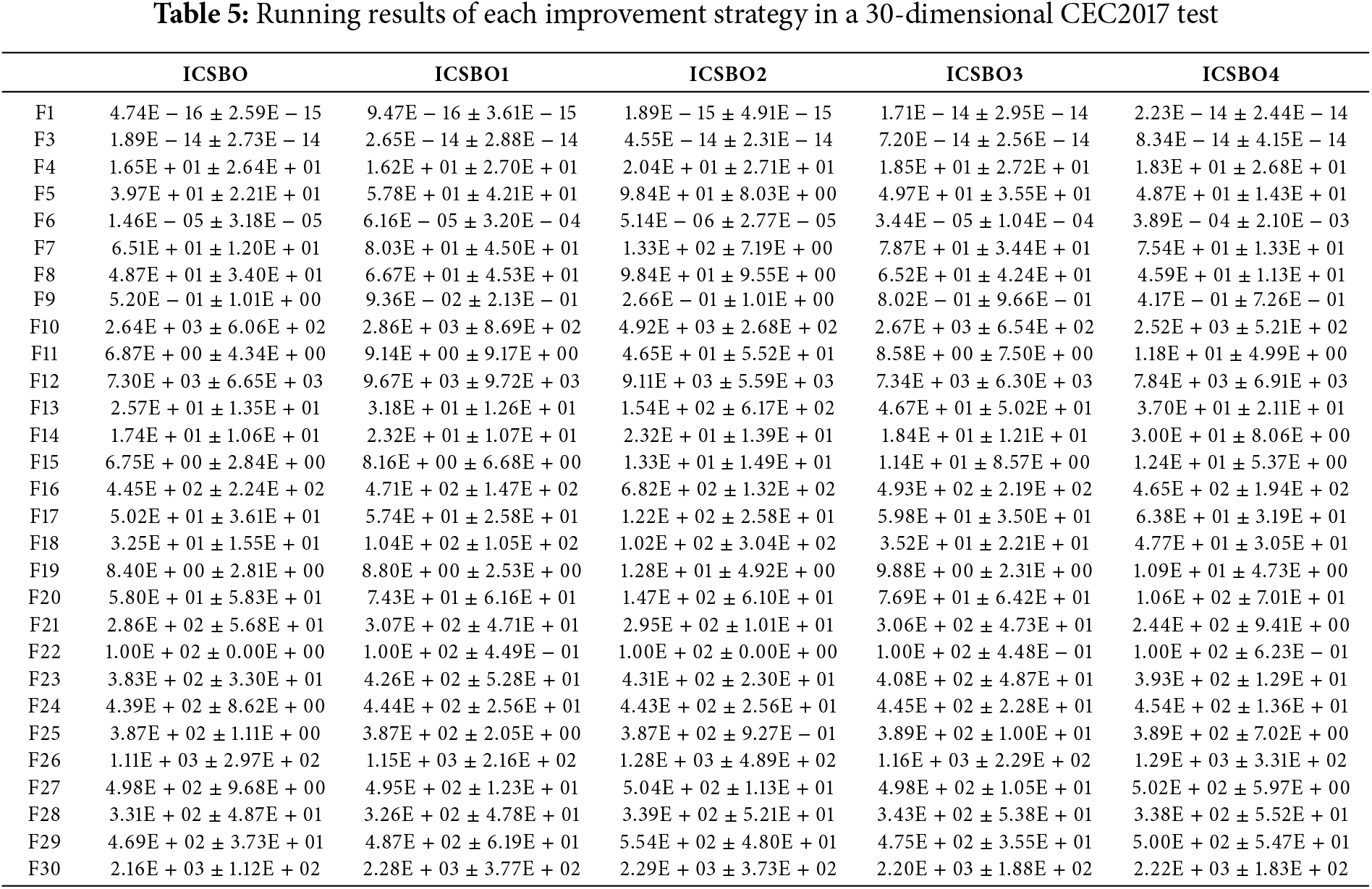
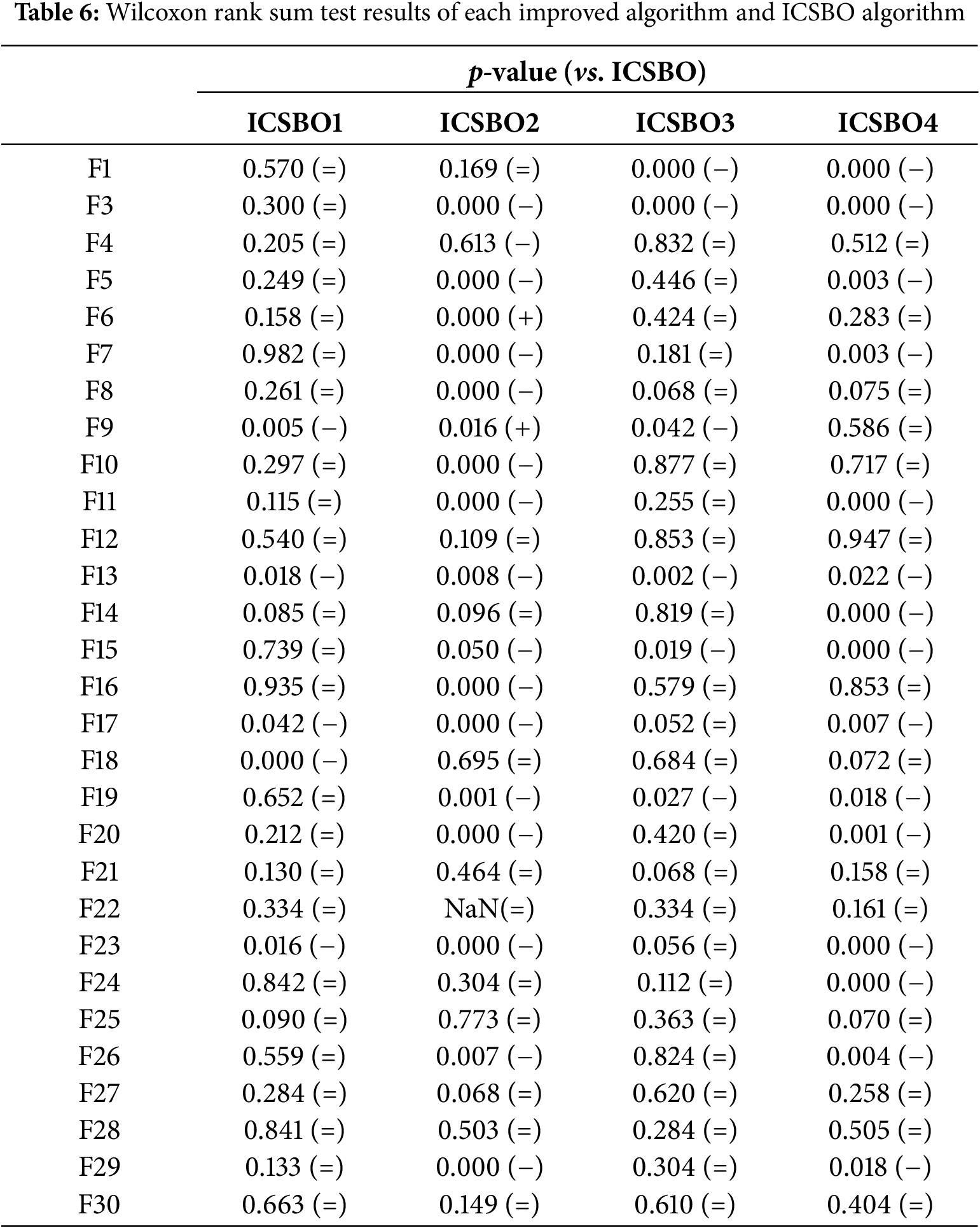
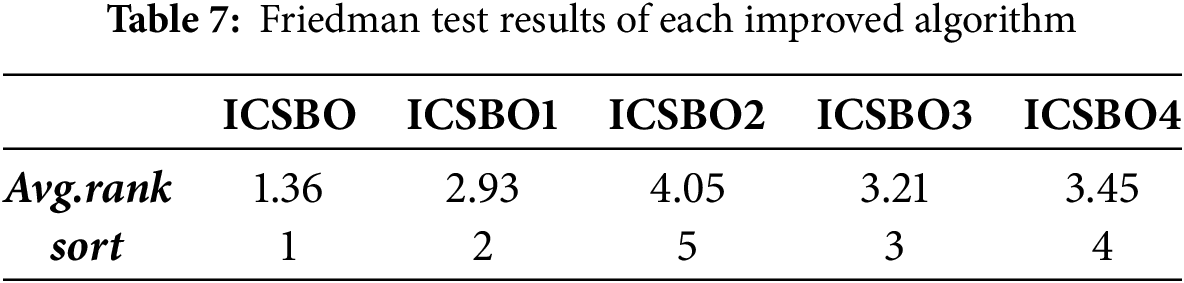
Table 5 shows that, compared to the ICSBO algorithm, the performance of the four improved algorithms is worse than that of ICSBO in 25, 26, 26, and 25 test functions, respectively. According to the Wilcoxon rank-sum test results in Table 6, ICSBO1 performs worse than ICSBO in 5 test functions, marked by a “ − ”, while in the remaining 24 functions, the performance is comparable, indicated by “=”. ICSBO2 outperforms ICSBO in 2 test functions, has similar performance in 11, and underperforms in 16. ICSBO3 shows similar performance to ICSBO in 23 test functions and worse performance in 6. ICSBO4 performs similarly to ICSBO in 14 functions and worse in 15. Table 7 shows that excluding any of the improvement strategies from ICSBO results in a decline in the rankings of the modified algorithms, indicating that the four proposed strategies have a significant impact on the overall performance of ICSBO.

In conclusion, the four improvement strategies introduced in this paper show varying degrees of effectiveness. The strategies outlined in Sections 4.2 and 4.4 have a more significant impact on the performance of ICSBO, while the performance improvements from the other two strategies are similar to that of the original ICSBO.

5.3 Comparison of ICSBO Algorithm Performance with Other Algorithms

To evaluate whether the ICSBO algorithm outperforms others in convergence accuracy and speed, this section compares its performance with eight representative evolutionary algorithms using the CEC2017 test suite. These algorithms include the Enhanced Serpent Optimizer (ESO), which introduces a new dynamic mechanism and an opposition-based learning strategy; the Improved Orca Predation Algorithm (IOPA); the Improved Archimedes Algorithm (IAOA); the Multi-Strategy Enhanced CSBO (MECSBO) algorithm; the Strategy-Enhanced MDBO algorithm; the Multi-Trial Vector Sine Cosine Algorithm (MTV-SCA); the newly proposed Synergistic Swarm Optimization Algorithm (SSOA); and the Information Acquisition Optimization Algorithm. To ensure fairness in comparison, all algorithms will use a population size of N = 50 and a maximum function evaluation count of MaxFEs = 300,000. Table 8 presents the parameter settings for each algorithm, with the values for the comparison algorithms matching those used in the original studies.

5.3.1 Comparison of Convergence Accuracy between the ICSBO Algorithm and Other Algorithms

To assess the convergence accuracy of the ICSBO algorithm relative to other algorithms, experiments were conducted using the CEC2017 test suite with D = 30. Table 9 displays the average values and standard deviations for each algorithm, based on 30 independent runs in 30 dimensions of the CEC2017 dataset, with the best optimization results highlighted in bold. The table also presents the outcomes of the Wilcoxon rank-sum test, comparing the ICSBO algorithm with the other algorithms. For a more thorough evaluation of the overall performance, Table 10 provides the results from the Friedman test.

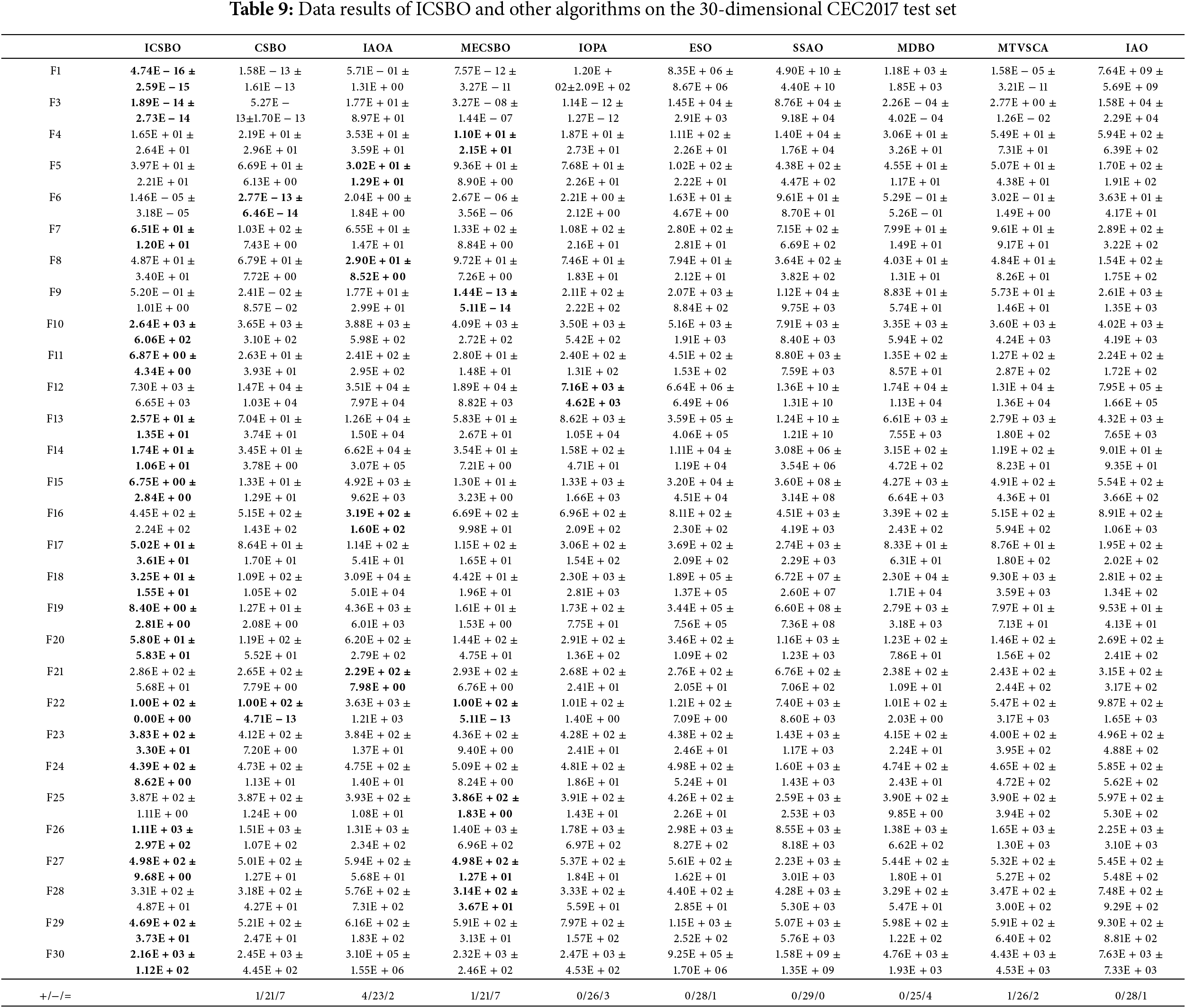
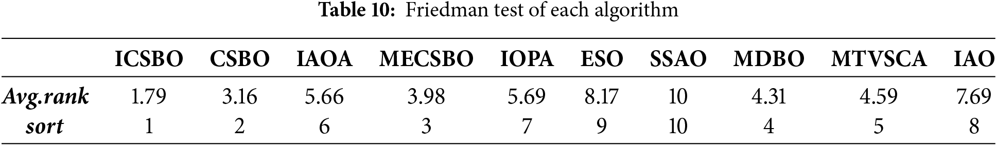
Table 9 shows that in 30-dimensional optimization problem, ICSBO achieves global optimality in 18 test functions, including F1, F3, F7, F10, F11, F13, F14, F15, F17, F18, F19, F20, F22, F23, F24, F27, F29, F30; CSBO attains global optimality in 2 functions, including F6, F22; MECSBO obtains global optimum in 6 functions including F4, F9, F22, F25, F27, F28; IAOA achieves global optimum in 6 functions, including F5, F8, F13, F16, F18, F21; IOPA attains global optimum in F12, and MDBO achieves global optimum in F25. The optimization results in Table 10 show that compared with ICSBO, CSBO performs similarly in 7 functions, worse in 21 functions, and better in 1 function; MECSBO performs similarly in 7 functions, worse in 21 functions, and better in 1 function; IAOA has only 2 functions, and the 4 remaining functions have the same performance. Performance is equal, the 4 remaining functions have better performance, and 23 functions have worse performance. MTV-SCA has worse performance in 26 functions, a slightly different performance in 2 functions, and better performance in 1 function. IOPA has equal performance in 3 functions and worse performance in the 26 remaining functions. MDBO has equal performance in 5 functions and worse performance on 24 functions compared with ICSBO. ESO and IAO have 28 functions with worse performance and only 1 function with flat performance. SSOA performs worse than ICSBO in 29 functions. Table 10 illustrates that, for the 30-dimensional test functions, the ranking order is ICSBO > CSBO > MECSBO > MDBO > MTV-SCA > IAOA > IOPA > IAO > ESO > SSOA. In conclusion, the ICSBO algorithm demonstrated a significant enhancement in convergence accuracy compared to other algorithms on the 30-dimensional CEC2017 test suite.

Table 11 presents the mean and standard deviation of the algorithms from 30 independent experiments conducted on the 100-dimensional CEC2017 dataset, along with the results of the Wilcoxon rank-sum test. The function that achieves the best optimization result for each case is highlighted in bold.

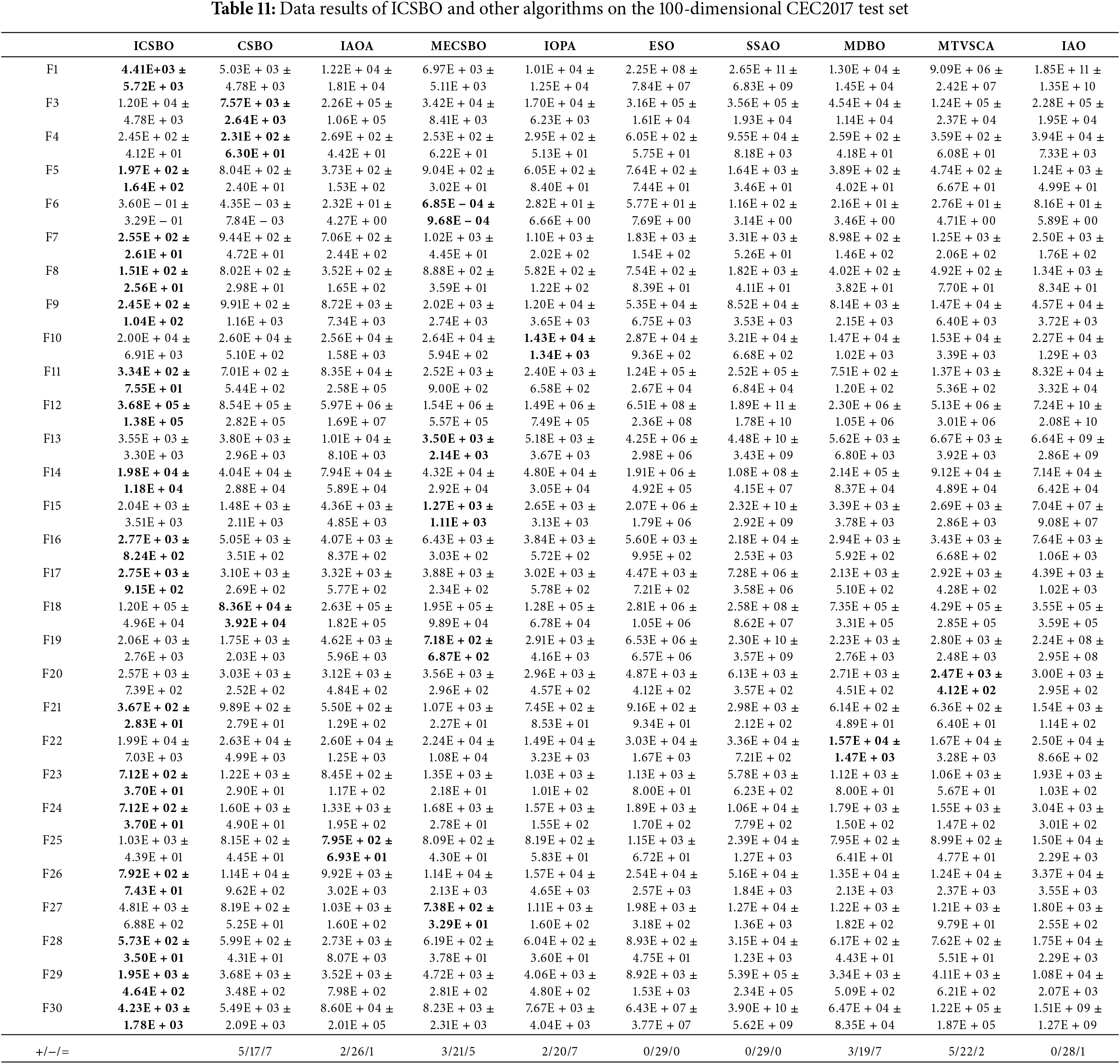
Table 11 shows that ICSBO can take the global optimum in 17 functions such as F1, F5, F7, F9, F11, F12, F14 F16, F17, F21, F23, F24, F26, F28, F29, F30, CSBO can take the global optimum in 3 functions such as F3, F4, F18, MECSBO can take the global optimum in F6, F13, F15, F18, F26, MTVSCA can take the function optimum in F20, F22, IAOA can take the global optimum in F25, and IOPA can take the global optimum in F10. Compared with ICSBO, IAOA performs better in 2 functions, worse in 26 functions, and equally in 1 function. MECSBO outperforms ICSBO in 3 functions, worse in 21 functions, and performs equally in five functions. IOPA outperforms ICSBO in 2 functions, worse in 20 functions, and performs equally in 7 functions. ESO and SSOA are worse than ICSBO. IAO is worse than ICSBO in 28 functions and performs equally in only 1 function. MDBO outperforms ICSBO on 3 functions, worse in 19 functions, and performs equally on 5 functions. The MDBO algorithm outperforms the ICSBO algorithm in 3 functions, worse in 19 functions, and is equal in 7 functions. MTVSCA outperforms ICSBO in 5 functions, worse in 22 functions, and performs equally in 2 functions.

Tables 9 and 11 show that as the dimensionality increases, the algorithm’s performance changes, with the impact on single-peak functions being particularly pronounced. The ICSBO algorithm proposed in this paper performs well in 100 dimensions, achieving the global optimum for nearly 17 functions. When compared to the results from the 30-dimensional tests on multi-peak, composite, and combined functions, ICSBO’s performance remains stable. This consistency further demonstrates that ICSBO maintains good convergence accuracy and faster convergence speed.

5.3.2 Comparison of Convergence Speed between the ICSBO Algorithm and Other Algorithms

Fig. 2 provides a visual comparison of the convergence speeds for each algorithm, displaying the convergence curves across the 29 test functions in the 30-dimensional CEC2017 test suite. The x-axis represents the number of evaluations, while the y-axis displays the logarithmic values of the fitness scores. (The subscripts of each picture in Fig. 2 indicate the tested function, and because the F2 function is not tested, it is not shown).

Figure 2: Convergence curves of 29 functions on CEC2017 test set between ICSBO algorithm and other 8 comparison algorithms (The different algorithms represented by the different color curves are shown in the final figure F31)

Fig. 2 reveals that in unimodal functions (F1 and F3), ICSBO achieves the optimal value and the fastest convergence speed. Specifically, in F1, ICSBO substantially accelerates during the middle stages of evolution compared with the other algorithms and stabilizes in the later stages until reaching the optimal value. In F3, ICSBO exhibits a clear advantage during the early and middle stages of evolution, and is second only to IAOA. In multimodal functions (F4–F10), as shown in Fig. 2, ICSBO exhibits a noticeable advantage in convergence speed in F6 and F9. In F4, the convergence speed of ICSBO is comparable with that of other algorithms in the early stages, but its performance is inferior to that of IOPA, MDBO, CSBO, and MECSBO in the later stages. In F5 and F8, ICSBO accelerates during the middle stages, with smooth convergence in the early and later stages. In F5, the performance of ICSBO is close to that of MDBO but inferior to that of IAOA. In F8, the performance of ICSBO is similar to that of MDBO and MECSBO but behind that of MECSBO. In F7, ICSBO speeds up during the middle stages and stabilizes later on; it performs similarly to IOPA and MDBO and outperforms other algorithms. In F10, the performance of ICSBO is comparable with that of other algorithms in the early and middle stages but accelerates in the later stages, although its overall performance is still inferior to that of MDBO. In hybrid functions (F11–F20), as shown in Fig. 2, ICSBO achieves the global optimum and demonstrates satisfactory convergence speed in functions F11, F12, F14–F17, and F19. In F13, F18, the convergence speed of ICSBO is similar to that of MECSBO and CSBO. In F20, ICSBO accelerates its convergence speed in the early and middle stages, and levels off its speed in the later stages; it performs similarly to MTVSCA but is overall slightly inferior to MTVSCA. In composite functions (F21–F30), ICSBO achieves the global optimum in functions F24, F28, and F29. In functions F22, F23, F25, F27, and F30, the convergence speed and accuracy of ICSBO are comparable with those of CSBO, MECSBO, IAOA, and MDBO. However, in F21, ICSBO performs poorly; only outperforms SSOA, ESO, and IAO; and performs worse than the five other algorithms. In F26, ICSBO performs worse than MDBO but better than the other algorithms. In summary, compared with the eight other algorithms, ICSBO shows a certain advantage in convergence speed.

5.4 Comparison of Engineering Application Effects

To further evaluate the effectiveness of ICSBO in engineering applications, this section investigates its performance on the cooperative beamforming optimization problem. This problem, commonly encountered in antenna arrays, involves optimizing the amplitude (ξ∈[0,1]) and phase (α∈[−π,π]) of the transmit signal weights at each cooperative node. These parameters are considered as decision variables during the optimization process, with the goal of minimizing the PSL (peak sidelobe level), as specified in Eq. (21).

PSL=20log10⁡max|AF(θSL,w)|AF(φ,w)(21)

In this context, AF(θ,w) represents the array factor, as given in Eq. (22). The value φ corresponds to the direction of the main beam, while θSL indicates the direction of the side lobes in the array factor, excluding the main beam peaks, within the range of θ∈[−π,φ)∪(φ,π]. The denominator, AF(φ,w), refers to the power of the main beam, while the numerator, max|AF(θSL,w)|, represents the maximum power of the side lobes.

AF(θ,w)=∑k=1kwkej(2π/λ)rk[cos⁡(θ−ψk)](22)

In this study, the ICSBO algorithm is compared with MECSBO, MDBO, and MTVSCA algorithms on the cooperative beam optimization problem to assess its effec-tiveness. To ensure a fair comparison, the problem size (N) in this experiment is set to 20, with a maximum of 50 function evaluations (maxit = 50), 4 nodes (k = 4), a pole radius of 1 (r = 1), and a dimension of 2 k (dim = 2 k). Additional parameter settings for each algorithm are provided in Table 5. Fig. 3 presents the beam pattern of the ICSBO algorithm alongside the comparison algorithms in the Cartesian coordinate system, with the corresponding PSL values for each algorithm annotated within the figure.

Figure 3: Beamplot of ICSBO vs. other algorithms in the Cartesian coordinate system

As shown in Fig. 3, the ICSBO algorithm achieves an optimal PSL value of −15.1850 dB, while the MECSBO, MDBO, and MTVSCA algorithms yield values of −12.3975, −6.5643, and −13.0285 dB, respectively. Among these, ICSBO delivers the lowest PSL, demonstrating the best performance in cooperative beam optimization. Overall, the ICSBO algorithm exhibits outstanding effectiveness in engineering applications.

6  Conclusion

This paper proposes ICSBO, which further enhances the convergence speed and local optima escape capability of CSBO. Initially, corresponding improvement strategies are introduced for the three components of CSBO: venous blood circulation, body circulation, and pulmonary circulation. These improvements enrich population diversity and reduce the likelihood of becoming trapped in local optima during evolution. By dividing the evolutionary process and improving the parameters and updating methods, the convergence speed of the population is accelerated in the early stages of evolution. Additionally, the introduction of the simplex method in the body and pulmonary circulation further speeds up convergence. Finally, to increase population diversity and reduce gene loss, an archive updating mechanism is designed to enhance the utilization probability of high-quality genes. The simulation results across multiple experiments on the CEC2017 benchmark set indicate that the proposed improvements significantly boost the overall performance of ICSBO, demonstrating significant improvements in both convergence rate and solution precision compared to other algorithms.

While the ICSBO algorithm presented in this paper offers significant benefits in convergence accuracy, its time complexity tends to rise. Future studies will aim to minimize the time complexity of ICSBO. Furthermore, the application of ICSBO in practical engineering problems will be explored in greater depth.

Acknowledgment: The authors would like to thank the anonymous reviewers and the editor for their valuable suggestions, which greatly contributed to the improved quality of this article.

Funding Statement: This work is partially supported by the Project of Scientific and Technological Innovation Development of Jilin in China under Grant 20210103090.

Author Contributions: The authors confirm contribution to the paper as follows: study conception and design: Yanjiao Wang, Zewei Nan; data collection: Zewei Nan; analysis and interpretation of results: Yanjiao Wang, Zewei Nan; draft manuscript preparation: Yanjiao Wang, Zewei Nan. All authors reviewed the results and approved the final version of the manuscript.

Availability of Data and Materials: The data that support the findings of this study are openly available at https://gitcode.com/open-source-toolkit/456e4 (accessed on 11 October 2024).

Ethics Approval: Not applicable.

Conflicts of Interest: The authors declare no conflicts of interest to report regarding the present study.

References

1. Ghasemi M, Akbari MA, Jun C, Bateni SM, Zare M, Zahedi A, et al. Circulatory System Based Optimization (CSBOan expert multilevel biologically inspired meta-heuristic algorithm. Eng Appl Comput Fluid Mech. 2022;16(1):1483–525. doi:10.1080/19942060.2022.2098826. [Google Scholar] [CrossRef]

2. Garg H. An efficient biogeography based optimization algorithm for solving reliability optimization problems. Swarm Evol Comput. 2015;24:1–10. doi:10.1016/j.swevo.2015.05.001. [Google Scholar] [CrossRef]

3. Karaboga D, Celal O. A novel clustering approach: Artificial Bee Colony (ABC) algorithm. Appl Soft Comput. 2011;11(1):652–7. doi:10.1016/j.asoc.2009.12.025. [Google Scholar] [CrossRef]

4. Mirjalili S, Mirjalili S. Genetic algorithm. Evol Algorithms Neural Netw: Theory Appl. 2019;780:43–55. doi:10.1007/978-3-319-93025-1_4. [Google Scholar] [CrossRef]

5. Mallipeddi R, Suganthan PN, Pan QK, Tasgetiren MF. Differential evolution algorithm with ensemble of parameters and mutation strategies. Appl Soft Comput. 2011;11(2):1679–96. doi:10.1016/j.asoc.2010.04.024. [Google Scholar] [CrossRef]

6. Cai X, Zhao H, Shang S, Zhou Y, Deng W, Chen H, et al. An improved quantum-inspired cooperative co-evolution algorithm with muli-strategy and its application. Expert Syst Appl. 2021;1(1):114629. doi:10.1016/j.eswa.2021.114629. [Google Scholar] [CrossRef]

7. Dorigo M, Birattari M, Stutzle T. Ant colony optimization. IEEE Comput Intell Mag. 2007;1(4):28–39. doi:10.1109/MCI.2006.329691. [Google Scholar] [CrossRef]

8. Mirjalili S, Mirjalili SM, Lewis A. Grey wolf optimizer. Adv Eng Softw. 2014;69:46–61. doi:10.1016/j.advengsoft.2013.12.007. [Google Scholar] [CrossRef]

9. Arora S, Singh S. Butterfly optimization algorithm: a novel approach for global optimization. Soft Comput. 2018;23:715–34. doi:10.1007/s00500-018-3102-4. [Google Scholar] [CrossRef]

10. Braik M, Hammouri A, Atwan J, Al-Betar MA, Awadallah MA. White shark optimizer: a novel bio-inspired meta-heuristic algorithm for global optimization problems. Knowl Based Syst. 2022;243:108457. doi:10.1016/j.knosys.2022.108457. [Google Scholar] [CrossRef]

11. Hashim FA, Hussain K, Houssein EH, Mabrouk MS, Al-Atabany W. Archimedes optimization algorithm: a new metaheuristic algorithm for solving optimization problems. Appl Intell. 2021;51:1531–51. doi:10.1007/s10489-020-01893-z. [Google Scholar] [CrossRef]

12. Rao RV, Savsani VJ, Vakharia DP. Teaching-learning-based optimization: a novel method for constrained mechanical design optimization problems. Comput-Aided Design. 2011;43(3):303–15. doi:10.1016/j.cad.2010.12.015. [Google Scholar] [CrossRef]

13. Mohamed AW, Hadi AA, Mohamed AK. Gaining-sharing knowledge based algorithm for solving optimization problems: a novel nature-inspired algorithm. Int J Mach Learn Cybern. 2020;11(7):1501–29. doi:10.1007/s13042-019-01053-x. [Google Scholar] [CrossRef]

14. Wu X, Li S, Jiang X, Zhou Y. Information acquisition optimizer: a new efficient algorithm for solving numerical and constrained engineering optimization problems. J Supercomput. 2024;80(18):25736–91. doi:10.1007/s11227-024-06384-3. [Google Scholar] [CrossRef]

15. Yao L, Yuan P, Tsai CY. ESO: an enhanced snake optimizer for real-world engineering problems. Expert Syst Appl. 2023;230:120594. doi:10.1016/j.eswa.2023.120594. [Google Scholar] [CrossRef]

16. Wang YJ, Chen MC, Ku CS. An improved archimedes optimization algorithm (IAOA). J Netw Intell. 2023;8(3):693–709. [Google Scholar]

17. Hu G, Wei G, Abbas M. Opposition-based learning boosted orca predation algorithm with dimension learning: a case study of multi-degree reduction for NURBS curves. J Comput Des Eng. 2023;10(2):722–57. doi:10.1093/jcde/qwad017. [Google Scholar] [CrossRef]

18. Ye M, Zhou H, Yang H, Hu B, Wang X. Multi-strategy improved dung beetle optimization algorithm and its applications. Biomimetics. 2024;9(5):291. doi:10.3390/biomimetics9050291. [Google Scholar] [PubMed] [CrossRef]

19. Nadimi-Shahraki MH, Taghian S, Javaheri D, Sadiq AS, Khodadadi N, Mirjalili S. MTV-SCA: multi-trial vector-based sine cosine algorithm. Cluster Comput. 2024;27:1–45. doi:10.1007/s10586-024-04602-4. [Google Scholar] [CrossRef]

20. Alzoubi S, Sharaf L, Sharaf M, Daoud MS, Khodadadi N, Jia H. Synergistic swarm optimization algorithm. CMES-Comput Model Eng Sci. 2024;139(3):2557–604. doi:10.32604/cmes.2023.045170. [Google Scholar] [CrossRef]

21. Abdollahzadeh B, Gharehchopogh FS, Khodadadi N, Mirjalili S. Mountain gazelle optimizer: a new nature-inspired metaheuristic algorithm for global optimization problems. Adv Eng Softw. 2022;174:103282. doi:10.1016/j.advengsoft.2022.103282. [Google Scholar] [CrossRef]

22. Yang S, Guo C, Meng D, Guo Y, Guo Y, Pan L, et al. MECSBO: multi-strategy enhanced circulatory system based optimisation algorithm for global optimisation and reliability-based design optimisation problems. IET Collab Intell Manuf. 2024;6(2):e12097. doi:10.1049/cim2.12097. [Google Scholar] [CrossRef]

23. Ji J, Wu T, Yang C. Neural population dynamics optimization algorithm: a novel brain-inspired meta-heuristic method. Knowl Based Syst. 2024;300:112194. doi:10.1016/j.knosys.2024.112194. [Google Scholar] [CrossRef]

24. Wang F, Zhang H, Li K, Lin Z, Yang J, Shen XL. A hybrid particle swarm optimization algorithm using adaptive learning strategy. Inf Sci. 2018;436:162–77. doi:10.1016/j.ins.2018.01.027. [Google Scholar] [CrossRef]