A Base Station Deployment Algorithm for Wireless Positioning Considering Dynamic Obstacles

1  Introduction

In security systems, the Radio Frequency Identification (RFID) positioning technology is mainly used to obtain the location information of personnel, staff utilize wearable positioning devices to receive wireless RF signals from RFID base stations. The fluctuating layout of obstacles and base stations within the positioning area notably impacts the strength of the RF signals. Swiftly computing a deployment plan to adapt to changes in the obstacle landscape is crucial for ensuring signal coverage within the system. Real-time monitoring of security personnel positions enhances the safety and reliability of the system.

In the realm of research focused on optimizing wireless base station deployment, many studies assume that deployment occurs in an obstacle-free environment where signals propagate without hindrance. However, obstacles are prevalent in practical scenarios, and their positions fluctuate. Neglecting obstacles when devising deployment strategies leads to an inevitable decline in signal transmission quality. Therefore, we must explore optimization strategies for base station deployment in dynamic, obstacle-laden environments.

Wu et al. [1] introduced a wireless sensor network (WSN) topology model that considers obstacles in a study exploring obstacle-aware sensing models. This model assumes that the perception probability between a signal transmitter and receiver is zero if obstacles obstruct the path. While this model effectively identifies barriers, it does not differentiate between types of obstacles. Additionally, the model disregards signals that penetrate obstacles during calculation, which compromises sensor performance in determining coverage rates and may lead to increased sensor deployment around obstacles. Li et al. [2], through experimental research, found that radio frequency (RF) signals from positioning base stations can penetrate certain obstacles and exhibit specific attenuation patterns. They proposed a multiobjective optimization algorithm for base station deployment that considers signal penetration losses (DPS-MOO). However, deploying this algorithm in the presence of changing obstacles requires repetitive genetic iterations and manual selection, resulting in prolonged computation times.

In recent years, the widespread application of machine learning algorithms, particularly those related to artificial intelligence, has been attributed to their high fitting accuracy and robust flexibility. In tabular datasets, EXtreme Gradient Boosting (XGBoost) and other tree ensemble models are often observed to outperform deep learning models [3,4]. Currently, researchers are actively exploring the development of hybrid models to improve prediction accuracy further.

In this paper, we aim to enhance the efficiency of wireless base station deployment within wireless sensor networks. Expanding on the DPS-MOO algorithm, we have incorporated the XGBoost model to introduce the DIE-BDA algorithm, which is tailored for deploying indoor positioning base stations in the presence of dynamic obstacles. This paper’s key contributions include considering dynamic changes in indoor obstacles and integrating the XGBoost model into the DPS-MOO algorithm. Our evaluation metrics encompass signal effective coverage rate and the time required for recalculating deployment strategies. The primary purpose of optimizing base station placement in dynamic environments is to ensure continuous and effective signal coverage despite the movement of obstacles. In highly dynamic scenarios, such as security monitoring systems or warehouses, changes in obstacle positions can create coverage gaps or affect signal quality. This research addresses this challenge by providing a rapid re-computation method for optimal base station placement, ensuring the system’s adaptability in real-time to dynamic obstacles. Unlike traditional static deployment strategies, the proposed approach allows for immediate response to changes, making it highly suitable for environments where obstacle positions frequently fluctuate. Empirical evidence demonstrates that the proposed DIE-BDA algorithm can promptly respond and recompute the optimal base station deployment plan.

We organize the remaining sections of this paper as follows: In Section 2, we introduce related work. In Section 3, we detail the methods used in this paper. In Section 4, we present experimental results and analysis. In Section 5, we summarize the entire paper.

2  Related Works

The deployment of indoor base stations is mainly guided by optimization models, which fall into two primary categories: single-objective and multiobjective optimization approaches. Single-objective optimization is typically used to maximize signal coverage. For instance, Ma et al. [5] utilized the hybrid-strategy-improved butterfly optimization algorithm (H-BOA) to improve the maximum coverage of Wireless Sensor Networks (WSN). However, single-objective methods may result in suboptimal deployment outcomes due to limited considerations, necessitating the inclusion of multiple objectives. Common approaches for addressing multiobjective optimization problems include genetic algorithms [6], bee colony optimization [7], and particle swarm optimization [8].

Several optimization objectives are considered when deploying base stations for wireless sensor networks (WSNs). In their work, Mazloomi et al. [9–12] delve into node lifetime, energy consumption, and costs. Mazloomi et al. [9] proposed a practical approach that uses Support Vector Regression and Genetic Algorithms to model and optimize WSN metrics, enhancing network performance and reducing energy consumption. Elhoseny et al. [10] have addressed resource consumption concerns by proposing a model wherein mobile sensor nodes enable them to be utilized most effectively. Xu et al. [11] have also presented a Lazy Greedy Constraint Optimization method to derive Pareto-optimal sensor configurations to minimize deployment costs while maximizing monitoring performance. Bouzid et al. [12] have developed an optimizer using a multiobjective genetic algorithm and weighted sum optimization method to create optimal deployments based on topological, environmental, and application-specific requirements and user preferences.

Yarinezhad et al. [13,14] focus on maximizing network node lifetime by considering coverage as an optimization objective. Despite significant advancements in coverage, there are increasingly stringent environmental requirements. As a result, Qiu et al. [15–17] incorporate the impact of the application environment to enhance network reliability and expand signal coverage. However, these studies need to consider the effects of multiple optimization objectives of sensors, which are challenging to optimize simultaneously during deployment. Addressing this challenge, Etancelin et al. [18] and Chen et al. [19] examine tradeoffs between optimization objectives to optimize the deployment results. In their research, Zhu et al. [20] utilize the solution output of the Non-dominated Sorting Genetic Algorithm III (NSGA-III) algorithm as the optimization objective, employing a multiobjective differential evolutionary algorithm to identify a more precise Pareto solution. Considerable advancement has been achieved in the implementation of indoor base stations. However, these methods face challenges related to extended computation times in specific scenarios, especially in complex and evolving environments such as security systems, where swift deployment strategy calculations are essential to prevent possible losses. Hence, when precise signal needs are critical, researching an algorithm for deploying base stations in indoor positioning that considers dynamic obstacles is of particular significance.

3  Methods

The proposed DIE-BDA algorithm leverages the DPS-MOO method, which utilizes NSGA-III for multi-objective optimization, to gather optimal deployment configurations under different obstacle scenarios. These configurations, generated by DPS-MOO, serve as training data for an XGBoost model that predicts deployment solutions based on obstacle positions. The DIE-BDA workflow involves two main stages: data generation using DPS-MOO and model training with XGBoost.

The primary purpose of optimizing base station placement in dynamic environments is to ensure continuous and effective signal coverage despite changes in obstacle positions. In this study, ‘dynamic obstacles’ refer specifically to stationary or semi-stationary objects whose positions might occasionally change, such as equipment, security barriers, or movable partitions, rather than continuously moving objects like people. This focus aligns with the needs of security systems, where the layout may be adjusted or certain barriers relocated periodically. By enabling rapid re-computation of optimal base station positions, this approach enhances signal coverage reliability in controlled dynamic environments typical of security monitoring areas.

In this study, the standard versions of NSGA-III and XGBoost were deliberately chosen due to their well-documented efficacy and compatibility with the specific characteristics of the problem addressed. The optimization problem involving base station deployment in dynamic environments is characterized by a well-defined set of stable objectives. Using more advanced variants of NSGA-III, such as adaptive or hybrid versions, might introduce additional complexity that is unnecessary for the relatively stable nature of our objectives. Deb et al. [6] demonstrated that the standard NSGA-III performs effectively across a wide variety of multi-objective optimization tasks, providing a strong foundation for solving similar problems without the need for further adaptation. Moreover, studies have shown that improved versions, while potentially beneficial in certain specialized contexts, often add substantial computational overhead and complexity, which is not justified given the requirements of our current problem [21].

Similarly, XGBoost has consistently demonstrated high effectiveness across various fields without requiring modifications to the standard algorithm. Although modified versions of XGBoost exist, they often introduce additional parameters and increase the risk of overfitting, requiring careful tuning. Furthermore, the primary aim of this research is to establish a general framework for optimizing base station placement in response to dynamic obstacles. Introducing modified versions of NSGA-III or XGBoost would shift the focus towards evaluating specific algorithmic enhancements rather than validating the proposed deployment strategy itself. Therefore, the standard versions were selected to maintain simplicity, computational efficiency, and clarity in analyzing the effectiveness of the deployment approach.

The pseudocode below illustrates the overall workflow of the DIE-BDA algorithm (Algorithm 1).

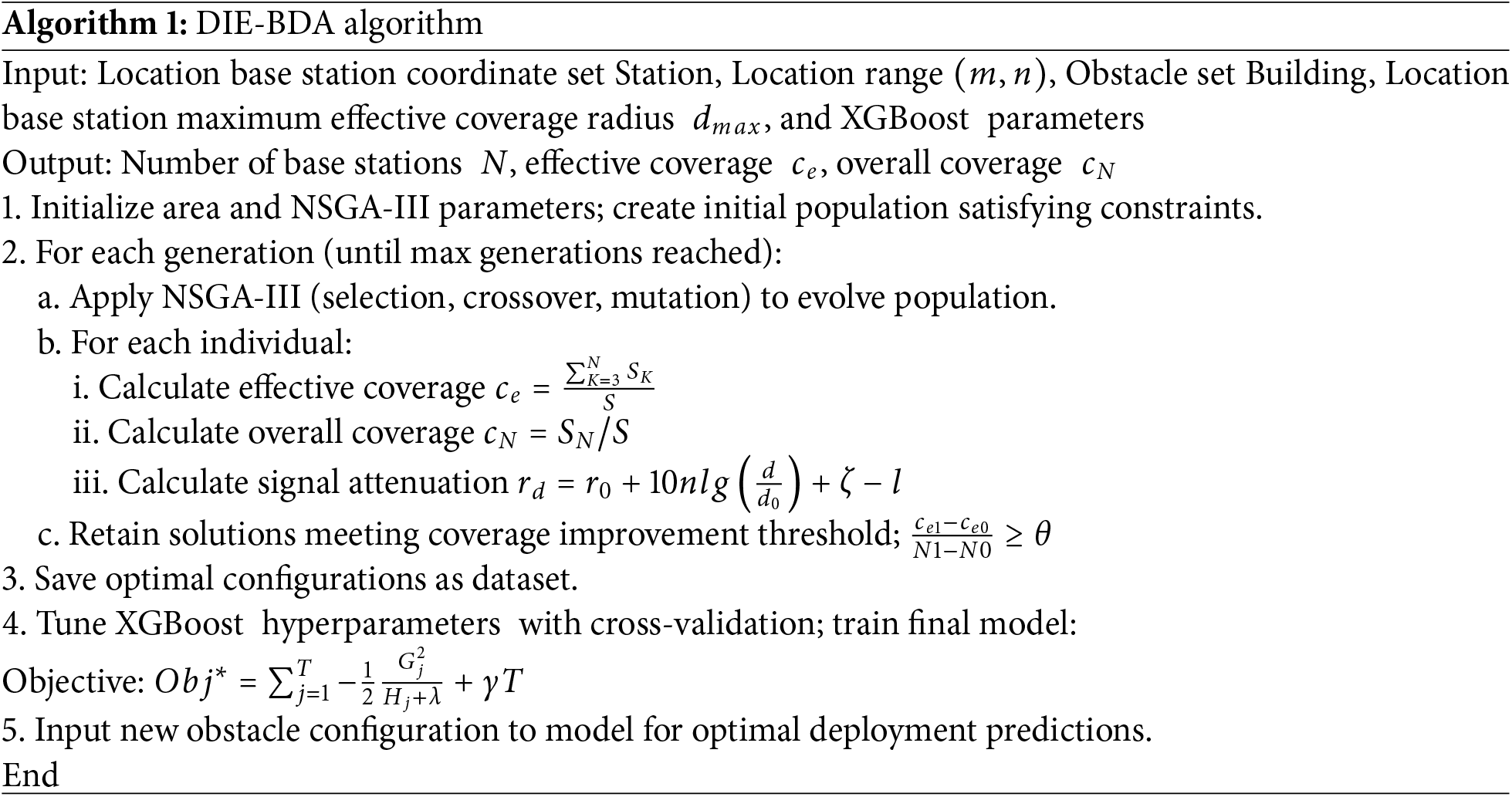
The computational complexity of the DIE-BDA algorithm primarily arises from two phases: data generation and model training. In the data generation phase, the NSGA-III algorithm’s complexity depends on the number of generations, population size, and the number of optimization objectives. The complexity increases with more generations and a larger population. During the training phase, the complexity of XGBoost mainly depends on the sample size, tree depth, and the number of cross-validation folds. Once the model is trained, the DIE-BDA algorithm allows for efficient prediction by inputting the positions of new obstacles, which requires minimal computation. This makes the approach practical for real-world applications where quick deployment decisions are needed.

3.1 Wireless Positioning Base Station Deployment Model

In our previous work [2], we introduced a Deployment and Placement Strategy for Multi-Objective Optimization methodology that accounts for signal attenuation caused by penetrable obstacles. This methodology utilizes genetic algorithms to determine the optimal deployment locations for base stations. Building on this foundation, the current study extends the applicability of the deployment strategy by addressing scenarios with dynamically changing obstacles. The deployment strategy in this study utilizes a grid-based approach, which is widely used to simplify node coverage optimization in sensor networks. By discretizing the deployment area, it becomes feasible to apply multi-objective optimization techniques to achieve a balance between coverage and energy efficiency.

The localization environment map is projected onto a two-dimensional coordinate system and rasterized into a rectangular region. The grid size is denoted by Δ, which represents the resolution or granularity of the rasterized localization area in two-dimensional space. Assume the localization area is a rectangular region with dimensions m∗n, and the grid resolution is Δ. Then, the localization area is divided into M grid cells, with each cell having an area of Δ2. The total number of grid cells M is calculated as: M=mnΔ2. For convenience, the positioning base stations are only allowed to be placed at the vertices of the grid cells in the rasterized map. Each vertex has two deployment options: deployed or undeployed. A two-dimensional decision matrix is defined to represent the deployment status at each vertex within the rasterized localization area, as shown in Eq. (1).

G=[g(x,y)][(mΔ)+1]×[(nΔ)+1](1)

Eq. (2) defines vertex (x,y) in a two-dimensional decision matrix G, where g(x,y) is either 1 or 0, indicating whether a localization base station is deployed at vertex x. The rasterized region contains a total of (mΔ)(nΔ) cells, which correspond to [(mΔ)+1][(nΔ)+1] vertices. Therefore, the matrix elements are equivalent to the number of vertices.

g(x,y)={1,Deploymentoflocalizationbasestationatpoint(x,y)0,Nolocalizationbasestationdeployedatpoint(x,y)(2)

The configuration of obstacles and base stations in this environment is illustrated in Fig. 1, where obstacles are distributed across the environment and represented on the two-dimensional grid, along with the allowable base station deployment points.

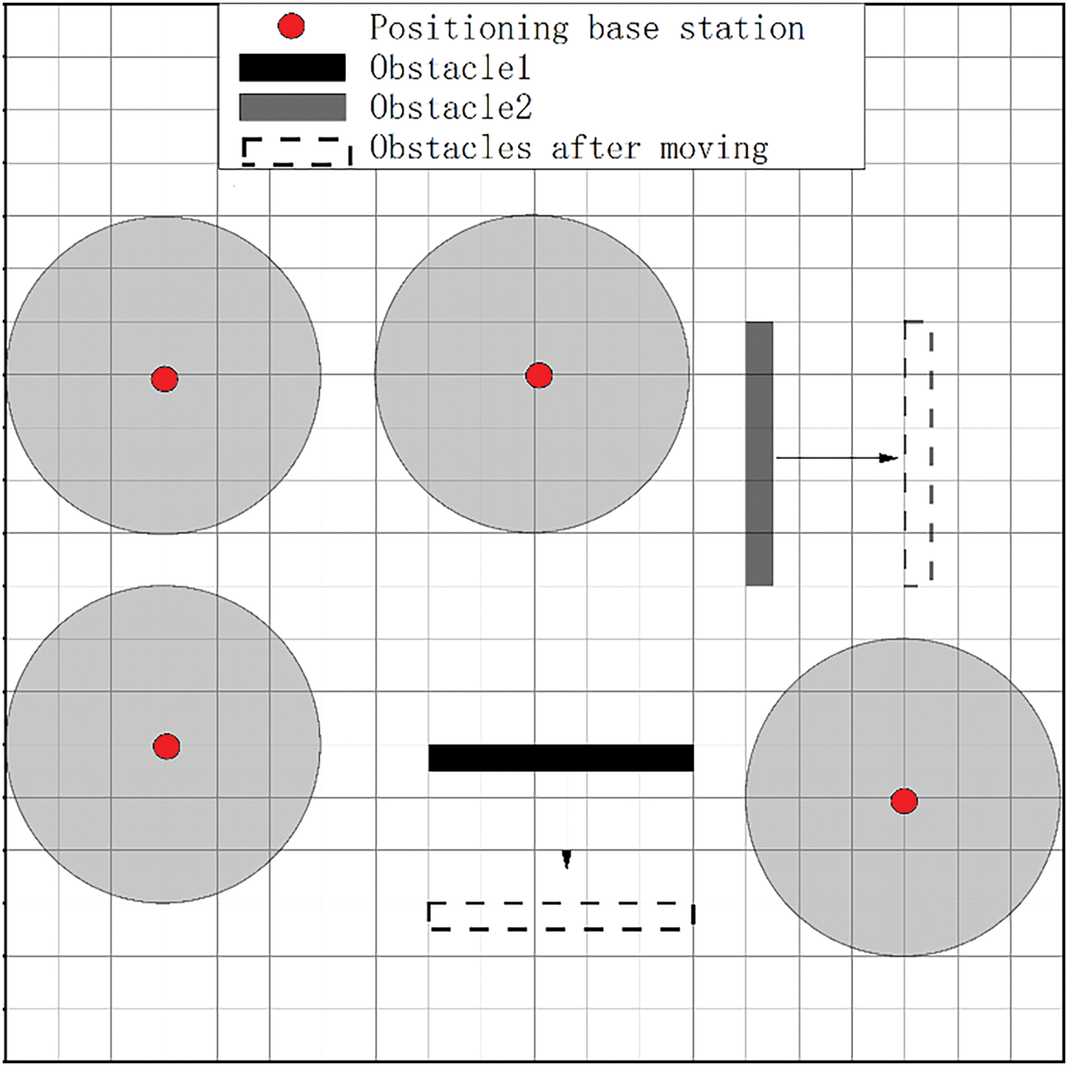
Figure 1: Map of obstacles and deployment of base stations

In Fig. 2, A, B, and C correspond to the three localization base stations, with the circles depicting their signal-sensing ranges. The overlapping gray region in the center indicates the 3-degree coverage area. The localization algorithm significantly localizes the target when the target node is within or above this area.

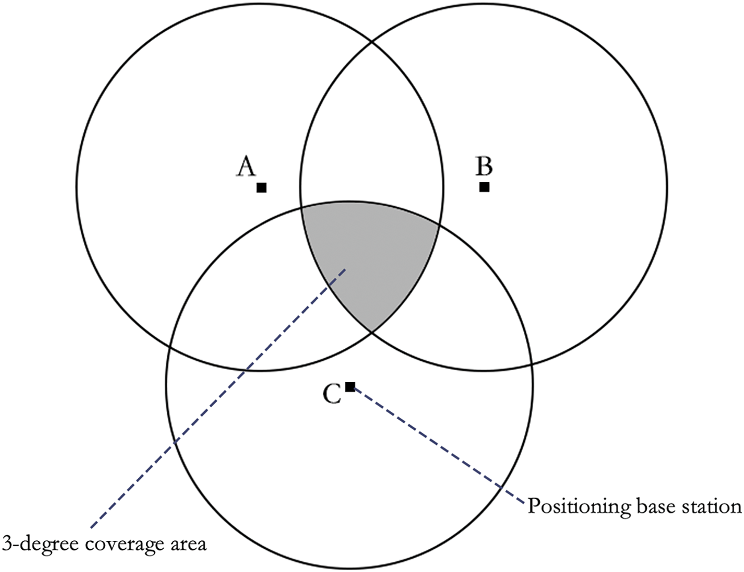
Figure 2: Signal awareness coverage

For an area to have effective coverage, it must receive signals from at least three base stations. The effective coverage ratio is defined as the ratio of the effective coverage area to the total area of the localization area. It can be represented by the equation

ce=∑K=3NSKS(3)

where ce represents the effective coverage, SK denotes the area covered by K-degree coverage (i.e., the region where each point is covered by at least K base stations), N is the total number of localized base stations, and S represents the total area of the localization region. The area SN can be considered as the area with K≥1 coverage, meaning the combined area where at least one base station provides signal coverage within the localization region. The overall coverage is then defined as the ratio of SN to the total area S of the localization region.

cN=SN/S(4)

The presence of obstacles can hinder the transmission of signals. Therefore, when there are obstacles in the indoor localization environment, it is necessary to enhance the signal attenuation model with an additional element that accounts for obstacle penetration loss, as demonstrated in Eq. (5).

rd=r0+10nlg(dd0)+ζ−l(5)

In Eq. (5), rd represents the Receive Signal Strength Indicator (RSSI) signal value at a distance d, d0 is the reference distance typically set to 1 m, and r0 is the average RSSI signal measured at d0. The signal attenuation factor n indicates the rate of signal decay with distance, commonly ranging between [2.0, 4.5], and ζ represents Gaussian noise with a mean of 0 and a standard deviation σ, while l denotes the obstacle signal penetration loss.

The obstacle signal sensing model is proposed based on the signal penetration loss. As shown in Fig. 3, A is the localization base station, the whole circle is the signal sensing region of the localization base station, and the rectangular region is the two-dimensional projection of the obstacle.

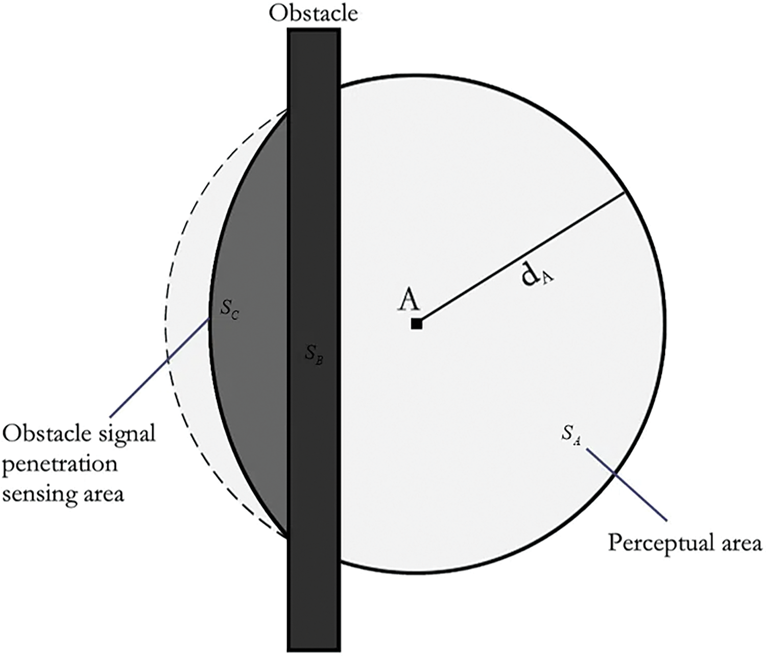
Figure 3: Obstacle signal perceived penetration loss

The signal sensing region is divided into three parts: the perceptual SA, which lies on the same side as the localization base station; the obstacle signal penetration sensing area Sc, located on the opposite side of the obstacle where signals are attenuated due to penetration; and the obstacle region SB, which represents the area occupied by the obstacle itself. Since signals within the obstacle region SB have no practical significance, they are not considered in this study, and the signal strength in this region is set to zero.

The projection of an obstacle in 2D space is defined as a rectangle O=[l,(x1O,y1O),(x2O,y2O)], l is the obstacle penetration loss, (x1O,y1O) is the obstacle start coordinates, and (x2O,y2O) is the obstacle end coordinates.

3.2 Wireless Positioning Base Station Deployment Model under the Complex Transformation of Indoor Obstacles

Multiobjective optimization often involves generating a set of Pareto-optimal solutions, from which the final solution must be selected based on application-specific criteria. Deb et al. [6] provided a foundational method for many objective optimization problems using reference-point-based approaches. In the context of conflicting objectives, this selection typically requires manual intervention, as shown by Marler et al. [22], highlighting the challenges of selecting the most suitable solution when predefined priorities are not available. Therefore, the method used to choose the optimal solution significantly impacts base station deployment. To start, we define the Effectively added base stations. Next, we address base station deployment in the presence of various obstructions. Finally, we utilize the optimized base station deployment data for different barriers to train the XGBoost model.

3.2.1 Effectively Added Base Stations

Fig. 4 illustrates the change in effective and total coverage as the number of base stations increases. As seen in the figure, both effective and total coverage improve as the number of base stations rises. Initially, there is a rapid increase in coverage, but after a certain number of base stations, the rate of improvement begins to diminish, indicating diminishing returns.

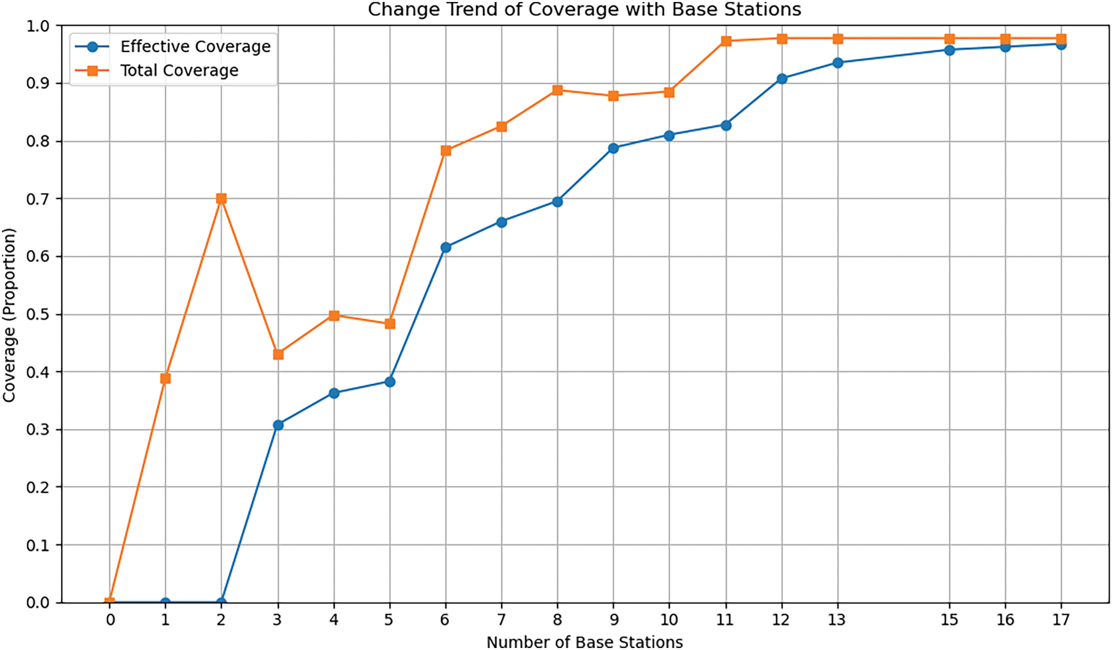
Figure 4: Change trend of coverage with base stations

To ensure efficient use of resources while maintaining high coverage, we introduce the concept of “Effectively added base stations”. A new base station is added only if the resulting increase in effective coverage exceeds a predefined threshold, denoted by θ. Specifically, in our approach, θ is set to 1%, meaning that a new base station is added only if it leads to an improvement of at least 1% in effective coverage. This ensures that each new base station significantly contributes to improving overall coverage, thereby avoiding unnecessary deployment of resources.

In security systems, high reliability and comprehensive coverage are crucial. However, over-deploying base stations can lead to wasted resources and spatial congestion. The use of θ helps balance the requirement for high coverage reliability with the need for resource efficiency, ensuring that only base stations contributing effectively to coverage are deployed. This threshold mechanism is reflected in Eq. (6).

ce1−ce0N1−N0≥θ(6)

Here, ce1 and ce0 represent the effective coverage before and after adding a base station, while N1 and N0 are the respective numbers of base stations. By adopting this approach, we optimize the network design to meet the stringent coverage requirements of security systems without unnecessary over-deployment.

3.2.2 XGBoost Modeling

The concept of boosting, particularly gradient boosting, was first introduced by Friedman [23], laying the foundation for the development of more advanced boosting techniques. XGBoost (Extreme Gradient Boosting) was later developed by Chen during his Ph.D. studies at the University of Washington, in collaboration with Guestrin [24]. XGBoost is known for its scalability and efficiency, making it a preferred choice in numerous machine learning applications.

XGBoost operates as an additive model, optimizing only the submodel in the current step during each iteration. At step m:

Fm(xi)=Fm−1(xi)+fm(xi)(7)

The objective function consists of the sum of empirical risk and structural risk (regular term):

Obj=∑i=1NL[Fm(xi),yi]+∑j=1mΩfj(8)

By substituting Eq. (7), we get

Obj=∑i=1NL[Fm−1(xi)+fm(xi),yi]+∑j=1mΩfj(9)

The notation Ω(f) represents the complexity of the sub-model f.

Taylor’s formula approximates the function f(x) with an nth-order derivative at x=x0 using an nth-order polynomial concerning Δx=x−x0. XGBoost utilizes a second-order expansion to estimate the loss function. By treating Fm−1(xi) as x0, fm(xi) as Δx, and L(yi∧,yi) as a function with respect to yi∧, The objective function is represented as

Obj=∑i=1N[gifm(xi)+12hifm2(xi)]+Ω(fm)(10)

Among these: gi=∂L∂Fm−1(xi), hi=∂2L∂2Fm−1(xi)

where L is the loss function that measures how good a prediction is. With Fm−1(x) determined, both gi and hi can be easily computed for each sample point i.

To prevent overfitting, XGBoost defines the tree-based complexity as the regular term:

Ω(f)=ΥT+12λ||ω||2(11)

In the given formula, T represents the number of leaf nodes within the trees, ω denotes the vector derived from the regression output values of all leaf nodes, and ||ω||2 indicates this vector’s squared L2 norm (also known as the Euclidean norm). The hyperparameters Υ and λ are also featured. A greater number of leaf nodes in regression trees leads to smaller regression output values.

By uniting the regularization and risk terms, we can define the sample set on node j as I(j)={xi|q(xi)=j}, where q(xi) is the index function that maps the samples to the leaf nodes. Ultimately, the following formula is derived:

Obj=∑j=1T[Gjωj+12(Hj+λ)ωj2]+ΥT(12)

In the given scenario, once the tree structure is established, the samples (xi,yi,gi,hi), and hi within each node are also determined. Specifically, Gi,Hi,T are fixed. The regression values produced by each leaf node are designed to minimize the following Equation at its quadratic function extremum: ωj∗=−GiHj+λ. They are substituting ωj∗ into Eq. (12) yields:

Obj∗=∑j=1T−12Gj2Hj+λ+γT(13)

As per the rule above, Eq. (13) indicates that a lower objective function value indicates a better tree structure for regression value output.

Upon deriving the regression value output per the rule above, researchers can infer from Eq. (13) that a smaller objective function value indicates a more optimal tree structure. According to Eq. (1), the data used to solve the base station deployment problem follows a binary categorical distribution. In the context of binary classification tasks, XGBoost is well-suited to identify patterns within the data and to construct reliable classification models. This study utilized a multi-output classifier to enable multi-label classification with XGBoost, adapting it from its original design for single-label classification. It is worth noting that the objective function in Eq. (8) serves specifically to optimize the XGBoost model during training, focusing on reducing prediction errors and enhancing generalization. This function is not directly related to handling the dynamic nature of obstacles, which is instead addressed through the diversity of training data scenarios.

4  Simulation Experiment Results Analysis

4.1 Experimental Conditions and Parameter Settings

We performed a series of simulation experiments to evaluate the effectiveness of the proposed algorithm for positioning base station deployment and carefully analyzed the results. The experiment was designed using the XGBoost and NSGA-III algorithms to determine the optimal number of base stations and the most efficient coverage rate. The experimental setup included a 12th Gen Intel(R) Core (TM) i9-12900H processor, 16.0 GB of memory, and Python version 3.9.

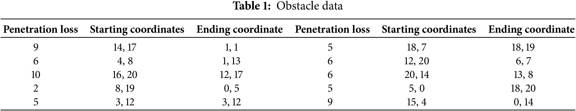
We established the deployment rules with a positioning range of 20 m × 20 m, dividing it into 400 grids. The base stations were positioned at the intersections of these grids, with a maximum signal coverage of 7 m. In the simulation, we introduced two rectangular obstacles whose positions and penetration losses varied continuously. Fig. 5 illustrates the environment in which the base stations were deployed.

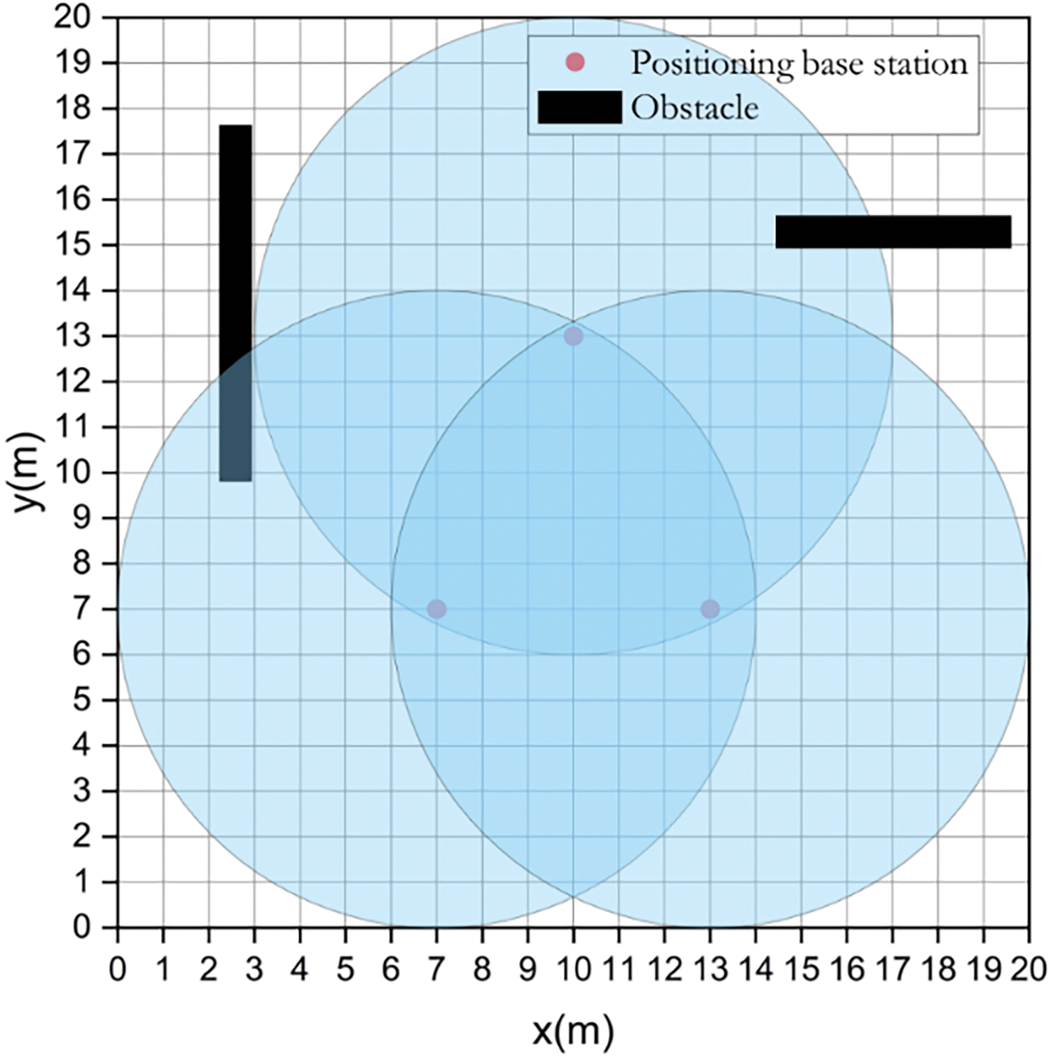
Figure 5: Base station deployment environment

Table 1 lists some of the data on the obstacles under dynamic changes.

4.1.1 NSGA-III Algorithm Parameter Settings

The multi-objective optimization problem formulated in this study includes multiple objectives, such as minimizing the number of base stations, maximizing effective coverage, and maximizing total coverage in the localization area. This optimization is subject to several constraints, including base station positioning, obstacle avoidance, and signal attenuation due to obstacles. The mathematical formulation of the optimization problem is presented below to provide a clear understanding of the objectives and the associated constraints. The multi-objective optimization problem considered in this study is solved using the NSGA-III algorithm and can be formulated mathematically as follows:

Minimizing the Number of Base Stations N, as defined in Eq. (14).

N=min[∑x=0m/Δ∑y=0n/Δg(x,y)](14)

Maximize Effective Signal Coverage ce, as defined in Eq. (15).

ce=max(∑K=3NSKS)(15)

Maximize Overall Signal Coverage cN, as defined in Eq. (16).

cN=max(SN/S)(16)

When obstacles are fixed, the NSGA-III algorithm determines the optimal solution at each iteration. We present the final results in Fig. 6.

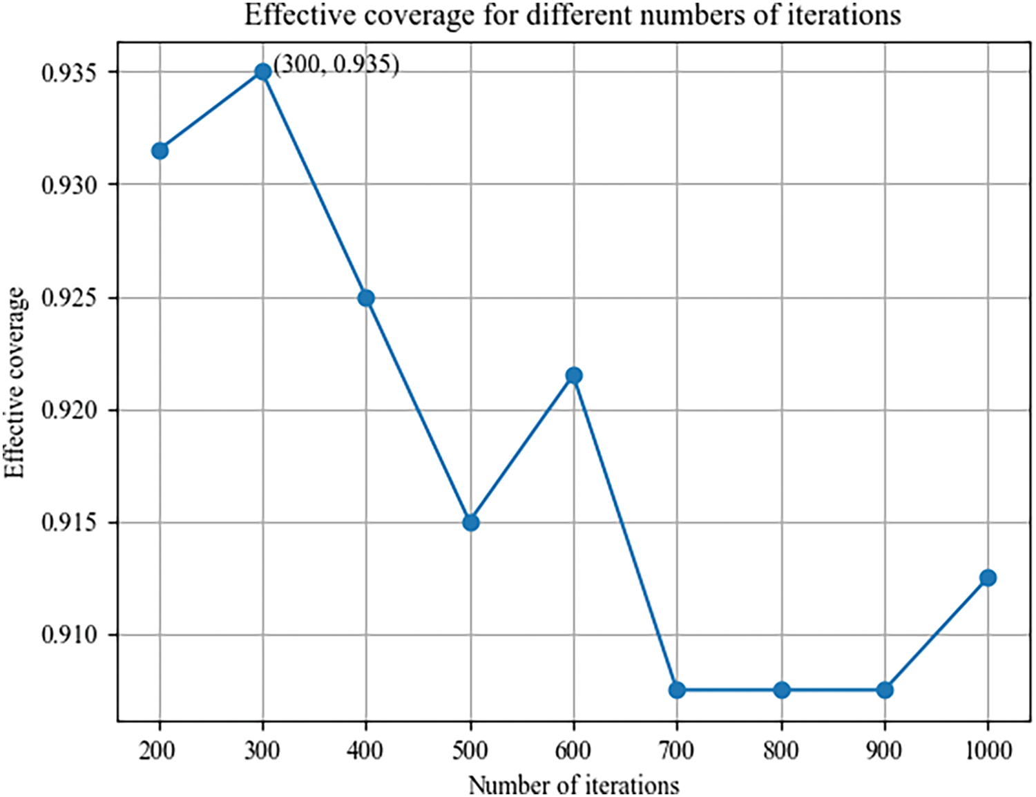
Figure 6: Effective coverage for different numbers of iterations

We observed the model results every 50 generations, from the 50th generation to the 1000th generation. The model results show that we achieve an optimal coverage rate of 0.935 after 300 generations. Therefore, the NSGA-III optimization algorithm parameter settings are as follows: 3 optimization objectives (number of base stations N, effective coverage rate ce, overall coverage rate cN; population size ning = 200; MAXGEN = 300; and the decision variable is the decision matrix G (deployment range is 20 m × 20 m, with base stations deployed at the vertices. Thus, the number of base station deployment positions is 21 × 21).

Table 2 lists some data obtained by the algorithm.

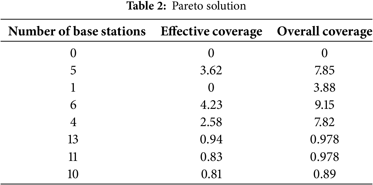
The model’s progress was tracked from iteration 50, with results recorded every 50 iterations, and the process concluded at iteration 1000. From the model results, the optimal coverage rate of 0.9375 was achieved after 300 iterations. The optimization algorithm NSGA-III was configured with the following parameters: optimization objectives included the number of base stations (N), effective coverage rate (ce), and overall coverage rate (cN); The population size was set to 200 individuals (ning = 200); decision variables consisted of the decision matrix (G); the positioning area was 20 m × 20 m with base stations deployed at vertices, resulting in a total of 21 × 21 deployment locations for base stations. Table 2 contains some of the data solved by this algorithm.

4.1.2 XGBoost Parameter Settings

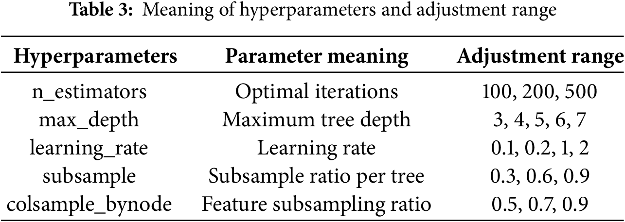
K-fold cross-validation is a widely used statistical method for hyper-parameter tuning to evaluate generalization ability [25]. In K-fold cross-validation, the training set is divided into K subsets, with K-1 subsets used as test data and the remaining subset used as validation data in each K iteration. The results of each iteration are used to calculate the accuracy rate, and the average of the K results is taken as the final accuracy rate, providing an estimate of the algorithm’s accuracy. We utilized the XGBoost algorithm to predict the unconfined compressive strength of the training set using various parameter combinations and the K-fold cross-validation method to obtain the final results. With K set to 10, we identified the best-performing parameter through cross-validation as the optimal parameter.

Table 3 displays the significance and adjustment range of the optimized parameters.

4.1.3 Model Evaluation Metrics

The XGBoost algorithm does not require predefined relationships between input and output variables, and the final performance of the model is determined by the hyperparameters [26]. Therefore, there is a need for one of the Hyperparameter tuning. Upon completing hyperparameter tuning, it was found that using the optimal hyperparameters and validating the model on the test set leads to an accuracy score that effectively represents the model’s classification accuracy. The F1 score is a comprehensive metric that considers both precision and recall. F1 scores, which range from 0 to 1, indicate better model performance with higher values. As a result, both the accuracy score and F1 score is utilized to evaluate the model’s classification accuracy. The formulas for accuracy, recall, precision, and F1 score can be found in Eqs. (17)–(20), respectively.

Accuracy=TP+TNTP+TN+FP+FN(17)

Precision=TPTP+FP(18)

Recall=TPTP+FN(19)

F1=2∗Precision∗RecallPrecision+Recall(20)

In this scenario, TP indicates a true positive, TN stands for a true negative, FP represents a false positive, and FN denotes a false negative. The dataset was randomly divided, with 80% used for training and 20% for testing, resulting in an impressive accuracy rate of 99.18% and an F1 score of 99.15%.

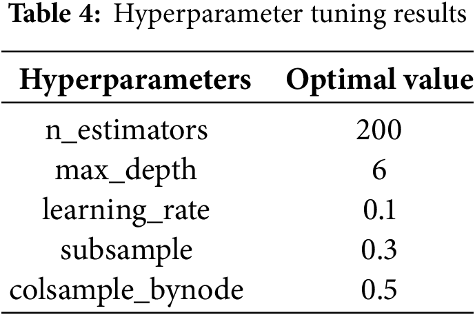
We have defined the parameters for the final XGBoost model as follows: the labels are based on obstacles, with ten corresponding obstacle labels, and decision matrix G represents the features. The hyperparameters are detailed in Table 4.

4.2 Experimental Results and Analysis

This study compares the DIE-BDA and H-BOA algorithms for WSN topology, focusing on their ability to select optimal solutions automatically. Additionally, it compares the performance of the DIE-BDA algorithm with the DPS-MOO algorithm. The Pareto solutions generated by each algorithm consist of approximately six base stations. The main objective of the analysis is to compare the computation time required for determining the optimal deployment strategy, as well as the effective coverage rate and coverage rate with six base stations for each algorithm. The experimental results are presented in Fig. 7.

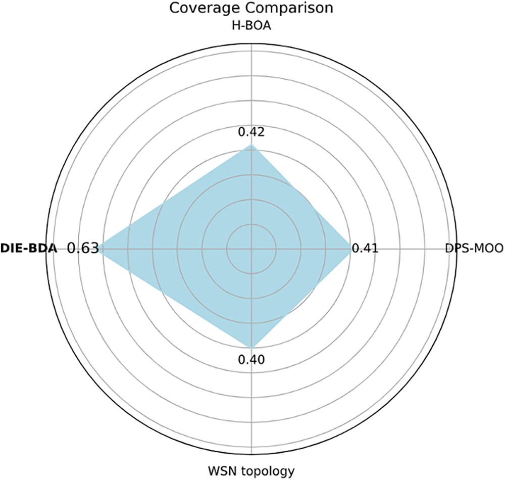
Figure 7: Coverage rate of different algorithms

The illustration displays the effective coverage rates of four algorithms across six base stations without requiring the manual selection of Pareto solutions. The H-BOA algorithm demonstrates higher deployment efficiency than the WSN topology and DPS-MOO algorithm by not considering the influence of obstacles during computation. In contrast, Li’s DPS-MOO algorithm considers signal penetration loss through obstacles, resulting in slightly higher deployment efficiency than the WSN topology model, which assumes zero signal perception when traversing obstacles.

Furthermore, the DIE-BDA algorithm effectively increased the number of base stations by eliminating ineffective solutions from the Pareto-optimal solutions. The DIE-BDA algorithm achieves an effective coverage rate of 63% at six base stations, outperforming the H-BOA algorithm, WSN topology algorithm, and DPS-MOO algorithm.

In security systems, rapidly calculating an optimal deployment strategy in response to moving obstacles is crucial for effectively stationing personnel. The algorithm developed in this study identifies the best coverage rate when deploying 13 stations, ensuring maximum utilization of each station. Illustratively, Fig. 8 demonstrates the effective coverage rates of the H-BOA algorithm, the WSN topology algorithm, and the DPS-MOO algorithm under different iterations while maintaining a fixed number of 13 stations to ensure maximum coverage. The analysis of the figure indicates that the H-BOA algorithm levels off an ineffective coverage rate after 200 iterations, which is attributed to its failure to consider obstacle impacts. Conversely, the WSN topology and DPS-MOO algorithms achieve stability after 300 iterations.

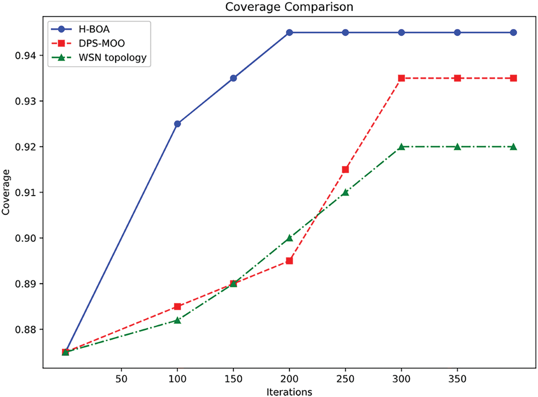
Figure 8: The iteration process of effective coverage rate

To evaluate the performance of various algorithms, including the H-BOA algorithm for 200 iterations, the WSN topology algorithm, and the DPS-MOO algorithm for 300 iterations, we calculated and compared their execution times with the DIE-BDA algorithm introduced in this paper. Given the time-sensitive nature of the data, deriving a single execution time was not feasible. Therefore, we executed each algorithm ten times and recorded the time taken for each run to assess the variation across these executions. The time consumption for each algorithm is depicted in Fig. 9. The observed fluctuations in execution times were relatively minimal, allowing us to use the average execution time as a reliable comparison metric. Notably, the DIE-BDA algorithm exhibited significantly shorter solving times compared to the other three algorithms.

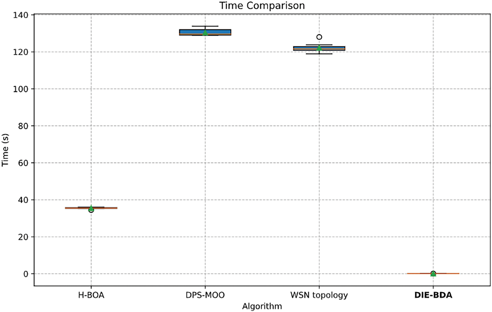
Figure 9: Time required to achieve optimal coverage rate

The final step involves selecting the average time needed for each algorithm to establish the optimal deployment strategy. This time will be the ultimate criterion for comparing the effective coverage rate and time. We will assess both metrics at maximum overall coverage by deploying 13 base stations.

Based on the decision matrix, plot the locations of the 13 base stations in the two-dimensional space depicted in Fig. 10.

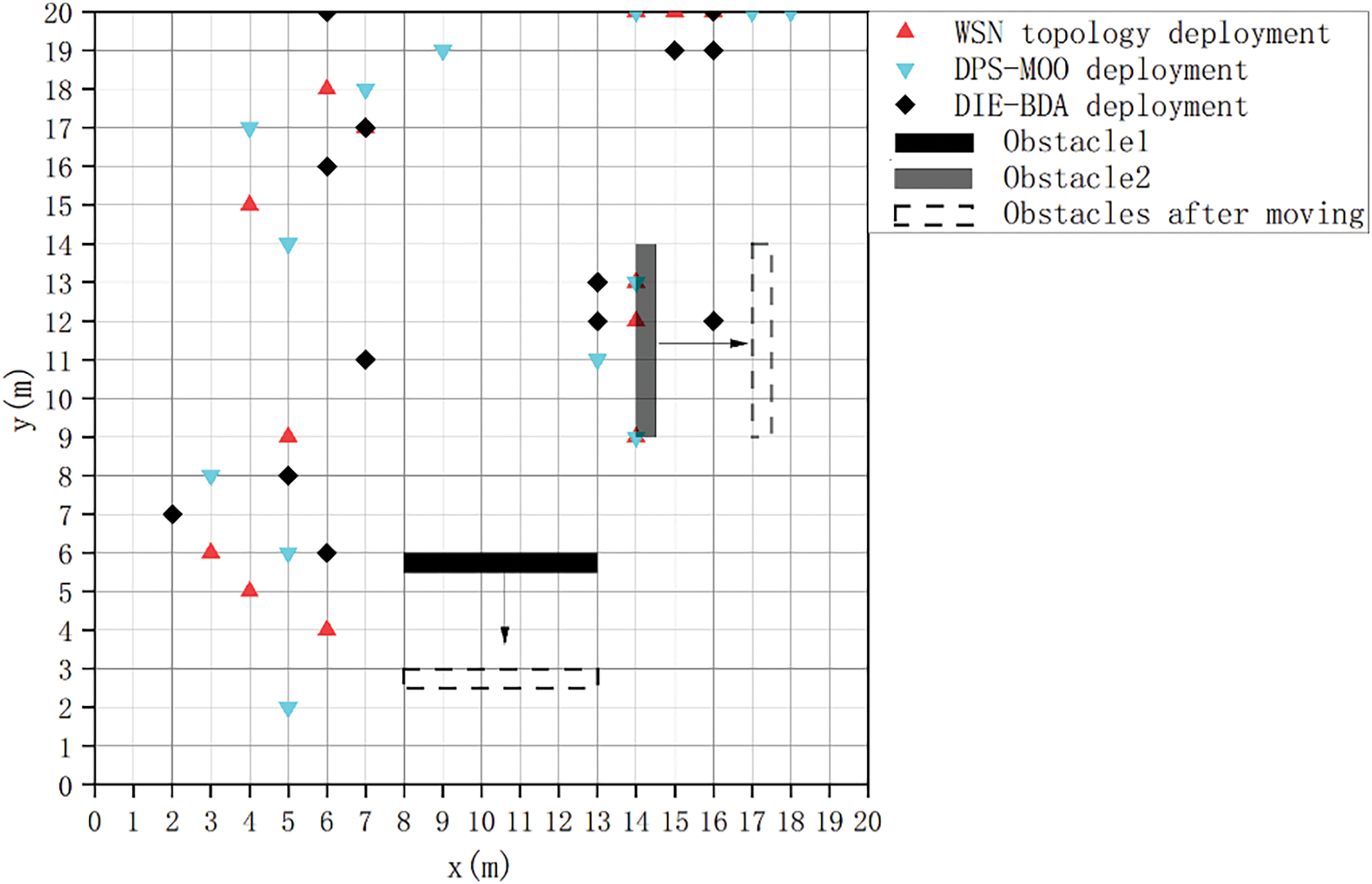
Figure 10: Comparison of different models of base station deployment

Table 5 presents the final experimental results comparing different models of base station deployment.

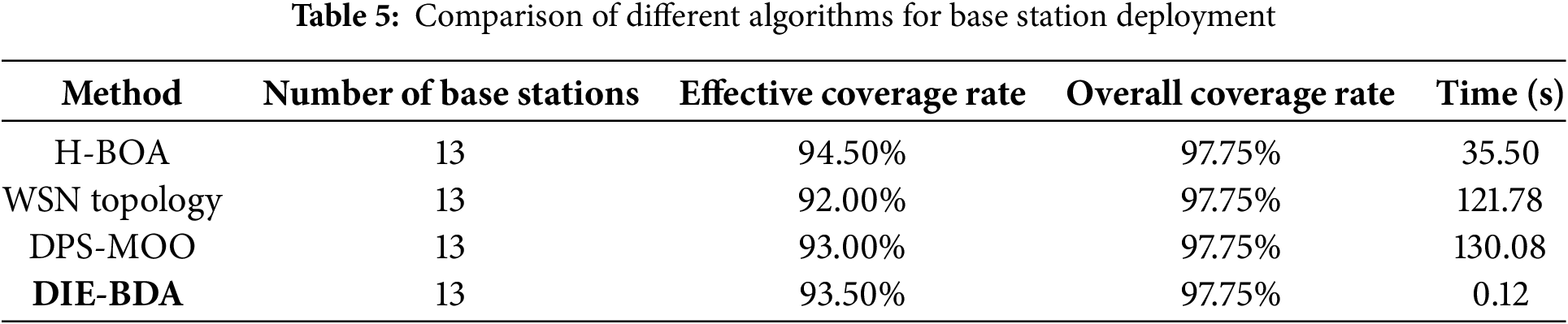
Table 5 presents the results obtained by the H-BOA algorithm, WSN topology algorithm, DPS-MOO algorithm, and DIE-BDA algorithm in this study. The H-BOA algorithm’s inability to account for the impact of obstacles results in a superior efficiency in computing deployment results compared to that of the WSN topology algorithm and DPS-MOO algorithm. The WSN topology algorithm considers signals to become zero when passing through obstacles, whereas the DPS-MOO algorithm, developed by Li, considers signal attenuation when penetrating obstacles. This results in slightly lower computing deployment efficiency than the WSN topology algorithm but higher average adequate coverage. The DIE-BDA algorithm accounts for the impact of moving obstacles. It can compute deployment strategies in approximately 0.12 s, a significantly faster processing time than the other three algorithms. The DIE-BDA algorithm achieves higher average adequate coverage in deployment results than the WSN topology algorithm and the DPS-MOO algorithm by introducing practical addition of base stations. Notwithstanding the impact of obstacles, the coverage rate approaches that of the H-BOA algorithm without obstacle considerations.

5  Conclusion

The DIE-BDA algorithm, proposed for deploying beacons in dynamic indoor environments within security systems, addresses the optimal deployment of nodes in a two-dimensional space subject to multiple dynamic obstacles. The method defines a practical approach for adding base stations and improving overall deployment efficiency. This study collected optimal deployment results under various obstacle positions in the environment and trained an XGBoost model to enhance the efficiency of recalculating optimal deployment strategies. This paper compares the DIE-BDA algorithm with the H-BOA algorithm, WSN topology algorithm, and DPS-MOO algorithm based on adequate signal coverage and time consumption for re-solving deployment strategies. The results demonstrate that in security systems where obstacle positions change dynamically, the DIE-BDA algorithm can quickly compute optimal deployment strategies, achieving effective coverage rates close to those of deployment algorithms that do not consider obstacles.

Although the DIE-BDA algorithm has demonstrated effectiveness in responding to dynamic obstacles, it has certain limitations. The algorithm relies on predefined starting and ending positions of obstacles and does not account for real-time changes in their locations. This limitation reduces its applicability in highly complex and continuously changing environments. Furthermore, the current algorithm lacks the capability to automatically recognize and track obstacles, which restricts its ability to update environmental information in real-time. Future research could address this by integrating computer vision and sensor technologies to enable automatic recognition and real-time tracking of obstacle locations, thereby enhancing the algorithm’s adaptability and efficiency in dynamic environments.

Additionally, while this study has validated the effectiveness of the DIE-BDA algorithm in recalculating optimal base station positions in response to dynamic obstacles, future research will focus on the practical challenge of physically relocating base stations. A key priority will be the integration of path planning algorithms to optimize movement paths, thereby minimizing relocation time and energy consumption. Such an enhancement would enable base stations to dynamically adjust their positions in real-time, significantly improving adaptability—particularly in security systems where frequent layout changes are common.

Acknowledgement: We would like to thank Xi’an University of Science and Technology for the support and help they have given us.

Funding Statement: This work received no specific funding for this study.

Author Contributions: The authors confirm contribution to the paper as follows: study conception and design: Aiguo Li; data collection: Aiguo Li, Yunfei Jia; analysis and interpretation of results: Aiguo Li, Yunfei Jia; draft manuscript preparation: Yunfei Jia. All authors reviewed the results and approved the final version of the manuscript.

Availability of Data and Materials: The data that support the findings of this study are available from the corresponding author on reasonable request.

Ethics Approval: Not applicable.

Conflicts of Interest: The authors declare no conflicts of interest to report regarding the present study.

References

1. Wu H, Liu Z, Hu J. Multi-objective optimization of RSSI sensor deployment considering obstacles for indoor positioning. Geomat Inf Sci Wuhan Univ. 2023;48(3):471–9. doi:10.13203/j.whugis20200421. [Google Scholar] [CrossRef]

2. Li A, Yang J. Multi-objective optimization algorithm for indoor positioning sensor deployment based on wireless network. In: Proceedings of the 2022 12th International Conference on Communication and Network Security; 2022; New York, NY, USA: Association for Computing Machinery. p. 110–6. doi:10.1145/3586102.3586138. [Google Scholar] [CrossRef]

3. Shwartz-Ziv R, Armon A. Tabular data: deep learning is not all you need. Inf Fusion. 2022;81(1):84–90. doi:10.1016/j.inffus.2021.11.011. [Google Scholar] [CrossRef]

4. Grinsztajn L, Oyallon E, Varoquaux G. Why do tree-based models still outperform deep learning on typical tabular data? Adv Neural Inf Process Syst. 2022;35:507–20. [Google Scholar]

5. Ma D, Duan Q. A hybrid-strategy-improved butterfly optimization algorithm applied to the node coverage problem of wireless sensor networks. Math Biosci Eng. 2022;19(4):3928–52. doi:10.3934/mbe.2022181. [Google Scholar] [PubMed] [CrossRef]

6. Deb K, Jain H. An evolutionary many-objective optimization algorithm using reference-point-based nondominated sorting approach, part i: solving problems with box constraints. IEEE Trans Evol Comput. 2013;18(4):577–601. doi:10.1109/TEVC.2013.2281535. [Google Scholar] [CrossRef]

7. Khalaf OI, Abdulsahib GM, Sabbar BM. Optimization of wireless sensor network coverage using the bee algorithm. J Inf Sci Eng. 2020;36(2):377–86. doi:10.6688/JISE.202003_36(2).0015. [Google Scholar] [CrossRef]

8. Aje OF, Josephat AA. The particle swarm optimization (PSO) algorithm application-a review. Global J Eng Technol Adv. 2020;3(3):001–6. doi:10.30574/gjeta.2020.3.3.0033. [Google Scholar] [CrossRef]

9. Mazloomi N, Gholipour M, Zaretalab A. Efficient configuration for multi-objective QoS optimization in wireless sensor network. Ad Hoc Netw. 2022;125(4):102730. doi:10.1109/JSEN.2022.3233361. [Google Scholar] [CrossRef]

10. Elhoseny M, Tharwat A, Yuan X, Hassanien AE. Optimizing k-coverage of mobile WSNS. Expert Syst Appl. 2018;92(3):142–53. doi:10.1016/j.eswa.2017.09.008. [Google Scholar] [CrossRef]

11. Xu Z, Guo Y, Saleh JH. Multi-objective optimization for sensor placement: an integrated combinatorial approach with reduced order model and gaussian process. Measurement. 2022;187(2):110370. doi:10.1016/j.measurement.2021.110370. [Google Scholar] [CrossRef]

12. Bouzid SE, Seresstou Y, Raoof K, Omri MN, Mbarki M, Dridi C. MOONGA: multi-objective optimization of wireless network approach based on genetic algorithm. IEEE Access. 2020;8:105793–814. doi:10.1109/ACCESS.2020.2999157. [Google Scholar] [CrossRef]

13. Yarinezhad R, Hashemi SN. A sensor deployment approach for target coverage problem in wireless sensor networks. J Ambient Intell Humaniz Comput. 2023;14(5):5941–56. doi:10.1007/s12652-020-02195-5. [Google Scholar] [CrossRef]

14. Chowdhury A, De D. Energy-efficient coverage optimization in wireless sensor networks based on voronoi-glowworm swarm optimization-k-means algorithm. Ad Hoc Netw. 2021;122(10):102660. doi:10.1016/j.adhoc.2021.102660. [Google Scholar] [CrossRef]

15. Qiu Y, Ma L, Priyadarshi R. Deep learning challenges and prospects in wireless sensor network deployment. Arch Computat Methods Eng. 2024;31:1–24. doi:10.1007/s11831-024-10079-6. [Google Scholar] [CrossRef]

16. Salama R, Al-Turjman F, Bordoloi D, Yadav SP. Wireless sensor networks and green networking for 6G communication—An overview. In: 2023 International Conference on Computational Intelligence, Communication Technology and Networking (CICTN); 2023; Ghaziabad, India: IEEE. p. 830–4. doi:10.1109/CICTN57981.2023.10141262. [Google Scholar] [CrossRef]

17. Liu Y, Li Q. Coverage algorithm based on perceived environment around nodes in mobile wireless sensor networks. Wirel Pers Commun. 2023;128(4):2725–40. doi:10.1007/s11277-022-10067-8. [Google Scholar] [CrossRef]

18. Etancelin J-M, Fabbri A, Guinand F, Rosalie M. DACYCLEM: a decentralized algorithm for maximizing coverage and lifetime in a mobile wireless sensor network. Ad Hoc Netw. 2019;87(3):174–87. doi:10.1016/j.adhoc.2018.12.008. [Google Scholar] [CrossRef]

19. Chen L, Xu Y, Xu F, Hu Q, Tang Z. Balancing the trade-off between cost and reliability for wireless sensor networks: a multi-objective optimized deployment method. Appl Intell. 2023;53(8):9148–73. doi:10.1007/s10489-022-03875-9. [Google Scholar] [CrossRef]

20. Zhu X, Zhou M. Multiobjective optimized deployment of edge-enabled wireless visual sensor networks for target coverage. IEEE Internet Things J. 2023;10(17):15325–37. doi:10.1109/JIOT.2023.3262849. [Google Scholar] [CrossRef]

21. Ishibuchi H, Imada R, Setoguchi Y, Nojima Y. Performance comparison of NSGA-II and NSGA-III on various many-objective test problems. In: 2016 IEEE Congress on Evolutionary Computation (CEC); 2016; Vancouver, BC, Canada: IEEE. p. 3045–52. doi:10.1109/CEC.2016.7744174. [Google Scholar] [CrossRef]

22. Marler R, Arora J. Survey of multi-objective optimization methods for engineering. Struct Multidiscipl Optim. 2004;26(5):369–95. doi:10.1007/s00158-003-0368-6. [Google Scholar] [CrossRef]

23. Friedman JH. Greedy function approximation: a gradient boosting machine. Ann Stat. 2001;29(5):1189–232. doi:10.1214/aos/1013203451. [Google Scholar] [CrossRef]

24. Chen T, Guestrin C. XGBoost: A scalable tree boosting system. In: Proceedings of the 22nd ACM SIGKDD International Conference on Knowledge Discovery and Data Mining; 2016; New York, NY, USA: Association for Computing Machinery. doi:10.1145/2939672.2939785. [Google Scholar] [CrossRef]

25. Kokkinos Y, Margaritis KG. Managing the computational cost of model selection and cross validation in extreme learning machines via Cholesky, SVD, QR and eigen decompositions. Neurocomputing. 2018;295(4):29–45. doi:10.1016/j.neucom.2018.01.005. [Google Scholar] [CrossRef]

26. Li Y, Shami A. On hyperparameter optimization of machine learning algorithms: theory and practice. Neurocomputing. 2020;415(1):295–316. doi:10.1016/j.neucom.2020.07.061. [Google Scholar] [CrossRef]