Efficient Cooperative Target Node Localization with Optimization Strategy Based on RSS for Wireless Sensor Networks

1  Introduction

Wireless sensor networks (WSN) can be randomly deployed on a large scale in monitoring areas to achieve the perception, collection, and processing of regional environment or event information, especially in areas where people cannot reach dangerous areas, leveraging their advantages of 24-h uninterrupted monitoring [1]. One of the main contents of environmental or event information monitoring is to grasp the required data or the location of anomalies to provide services for correct decisions. Therefore, obtaining location data is one of the important technologies for WSN applications [2,3]. The design of node localization algorithms is constrained by the inherent characteristics of WSN, such as the dense deployment of nodes, limited communication and computing capabilities, and low-cost design for long-term network operation [4,5]. In practical applications, it is also necessary to consider the interference caused by obstacles, fading, and noise in communication channels. Therefore, the design of positioning algorithms should consider multiple factors to achieve an appropriate balance between performance and cost [6].

Positioning algorithms are usually divided into non-ranging algorithms and ranging algorithms [7–9]. TOA (Time of Arrival), TDOA (Time Difference of Arrival), AOA (Angle-of-Arrival), and RSSI (Received Signal Strength Indication) belong to the category of the ranging algorithms, which obtain the node position coordinates by measuring the distance between nodes or wireless signal arrival angle information, combined with positioning algorithms. The non-ranging algorithm can locate without inter-node distance or orientation information, but the positioning accuracy is generally low due to the complex network topology structure and the lack of full use of known information. In ranging algorithms, TOA/TDOA and AOA ranging techniques are limited by the power consumption of WSN nodes, and the algorithm design cannot achieve satisfactory positioning results. The RSSI ranging method utilizes the node’s built-in RF transmission function, and based on the RSS, models the wireless signal propagation to obtain range information [10]. The advantages of using this method are low power consumption and cost, but the disadvantages are also obvious, that is, RF signal transmission is greatly affected by environmental factors such as occlusion and multipath effects, and channel fading is fast. Even at the same distance and in the same environment, RSSI values may fluctuate [11]. In RF signal transmission modeling, the wireless path fading factor reflects the overall environmental impact [12]. Therefore, the determination of the fading factor not only affects the ranging accuracy but also is crucial for the accurate measurement of RSSI values. The general method is to take multiple measurements and refining algorithms to reduce ranging errors [13].

Given that wireless signal transmission modeling is the foundation of RSS ranging, some scholars have attempted to estimate its parameters. In [14], based on a detailed study of the statistical characteristics of RSS measurements, the authors put forward a new weighted algorithm based on RSSI physical distance to improve the positioning accuracy of traditional positioning algorithms, which achieved significant advantages in positioning precision. In [15], to raise the precision of RSS ranging, the authors put forward an RSSI-based distribution positioning method (RDL), which can achieve high positioning accuracy without dense deployment of nodes. They also analyzed the distribution properties of different nodes at fine-grained distances and constructed a cell-positioning model. The results showed that compared with existing methods, the positioning accuracy of RDL has been improved by 50%, with an error of less than 1.5 m. In [16], the authors first explained the factors that affect positioning precision, including the number and position of sensors, the quality of received signals, and the principle of using the AOA, TDOA, and RSSI to achieve positioning, and then the authors used the reference nodes and the arrival interval for node positioning. The simulation showed that considering time synchronization, the system achieves lower average error for estimating when using RSSI positioning, indicating that RSSI-based measurements provide higher accuracy and precision during positioning.

Also based on improving the precision of RSS positioning, both Bayesian and non-Bayesian estimation methods are applied. The shortcoming of the Bayesian estimation method is that the communication cost and computing burden are large. Particle filter technology is an implementation method of Bayesian estimation, especially when dealing with nonlinear and non-Gaussian systems, approximating the posterior probability distribution in Bayesian estimation through the Monte Carlo method. However, particle filter technology often encounters difficult problems such as particle degeneration and impoverishment [17], leading to a decline in the positioning performance of WSN nodes or even making it impossible to implement positioning. The non-Bayesian estimation method treats the location coordinates of the node to be located as the determined undiscovered parameters and then uses methods such as the least squares (LS) estimation method [18] or the maximum likelihood (ML) estimation method [19] to obtain the positioning solution. In [20], the authors studied the LS collaborative localization problem under an arbitrary non-line of sight (NLOS) ranging bias, and proposed the positioning error boundary of a network. In this paper, starting from the Cramer Rao lower limit (CRLB), by quantifying LS, distance square LS, and weighted LS (WLS) positioning accuracy deviation, the authors put forward a simple LS distributed algorithm that integrates squared distance relaxation and Gaussian variation information for collaborative localization. In [21], the authors proposed a new hybrid collaborative localization scheme based on distance and angle measurements, which modifies the TOA-AOA and AOA-RSS-based linear least squares (LLS) hybrid schemes and proposed an optimized version of LLS estimation. Simulation results showed that this algorithm outperforms non-collaborative algorithms and iterative nonlinear-LS algorithms based on mixture signals.

In recent years, some methods such as semi-definite programming, fingerprint matching, genetic algorithm, and RSSI quantization have also achieved good results for localization problems. In [22], a new location algorithm based on collaborative RSS was proposed by combining the semi-definite programming method to achieve real-time localization. In this algorithm, the relative error estimation and semi-definite programming (SDP) are used and the CRLB is derived for the collaborative localization based on RSS. Firstly, the logarithmic normal shadow RSS measurement model is transformed into an equivalent multiplication model. Then, the relative error analysis criterion is used together with the model to develop a non-convex estimator to approximately gain the maximum likelihood solution. Finally, semi-definite relaxation is applied to the non-convex estimation to obtain the SDP estimation. Compared with existing localization methods, the proposed SDP estimator provides significant improvements. Based on the RSSI difference and distance ratio, a new 3D positioning method is proposed in reference [23], which utilizes virtual fingerprints and bidirectional ranging to overcome the four obvious shortcomings of traditional RSSI fingerprint recognition methods. In [24], based on RSSI quantization and genetic algorithm, a two-stage centroid-positioning algorithm was proposed, which is particularly suitable for irregular target regions. Finally, an experimental environment is constructed to prove the property of the algorithm. In addition, the application of RSS-based adaptive methods and filtering techniques in obtaining target positions further improves positioning performance. According to reference [10], an adaptive ranging algorithm based on RSSI is proposed to promote the quality of ranging under constantly varying outside surroundings. This algorithm contains the RSSI estimation of the link, temperature compensation, path loss index (PLI) estimation, and inter-node interval estimation, and finally evaluates the performance of the proposed algorithm. The research on estimation algorithms of model parameters based on wireless signal transmission modeling or positioning algorithms based on RSSI ranging has made efforts to improve positioning accuracy in various aspects mentioned above. However, most of these algorithms have high computational and communication costs and require high network topology. In practical WSN positioning applications, they are often difficult to implement due to cost and power constraints.

This article focuses on the two key stages of ranging and positioning estimation. Based on intensive research of the RSSI ranging principle and the demand of positioning systems, the power-fading factor is periodically and dynamically obtained to acquire distance information. RSSI ranging calibration is performed using the regional relative distance error coefficient. By selecting the reference nodes involved in positioning, the computational complexity is reduced and the positioning efficiency is improved. Take coordinate error correction measures for the estimated position coordinates, fully utilize known information, suppress cumulative errors, and finally use the Taylor series least squares iterative refinement technique to further promote location precision. To full use the superiority of collaborative positioning, the positioning nodes that accord with the demands are upgraded to reference nodes to partake in the succedent positioning process, which effectively improves the positioning accuracy and robustness. Due to the avoidance of complex calculations caused by minimizing mathematical analysis and increasing communication volume through collaboration between all nodes in this article, effective correction measures are taken at each stage of positioning implementation to improve positioning accuracy. Therefore, compared to pure analytical algorithms and inter-node collaboration schemes, the data volume is greatly reduced in terms of communication and computational costs.

2  Principle of Distance Estimation

2.1 Ranging Model and Ranging Algorithm

By utilizing the wireless communication function of nodes in WSN and the communication control chip provided by nodes to provide RSSI measurement, RSSI value measurement can be completed without the need for additional equipment during the positioning process. It can be seen that RSSI ranging technology has low cost and power consumption, is easy to apply, and therefore has received widespread attention. When applying RSSI ranging in practical applications, the effects of multipath, diffraction, and obstacle occlusion are considered, and wireless signal transmission is modeled as

PR(d)=P+G−PL(d)=PR(d0)−10nlg(dd0)+Xσ(1)

Among them, P is the propagating power, G is the antenna gain, and PL(d) is the power consumption of the wireless signal after transmission distance d. The power consumption factor n usually ranges from 2 to 4. For reference distance d0, it is generally taken as 1 m. The PR(d0) is the received signal strength at a distance of d0 from the emission point, and Xσ is a Gaussian random quantity with zero mean. The larger the value of PR(d) measured by the receiving point, the closer the node space is.

Using the positional coordinates of known reference nodes, the signal intensity between adjacent reference nodes is obtained by periodic dynamic measurement. The real-time power consumption factor of the current reference node’s area can be obtained through the wireless signal transmission model. Considering the value of PR(d) received by reference node R0 from two other reference nodes R1 and R2 within its communication range in a wireless network, we can obtain

PR(d1)=PR(d0)−10n0lg⁡(d1d0)+Xσ(2)

PR(d2)=PR(d0)−10n0lg⁡(d2d0)+Xσ(3)

n0=PR(d2)−PR(d1)10lg⁡(d1d0)−10lg⁡(d2d0)(4)

The n0 is the dynamic power consumption factor, which reflects the influence of the current wireless channel environment on the signal energy consumption.

According to Eq. (4), the factor n0 is determined only by PR(d1) and PR(d2), as well as d1 and d2, and is independent of the measured value of PR(d0). This method dynamically obtains the RSSI measurement value at the reference node and calculates the more accurate power consumption factor in the area of the current reference node in real-time. Therefore, the calculated RSSI distance measurement is less affected by the signal transmission modeling, and the ranging accuracy is improved, thus adapting the RSSI ranging algorithm to the wireless channel. In actual ranging, the distance can be calculated by applying Eq. (1) using the obtained dynamic power consumption factor.

2.2 Obtaining the Final Ranging Value by Error Correction

Collaboration technology typically refers to the process in which nodes in a network that are capable of communication transmit messages or exchange information with each other, decentralize operations such as computation, communication, and storage, and collaborate in processing and completing tasks such as event detection [25]. Collaborative positioning means that collaborative technology is used in WSN positioning. The information sources for estimation data in WSN collaborative positioning are diverse, such as the data from sensor nodes themselves, communication data from adjacent nodes, position data of anchor nodes, and environmental characteristic data, which together form the basis and basis for collaborative positioning algorithms. By comprehensively utilizing these information sources, precise estimation and positioning of node positions can be achieved.

Decentralized optimization and cooperative positioning normally contain two-procedure: node self-positioning and data aggregation cooperation. The procedure of data aggregation cooperation is based upon the fact that the observational message between nodes has been carried out for each node in the current network (including between the unpositioned nodes and the reference nodes, between the reference nodes, and between the unpositioned nodes). In addition, the positioned unknown nodes take over the positioning message and observation message of adjacent nodes (including reference nodes and other located unknown nodes), and then some cooperative positioning method is realized to obtain more precise positioning message of unknown nodes. The diagram of the decentralized optimization and cooperative positioning procedure is shown in Fig. 1.

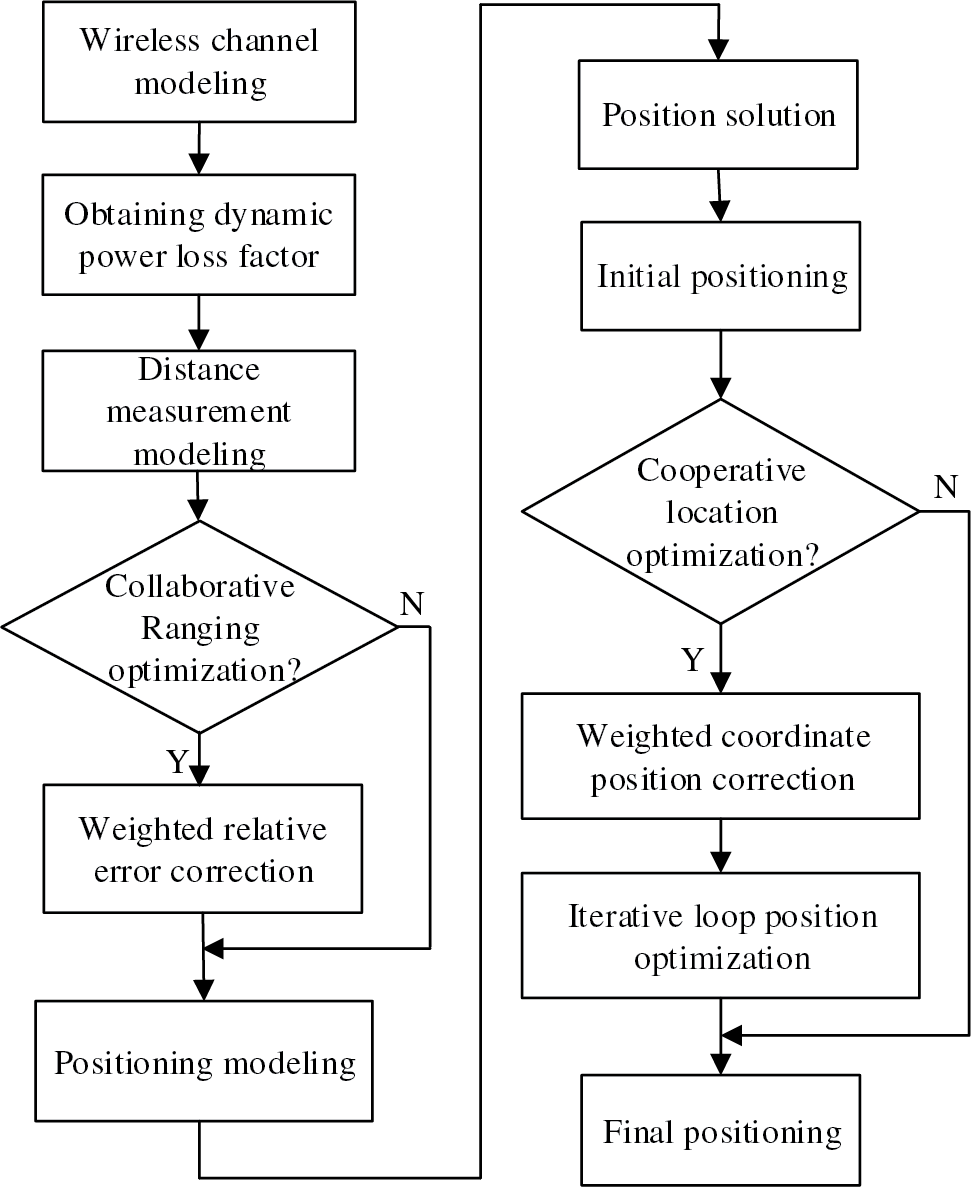
Figure 1: The diagram of the decentralized optimization and cooperative positioning process

The accuracy of distance data used for positioning estimation directly affects the positioning accuracy. Therefore, before positioning calculation, it is generally necessary to preprocess the obtained distance data to obtain the distance data with the highest accuracy possible, providing a good data foundation for subsequent positioning calculations. The preprocessing of distance data involves using suitable refinement algorithms, cyclic refinement algorithms, or iterative refinement algorithms to reduce ranging errors and obtain more accurate distance data.

Firstly, the received signal strength is measured, and then the distance between any reference node in the network and its neighboring reference nodes is modeled through wireless transmission. Then, the differential value between this distance and the physical distance calculated by the reference node is taken as the relative measurement error of RSSI at that reference node. So when ranging unknown nodes, considering the RSSI measurement error at each reference node can minimize the error caused by harsh wireless communication environments on ranging.

The reference node to be corrected in the 2-D network is denoted as S0(x0,y0), and its neighboring reference nodes are denoted as Si(xi,yi), i=1,2,⋯,n, where n is the number of neighboring reference nodes. The actual calculated distance from S0(x0,y0) to Si(xi,yi) is denoted as ri, and the distance measured through RSSI is denoted as di, i=1,2,⋯,n. The relative ranging error at reference node R0 is

μi=di−riri(5)

The weighted RSSI ranging relative error correction coefficient at the reference node S0 is

μw=∑i=1nri−didi2∑i=1n1di(6)

μw comprehensively reflects the RSSI relative measurement error of reference node S0. Here, different distance weights reflected by different RSSI values are considered to obtain the contribution of the error correction coefficient. The distance corrected by the reference node weighted RSSI ranging relative error correction coefficient is denoted as

dic=di(1+μw)(7)

where di is the measured range between the unknown location node and the reference node Si, and dic is the correction range between the unknown location node of the sensor and the reference node Si.

3  Distributed Collaborative Localization Algorithm

3.1 Node Coordinate Estimation

For the RSSI method, we choose the N reference nodes information that we received first. That is, all the received PR(d) values are queued in descending order PR(d1),PR(d2),⋯,PR(dn), and the number of PR(d) values that we have received is n in total. Define an anchor selection parameter SA as

SA=∑i=1NPR(di)∑i=1nPR(di)(8)

Set the threshold of SA to τ, only when SA≥τ, it is guaranteed that there are sufficient reference nodes to partake in the positioning estimation within a certain positioning error range. Too large or too small the value of τ will lead to a decline in positioning accuracy. We take the N reference nodes corresponding to the first PR(d) values to participate in the localization calculation. Since N is greater than or equal to 3, through experiments, in general, SA≥0.9 is sufficient.

Assuming that there are N reference nodes in the network, denoted as Si(xi,yi), i=1,2,⋯,N. Their measurement distance to the unknown node denoted as U(x,y) is di, i=1,2,⋯,N. Then the measurement modeling is as follows:

d^i=di+vi,i=1,2,⋯,N(9)

where

di=(xi−x)2+(yi−y)2(10)

vi is the measurement error.

Inserting Eq. (10) into the Eq. (9) and squaring both sides of Eq. (9), we get:

x2+y2−2xix−2yiy=(d^l−vi)2−(xi2+yi2)

Arranging the above equation, it can be expressed in matrix form as

h=Gθ+v(11)

where

G=[−2x1−2y11⋮⋮⋮−2xN−2yN1](12)

h=[d^12−(x12+y12),…,d^N2−(xN2+yN2)]T(13)

v=[2d^1v1−v12,…,2d^NvN−vN2]T(14)

θ=[xyR]T(15)

R=x2+y2(16)

Then the solution of the WLS (Weighted Least Squares) algorithm of Eq. (11) is

θ^=(GTWG)−1GTWh(17)

where

W=cov−1(v)(18)

W is a weighted matrix, and when the specific error statistical characteristics are unknown, W can be set as the unit matrix.

3.2 Node Coordinate Correction

Although the correction factor μw of range measurement can raise the range measurement precision of RSSI, it cannot reduce the random deviation in the communication environment and the positioning algorithm itself. To full use the known coordinate information of the reference nodes, we consider further correcting the estimated coordinates to improve the positioning accuracy. Use the maximum likelihood estimation method to calculate the estimated coordinates of the reference node, and then take the difference between the real coordinates of the reference node and the estimated coordinates, which is the coordinate error correction coefficient. Therefore, when estimating the positioning coordinates of unknown nodes, considering the coordinate error at the reference node used can suppress various interferences such as wireless channel environment and positioning algorithms, effectively improving positioning accuracy.

The reference node in the network is denoted as R0(x0,y0), and the neighboring reference nodes within its communication range are denoted as Ri(xi,yi),(i=1,2,⋯,n). Therefore, The position estimation coordinate of R0 obtained by applying the positioning algorithm is Rc0(xc0,yc0), and the difference between the two is used to obtain the coordinate error at reference node R0

{ex0=x0−xc0ey0=y0−yc0(19)

The position error of the ith reference node in the network is denoted as

{exi=xi−xcieyi=yi−yci(20)

Then, the weighted position error ew of the positioning region is denoted as

ewx=∑i=1Nexidic∑i=1N1dic(21)

ewy=∑i=1Neyidic∑i=1N1dic(22)

{x=xc+ewxy=yc+ewy(23)

Among them, xc and yc are the coordinate values calculated using the maximum likelihood estimation method for unknown nodes.

3.3 Location Optimization

Iterative loop refinement is an effective method to promote positioning precision. To depress the error further in coordinate estimation, the determined coordinate values are taken as initiative values and the Taylor series least squares method is used for position optimization.

According to the distance Eq. (10), so that

f(x,y)=(x−xi)2+(y−yi)2(24)

Set the initial coordinates are (x0,y0), expand Eq. (24) at (x0,y0) in a Taylor series, and ignore second-order and higher-order components

f(x,y)=f(x0,y0)+fx(x0,y0)Δx+fy(x0,y0)Δy(25)

Eq. (25) can also be written as

d^l=d^l0+axΔx+ayΔy(26)

where

d^l=(x−xi)2+(y−yi)2

d^l0=(x0−xi)2+(y0−yi)2

ax=fx(x0,y0)

ay=fy(x0,y0)

Considering errors, the above equation can be abbreviated as

h=GΔ+ε(d2)(27)

where

Δ=[ΔxΔy]T

h=[d^l−d^l0,…,d^N−d^N0]T

G=[x0−x1d^10y0−y1d^10⋮⋮x0−xNd^N0y0−yNd^N0]

Using the WLS algorithm, we can obtain an estimate of Δ as follows:

Δ=(GTWG)−1GTWh(28)

where W is the correlation matrix of measuring deviation. Moreover, the updated parameter vector can be obtained:

θ(k+1)=θ(k)+Δ(29)

3.4 Algorithm Implementation Steps

In summary, considering RSSI localization, the following algorithm (Algorithm 1) is listed:

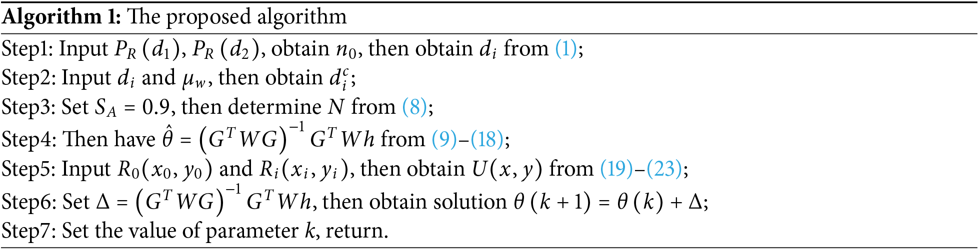
In the above algorithm process, step 1 is to perform basic RSSI ranging according to the ranging model. Step 2 is the estimated ranging stage, perform ranging correction according to Eqs. (5)–(7). Step 6 is the position optimization stage, perform iterative optimization according to Eqs. (24)–(29).

3.5 Collaborative Positioning Implementation

We introduce the conception of collaborative positioning and full use the various measurement data between nodes in the network to realize data aggregation. We carry out collaborative signal and information processing between nodes, so that a single node can consume as little energy as possible and acquire as much metrical information as possible, so as to increase the localization precision and robustness. If the located node meets certain conditions, it will be upgraded as a reference node and participate in the subsequent positioning calculation. At this time, the positioning requirements of the reference node should be considered, that is, the relatively stable RSSI-ranging environment positioning ability comparable to the reference node. According to Eqs. (2)–(4), the path loss coefficient between the reference nodes in the communication range of the upgraded node is calculated, and the mean of these loss coefficients should amount to the mean of the path loss coefficient between the other reference node in the communication range of the reference node closest to the upgraded node. Namely

|1K∑k=1KnUk−1L∑l=1LnAl|<nΔ(30)

where nUk is the path loss coefficient between K reference nodes within the transmission radius of upgraded node U, and nAl is the path loss coefficient between node U and other reference nodes within the transmission radius of the closest reference node to upgraded node L. nΔ is the threshold of the path loss coefficient for node upgradation.

4  Numerical Simulation and Performance Analysis

4.1 Simulation Scenario and Algorithm Evaluation Method

To verify the effectiveness of the algorithm proposed in this article, an RSSI ranging and positioning simulation platform was established based on Matlab software, and the localization error of the algorithm was analyzed by the experimental data. The parameters are set as follows: the positioning experiment environment is a 2-D square area of 200 m × 200 m, with 200 nodes and 20 reference nodes in a network, and the communication range of all nodes is 30~70 m adjustable. To validate effectively the algorithm performance, the same experiment was repeated after each reset of the network topology, and the average of 100 simulation experiments was used as the result.

To study the interrelation between the transmission radius of nodes, the number and the density of nodes, and the precision of the positioning algorithm, the average localization error of the nodes is used to synthetically assess the performance of the algorithm. The average localization error of the nodes is denoted as Ea

Ea=∑i=1N||pi−zi||2N⋅R(31)

Among them, N is the number of nodes to be located in a network, and the transmission radius is R. pi=[pxipyi]T is the final estimated coordinates of node i, and zi=[zxizyi]T is the true position of node i. The smaller the Ea, the more precise the positioning.

In the following simulation analysis, to evaluate the performance of the proposed algorithm, the proposed algorithm is compared with two other algorithms. The Taylor Series Expansion algorithm based on real coordinates is simply called the TSE algorithm. Since the TSE algorithm is calculated based on the real position, its positioning precision should be the highest. LS (Least Square) algorithm is the most widely used estimation method, and in a white noise environment, the LS algorithm can get gradual unbiased estimation, whereas it is biased in a colored noise environment.

4.2 Interrelation between the Positioning Precision and the Number of Reference Nodes

Positioning precision can be represented by the average localization error. At this point, the simulation experiment environment is set as follows: 100 sensor nodes are randomly distributed within the square area of 100 m×100 m, and the communication radius of the nodes is set to 40 m. The influence of the number of reference nodes on the average positioning error obtained from the experimental results is shown in Fig. 2.

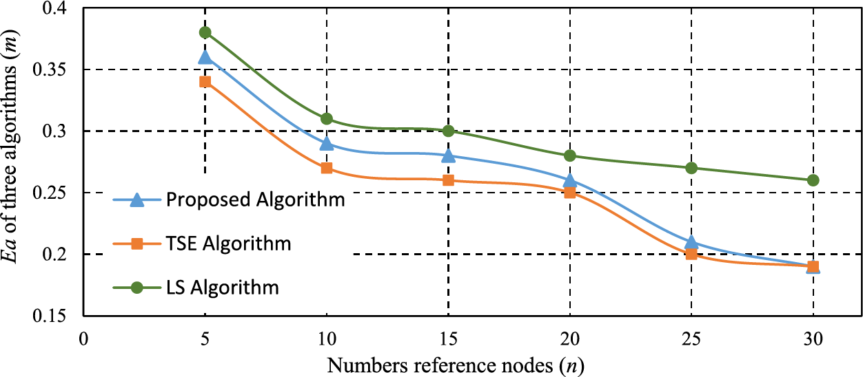
Figure 2: Effect of the number of reference nodes on the localization error

From the curve trend in Fig. 2, it can be seen that as the number of reference nodes increases, the average positioning error of the three algorithms decreases, but the performance of the proposed algorithm is much better than that of LS algorithm. When the reference node numbers exceed 20, the improvement of the LS algorithm’s positioning precision is limited and gradually tends to stabilize, while the positioning precision of the proposed algorithm is still increasing. When the reference node numbers reach 30, the average positioning error of the nodes is the same as that of the TSE algorithm, both of which are 0.19. As the proposed algorithm adopts the error correction algorithm, it can further reduce the cumulative error during the positioning process and achieve good positioning accuracy. Therefore, the positioning effect of the algorithm proposed in this article is obvious.

4.3 Interrelation between the Positioning Precision and Transmission Radius

Secondly, we study the interrelation between transmission radius and average positioning error. Here the experimental surroundings is set as follows: 200 sensor nodes in the network are randomly distributed in the 200 m × 200 m area, and the number of reference nodes is 20. The impact of transmission radius on the average positioning error of nodes is shown in Fig. 3.

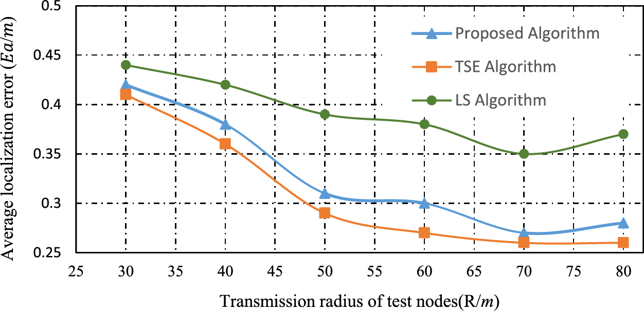
Figure 3: The effect of the transmission radius on the average localization error

From the tendency of the curve in Fig. 3, it can be seen that as the transmission radius increases, the average positioning error of the three algorithms gradually decreases. The proposed algorithm has better performance than the LS algorithm and is close to the TSE algorithm. It is thus clear that when the transmission radius is the same, the optimal reference point adopted by the proposed algorithm and the cyclic actuarial method can further reduce the positioning error. It can also be observed from the figure that when the transmission radius is 70 m, the average positioning error of the proposed algorithm no longer decreases, and even shows an increasing trend. The reason for obtaining this result is that the transmission radius has reached the maximum range of possible perception areas, the number of reference nodes no longer increases, and the positioning accuracy no longer improves. In addition, due to the accumulation of estimation errors, the positioning accuracy has decreased. On the other hand, the proposed algorithm’s performance is not sensitive to the size of the transmission radius, meaning that it can achieve high positioning accuracy without requiring a large communication power. This indicates that under the same network conditions and accuracy requirements, its positioning power consumption is lower.

4.4 Interrelation between the Positioning Precision and the Size of the Perceptual Region

Next, we will investigate the interrelation between the size of the perception area and the average positioning error. The network experimental parameters are set as follows: the reference node is 20, the transmission radius of the node is 40 m, the perception area increases, and the number of nodes also increases from 100 to 600. The impact of the perceived area size on the average positioning error is shown in Fig. 4.

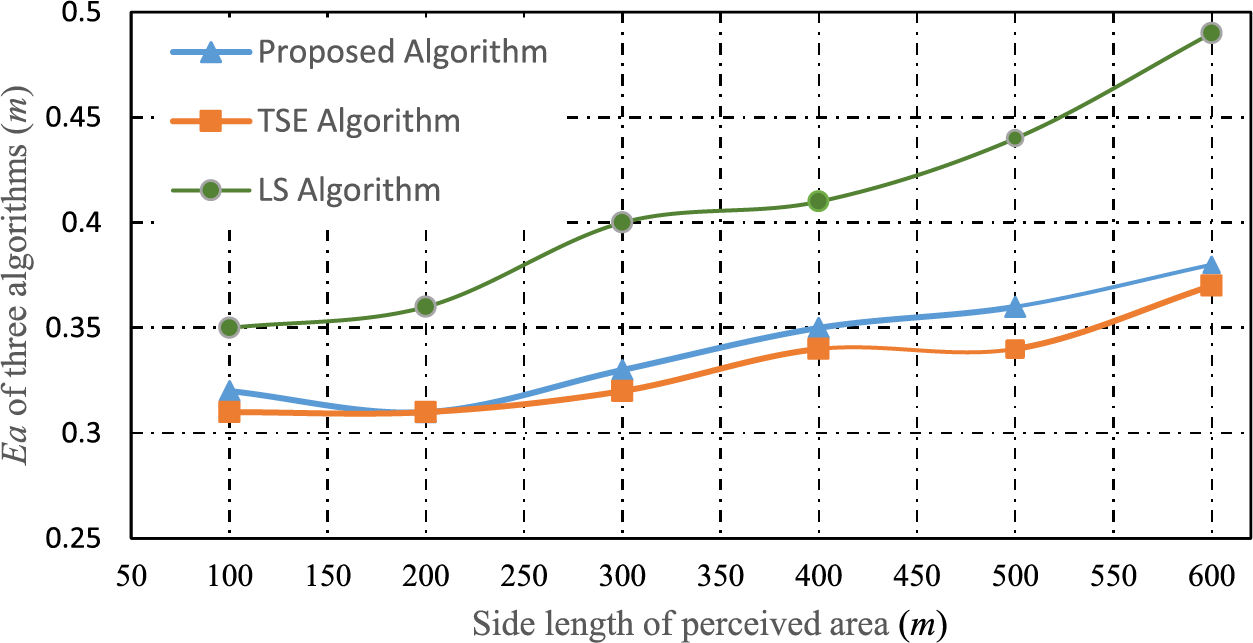
Figure 4: Effect of the perceived region size on the average localization error

From the positioning performance curve in Fig. 4, it can be seen that as the edge length of the perception area continues to increase, i.e., the network size increases, the average positioning error of the three algorithms gradually increases. However, the positioning error of the proposed algorithm is close to the TSE algorithm and lower than the LS algorithm. The reason is that as the edge length of the perception area increases, the network size continues to increase, and the number of nodes in the network that need to be located increases. The measurement error and cumulative error of the positioning algorithm also increase, resulting in an overall increase in positioning error and an increase in average positioning error.

4.5 Interrelation between the Positioning Precision and the Number of Nodes

Let’s study the effect of increasing the number of nodes on the average positioning error when the reference node value is n=20. Here, the positioning experiment environment is still a 2-D square area of 200 m × 200 m. The network node numbers change from 100 to 400, and its impact on the average positioning error is shown in Fig. 5.

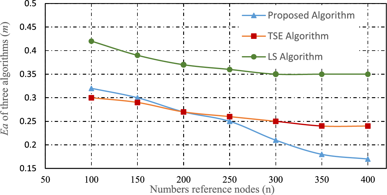
Figure 5: Effect of the number of network nodes on the average localization error

From the average positioning error curve in Fig. 5, it can be seen that when the number of reference nodes is fixed and unchanged, as the number of nodes to be located in the fixed network positioning area increases, the positioning performance of all three algorithms improves. Comparatively speaking, the positioning error of the proposed algorithm decreases rapidly and is much smaller than that of the LS algorithm. The reason is that the former not only adopts distance measurement error correction but also implements the measure of selecting optimal reference nodes when the network node density increases and the number of reference nodes that can participate in positioning increases. In addition, the iterative refinement algorithm further improves the positioning accuracy.

4.6 Interrelation between the Positioning Precision and the RSSI Ranging Error

Finally, we study the interrelation between RSSI ranging error and positioning error. Setting the number of reference nodes to 20, and the total number of nodes to be located in the network to 400. The impact of RSSI ranging error on average positioning error is shown in Fig. 6.

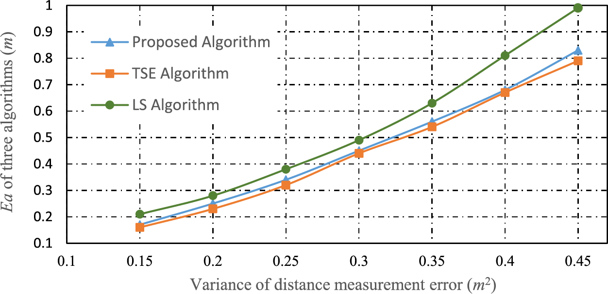
Figure 6: Effect of the RSSI ranging error on the average localization error

From the trend of the positioning performance curve in Fig. 6, it can be seen that under the same number of nodes, as the variance of RSSI distance measurement error gradually increases, the average positioning error of all three algorithms increases. But the average positioning error of the proposed algorithm increases much faster than the LS algorithm, and at the same RSSI distance measurement error variance, the proposed algorithm’s positioning accuracy is always better than the LS algorithm and the positioning results are also more stable. It can be seen that the dynamic acquisition technology using power-fading factor and weighted ranging relative error correction can effectively and quickly reduce positioning errors and improve positioning performance.

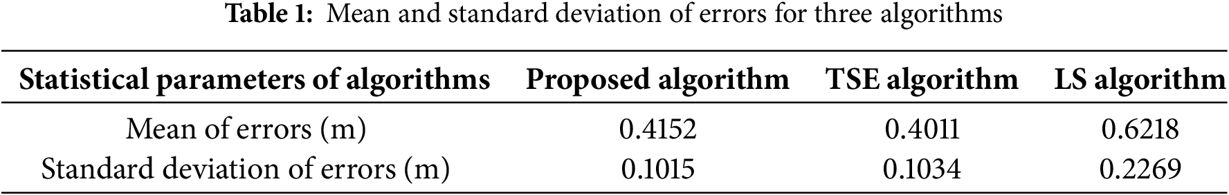
In order to provide a statistical analysis of the positioning results of the algorithm proposed in this article, we calculated the statistical parameters of three algorithms, such as the mean error and standard deviation indicators. The simulation scenario is described in Section 4.6, and the mean and standard deviation of the errors of the three algorithms are shown in Table 1. It can be seen that the algorithm proposed in this article uses relative distance error coefficient for RSSI ranging correction, and then uses reference node coordinate error to correct the position coordinates of the node to be located. Therefore, the mean error of the positioning result of the proposed algorithm is close to the TSE algorithm, but much smaller than the LS algorithm. The standard deviation of the proposed algorithm has always been maintained at a low level, that is, lower than the TSE algorithm and the LS algorithm.

4.7 Computation Time

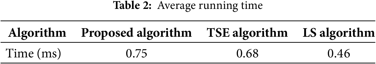
In order to analyze and compare the complexity of the algorithm proposed in this article with other algorithms, we calculated the average running time of several algorithms. The data simulation processing platform consists of a PC with the following parameters: Intel (R) Core (TM) i7-8700 CPU @ 3.20 GHz, 16.0 GB RAM, 64-bit operating system based on ×64 processor, and MATLAB 2019A as the software testing environment for executing the simulation process. The simulation scenario is described in Section 4.6, and the running time of each algorithm positioning is shown in Table 2. The algorithm proposed in this article introduces collaborative positioning, upgrading the already located nodes to reference nodes and partaking in the positioning of other nodes. Finally, the Taylor series least squares iterative refinement algorithm is used to obtain more accurate position coordinates of network nodes, but at the same time, it also comes at a slightly higher cost, namely increased running time. Under the same positioning environment and operating parameter conditions, it can be seen from the comparison of the running time of various algorithms that the algorithm proposed in this paper, the proposed algorithm, has a slightly higher running time in estimating the position of the node to be located than the TSE algorithm and LS algorithm.

5  Conclusion

On account of the dynamic acquisition technology of power fading factor using RSSI ranging and weighted relative error correction, this article proposes a sensor network supervised positioning algorithm based on coordinate error correction and Taylor series least squares iterative optimization. Through an in-depth study of the RSSI ranging principle and the demands of the positioning system, we applied the ranging algorithm of dynamically obtaining the power-fading factor, and used the relative distance error coefficient of the reference node in the positioning area to conduct the RSSI distance correction. After obtaining the solution of the least square positioning algorithm, we then use the location deviation of the reference nodes to revise the position coordinates of the nodes to be located, and further improve the positioning accuracy. Finally, we used the algorithm of Taylor series least squares loop iterative refinement to obtain the accurate position coordinate information of the network nodes. In the localization based on the RSSI ranging principle, there are always some nodes that become unloadable nodes due to various reasons (such as distribution outside the localization range, receiving insufficient information, etc.). By introducing collaborative positioning, the located nodes are upgraded to reference nodes to partake in the positioning of other nodes, which improves the coverage of positioning, so it can adapt to a wider range of scenarios and environments that are more complex. Simulation shows that the positioning precision of the algorithm in this article can meet the application demand of large-scale wireless sensor network systems, with low computational complexity and communication overhead. It can effectively resist noise interference and has good performance in both positioning precision and cost power consumption.

This article adopts a collaborative optimization method to solve the problem of improving the positioning accuracy of sensor networks. However, with the increasing complexity of algorithms caused by environmental changes and interference, sensor network positioning systems still face many unresolved issues. Therefore, the next step of this article will consider the assumptions of expanding network topology or node capabilities, the uncertainty of sensor positions caused by dynamic networks, and the application of collaborative and optimization methods to 3D extended localization and mobile sensor network localization problems. At the same time, direct measurements between nodes are used for collaborative positioning, and estimation theory is applied for evaluation to further reduce various system and measurement errors in the positioning process, in order to improve positioning quality such as positioning accuracy and robustness.

Acknowledgment: The authors would like to thank the editors of CMC and anonymous reviewers for their time and for reviewing this manuscript.

Funding Statement: National Natural Science Foundation of China, grant number 62205120, funded this research.

Author Contributions: The authors confirm contribution to the paper as follows: study conception and design: Bo Chang, Xinrong Zhang; data collection: Bo Chang, Xinrong Zhang; analysis and interpretation of results: Bo Chang, Xinrong Zhang; draft manuscript preparation: Bo Chang. All authors reviewed the results and approved the final version of the manuscript.

Availability of Data and Materials: The authors confirm that the data supporting the findings of this study are available within the article.

Ethics Approval: Not applicable.

Conflicts of Interest: The authors declare no conflicts of interest to report regarding the present study.

References

1. Li X, Pang H, Li G, Jiang J, Zhang H, Gu C, et al. Wireless positioning: technologies, applications, challenges, and future development trends. Comput Model Eng Sci. 2024;139(2):1135–66. doi:10.32604/cmes.2023.031534. [Google Scholar] [CrossRef]

2. Rani S, AnjuN, Sangwan A, Kumar K, Nisar K, Soomro T, et al. A review and analysis of localization techniques in underwater wireless sensor networks. Comput Mater Contin. 2023;75(3):5697–715. doi:10.32604/cmc.2023.033007. [Google Scholar] [CrossRef]

3. Mani R, Rios-Navarro A, Sevillano-Ramos JL, Liouane N. Improved 3D localization algorithm for large scale wireless sensor networks. Wirel Netw. 2024;30(6):5503–18. doi:10.1007/s11276-023-03265-0. [Google Scholar] [CrossRef]

4. Prashar D, Jyoti K. Distance error correction based hop localization algorithm for wireless sensor network. Wirel Pers Commun. 2019;106(3):1465–88. doi:10.1007/s11277-019-06225-0. [Google Scholar] [CrossRef]

5. Annepu V, Rajesh A. Implementation of self-adaptive mutation factor and crossover probability based differential evolution algorithm for node localization in wireless sensor networks. Evol Intell. 2019;12(3):469–78. doi:10.1007/s12065-019-00239-0. [Google Scholar] [CrossRef]

6. Cheng M-M, Zhang J, Wang D-G, Tan W, Yang J. A localization algorithm based on improved water flow optimizer and max-similarity path for 3-D heterogeneous wireless sensor networks. IEEE Sens J. 2023;23(12):13774–88. doi:10.1109/JSEN.2023.3271820. [Google Scholar] [CrossRef]

7. Kaur A, Kumar P, Gupta GP. A weighted centroid localization algorithm for randomly deployed wireless sensor networks. J King Saud Univ-Comput Inform. 2019;31(1):82–91. doi:10.1016/j.jksuci.2017.01.007. [Google Scholar] [CrossRef]

8. Ullah I, Shen Y, Su X, Esposito C, Choi C. A localization based on unscented Kalman filter and particle filter localization algorithms. IEEE Access. 2020;8:2233–46. doi:10.1109/ACCESS.2019.2961740. [Google Scholar] [CrossRef]

9. Yan J, Ban H, Luo X, Zhao H, Guan X. Joint localization and tracking design for AUV with asynchronous clocks and state disturbances. IEEE Trans Veh Technol. 2019;68(5):4707–20. doi:10.1109/TVT.2019.2903212. [Google Scholar] [CrossRef]

10. Luomala J, Hakala I. Analysis and evaluation of adaptive rssi-based ranging in outdoor wireless sensor networks. Ad Hoc Netw. 2019;87(4):100–12. doi:10.1016/j.adhoc.2018.10.004. [Google Scholar] [CrossRef]

11. Wu S, Zhang S, Huang D. A TOA­ based localization algorithm with simultaneous NLOS mitigation and synchronization error elimination. IEEE Sens Lett. 2019;3(3):1–4. doi:10.1109/LSENS.2019.2955125. [Google Scholar] [CrossRef]

12. Kwon Y, Kwon K. RSS Ranging based indoor localization in ultra-low power wireless network. AEU-Int Electron Commun. 2019;104:108–18. [Google Scholar]

13. Dai W, Shen Y, Win MZ. A computational geometry framework for efficient network localization. IEEE Trans Inf Theory. 2018;64(2):1317–39. doi:10.1109/TIT.2017.2674679. [Google Scholar] [CrossRef]

14. Xue W, Hua X, Li Q, Yu K, Qiu W, Zhou B, et al. A new weighted algorithm based on the uneven spatial resolution of RSSI for indoor localization. IEEE Access. 2018;6:26588–95. doi:10.1109/ACCESS.2018.2837018. [Google Scholar] [CrossRef]

15. Xia W, Liu W. Distributed adaptive direct position determination of emitters in sensor networks. Signal Process. 2016;123(4):100–11. doi:10.1016/j.sigpro.2016.01.002. [Google Scholar] [CrossRef]

16. Sathish K, Chinthaginjala R, Kim W, Rajesh A, Corchado JM, Abbas M. Underwater wireless sensor networks with RSSI-based advanced efficiency-driven localization and unprecedented accuracy. Sensors. 2023;23(15):6973–87. doi:10.3390/s23156973. [Google Scholar] [PubMed] [CrossRef]

17. Kwok C, Fox D, Meila M. Real-time particle filters. Proc IEEE. 2004;92(3):469–84. doi:10.1109/JPROC.2003.823144. [Google Scholar] [CrossRef]

18. Aziz MAE. Source localization using TDOA and FDOA measurements based on modified cuckoo search algorithm. Wirel Netw. 2017;23(2):1–9. [Google Scholar]

19. Nguyen HD, Wood IA. A block successive lower-bound maximization algorithm for the maximum pseudo-likelihood estimation of fully visible boltzmann machines. Neural Comput. 2016;28(3):485–92. doi:10.1162/NECO_a_00813. [Google Scholar] [PubMed] [CrossRef]

20. Van Nguyen T, Jeong Y, Shin H, Win MZ. Least square cooperative localization. IEEE Trans Veh Technol. 2015;64(4):1318–30. doi:10.1109/TVT.2015.2398874. [Google Scholar] [CrossRef]

21. Khan MW, Salman N, Kemp AH. Optimised hybrid localization with cooperation in wireless sensor networks. Signal Process. 2017;11(3):341–8. [Google Scholar]

22. Wang ZF, Zhang H, Lu TT, Gulliver TA. Cooperative RSS-based localization in wireless sensor networks using relative error estimation and semidefinite programming. IEEE Trans Veh Technol. 2019;68(1):483–97. doi:10.1109/TVT.2018.2880991. [Google Scholar] [CrossRef]

23. Li H, Trocan M, Galayko D. Virtual fingerprint and two-way ranging-based Bluetooth 3D indoor positioning with RSSI difference and distance ratio. J Electromagn Waves Appl. 2019;33(16):2155–74. doi:10.1080/09205071.2019.1667268. [Google Scholar] [CrossRef]

24. Ren Q, Zhang Y, Nikolaidis I, Li J, Pan Y. RSSI quantization and genetic algorithm based localization in wireless sensor networks. Ad Hoc Netw. 2020;107:102255. doi:10.1016/j.adhoc.2020.102255. [Google Scholar] [CrossRef]

25. Chang B, Zhang X, Bian H. An accurate cooperative localization algorithm based on RSS model and error correction in wireless sensor networks. Electronics. 2024;13(11):2131. doi:10.3390/electronics13112131. [Google Scholar] [CrossRef]