Graph Similarity Learning Based on Learnable Augmentation and Multi-Level Contrastive Learning

1  Introduction

Graph similarity learning aims to compute the similarity between two graphs, which is crucial for various downstream applications, including graph-based database similarity search [1] and software homology detection [2].

Existing graph similarity learning methods mainly include traditional definition-based methods [3] and graph deep learning-based methods. Definition-based methods calculate the distance between graph pairs solely based on structural features, neglecting the rich attribute information within graphs and thereby limiting their applicability. In contrast, graph deep learning-based methods, which consider both structural and attribute features, have emerged as the mainstream in current research.

Graph similarity learning methods based on graph deep learning typically use Graph Neural Networks (GNNs), which require labeled data and are thus categorized as supervised learning. To address the high cost of manual labeling, unsupervised methods, particularly contrastive learning, have gained traction [4,5]. Contrastive learning learns representations by maximizing feature consistency across different augmented views [6] and has demonstrated exceptional performance in computer vision tasks [7]. Despite its success, applying contrastive learning to graph similarity learning presents several challenges.

Firstly, classic image augmentation techniques like grayscaling, rotation, and blurring preserve image semantics, as illustrated in Fig. 1a, but applying similar methods to graphs may alter their semantics. For instance, random edge disconnection can significantly affect graph properties, as shown in Fig. 1b, where disconnecting an edge increases the distance between communities. In Fig. 1c, the graph’s structure changes from the choice to a sequential one. This difference arises from the distinction between Euclidean (image) and non-Euclidean (graph) data, where images maintain spatial relationships, but graphs require preserving both semantic and structural consistency. In graph similarity learning, disruptions caused by augmentation can lead to issues like label inconsistency, where the augmented graph no longer aligns with the original labels, error propagation, which introduces biases in similarity computation, and reduced generalization, leading to unstable predictions on unseen data. Thus, designing effective graph augmentation strategies requires preserving the critical semantic and structural information of the original graph.

Figure 1: (a), (b), and (c) illustrate the differences between Euclidean and non-Euclidean structures during augmentation, while (d) shows significant substructures within graph structures

Secondly, existing research often compares graph pairs solely at the node level, overlooking substructures that capture the mesoscopic information of graphs. For example, in Fig. 1d, two compounds share the same substructure, which may result in similar properties. However, node-based graph similarity learning methods fail to identify these substructures, thereby missing critical local similarities.

This limitation stems from the inherent narrow focus of single-level approaches, which primarily analyze node-to-node relationships without considering hierarchical or multi-level graph features. Substructures, such as motifs or communities, represent mesoscopic patterns that capture intermediate relationships between local nodes and the global structure. Neglecting these patterns may lead to incomplete or misleading similarity scores.

Incorporating these hierarchical representations into graph similarity learning frameworks could enhance their ability to accurately capture and compare graphs across diverse domains. Effectively addressing these challenges remains a critical area for further research.

This paper introduces GSLM, a graph similarity learning model based on learnable augmentation and multi-level contrastive learning, to address the abovementioned issues. Augmented views are generated for each graph by modifying attributes and structure, with subgraphs enhancing the contrastive hierarchy. Node-level and subgraph-level representations are learned for each view, followed by joint contrastive training. Graph similarity scores are computed for downstream tasks. Evaluations on eight datasets show that GSLM outperforms baseline methods in both graph classification and regression tasks. The main contributions include:

(1) A novel unsupervised graph similarity learning model is proposed, effectively calculating the similarity between graph pairs through learnable augmentation and multi-level contrastive learning.

(2) Learnable augmentation methods and multi-level contrastive strategies are proposed for attributes and structure. The augmentation method generates augmented views of the original graph while preserving critical information. The multi-level contrastive strategy complements node-level contrast with subgraph-level contrast, enriching the model’s contrastive levels. Learnability refers to the model’s ability to select relevant attributes and structures for augmented views based on their importance.

(3) Comprehensive experiments were conducted on two regression and six classification datasets, demonstrating the effectiveness of the proposed model.

The remainder of this paper is organized as follows: Section 2 introduces related work; Section 3 presents the problem definition; Section 4 presents the proposed unsupervised graph similarity learning method, GSLM; Section 5 presents the experimental results and comparisons with baseline methods, validating the effectiveness of the proposed method; Section 6 concludes the paper and discusses future work.

2  Related Work

Research methods for graph similarity learning can be divided into traditional and GNN-based methods.

2.1 Traditional Methods

Among various definitions of graph similarity, Graph Edit Distance (GED) and Maximum Common Subgraph (MCS) [8] are two domain-agnostic graph similarity measures. Traditional graph similarity learning methods generally rely on GED or MCS as the similarity measure. However, calculating GED or MCS is an NP (non-deterministic polynomial)-hard problem [8].

Traditional methods can be divided into two categories: the first category computes exact values [9,10]. Although exact similarity measures can better understand the relationships between graphs, the time complexity of exact graph similarity computation is exponential, which is impractical in real-world applications. The second category computes approximate values [11]. While this approach saves time, its time complexity still reaches polynomial or even exponential levels. Additionally, traditional algorithms primarily focus on the graph’s topological structure, ignoring the attribute information contained within the graph (e.g., node features, edge features).

2.2 GNN-Based Methods

Recent graph similarity learning methods can be divided into two major categories: supervised methods [12–16] and unsupervised methods [4,5,17]. The former fully utilizes labels to obtain graph embeddings, ultimately used to calculate graph similarity. However, in real-world scenarios, labeled data is often difficult to obtain, and the quality of labeled data varies. Therefore, unsupervised graph similarity learning methods have gained attention. Nonetheless, previous methods often damage the attributes and structural features of graphs during augmentation, negatively impacting unsupervised graph similarity learning tasks.

Previous studies overlooked the impact of random augmentation on graph similarity learning tasks, which could alter labels and lower similarity scores for initially similar graphs. They also focused on node-level comparisons, neglecting multi-level and local similarities. This paper addresses these issues by incorporating attribute and structural augmentation to preserve label-invariant information and introducing subgraph-level contrastive learning to model mesoscopic similarities and enhance contrastive levels.

3  Problem Definition

A graph is represented as G=(V,E,X,A), where V={v1,v2,…,vN} is the set of nodes and N is the total number of nodes; E is the set of edges, where eij={vi,vj}∈E represents the edge between nodes vi and vj. If there is an edge between vi and vj, then eij=1 otherwise, eij=0. A∈RN×N is the adjacency matrix of the graph, and aij=eij. X={x1,x2,…,xN}∈RN×D is the attribute matrix, and D represents the dimension of the attributes.

Given two graphs G1 and G2, the task of graph similarity learning is to compute a similarity score y to measure the similarity between G1 and G2.

4  GSLM Model

The proposed GSLM model consists of four modules: 1. Input module; 2. Graph augmentation module: This module generates different augmented views of the original graphs based on attributes and topology and samples appropriate subgraphs; 3. Multi-level contrastive learning module: This module computes the node and subgraph embeddings and conducts joint training; 4. Similarity computation module: Based on different downstream tasks, graph-level representations are processed to obtain the final similarity scores. As shown in Fig. 2, the multi-level contrastive learning module has many details, which will be elaborated on in Section 4.3.

Figure 2: The architecture of GSLM

The following sections introduce the specific content of each module in the model.

4.1 Input Module

The input to the graph similarity learning task is a pair of graphs, denoted as G1=(V1,E1,X1,A1) and G2=(V2,E2,X2,A2).

4.2 Graph Augmentation Module

Traditional augmentation methods, such as random edge disconnection or node feature perturbation, often rely on predefined rules and lack adaptability to specific graph structures. This can result in semantic and structural inconsistencies. In contrast, learnable augmentation dynamically adapts to the data and task by leveraging trainable modules that assess the importance of graph components (nodes and edges). Learnable augmentation incorporates feedback from the model’s loss function, preserving similarity scores in graph similarity learning. The approach allows for targeted modifications that preserve critical information while minimizing unintended disruptions.

This module is divided into graph-level augmentation (attribute augmentation layer and structural augmentation layer) and subgraph-level augmentation (subgraph selection layer). Learnable methods are used to obtain corresponding attribute-augmented and structure-augmented views for graph-level augmentation. For subgraph-level augmentation, a subgraph augmentation scheme is designed to enrich the contrastive levels.

4.2.1 Attribute Augmentation Layer

Previous contrastive learning approaches in graph similarity often randomly masked node attributes, which could result in losing critical semantic information. To address this, less essential attributes should be masked during augmentation to preserve important information from the original graph.

Some studies use statistical metrics, such as variance and information gain to evaluate feature importance, but these methods are not robust, and lack flexibility. A better approach is needed, where the model can automatically evaluate and select important attributes. Inspired by [18], the Gumbel-Softmax method enables end-to-end training, dynamic feature selection, and improved model robustness by computing parameters and gradients automatically.

Specifically, taking the original graph features X as input, a multi-layer perceptron (MLP) is used to generate a, which measures the importance of each node’s features. The Gumbel-Softmax method is then applied to reparameterize a to obtain a one-hot vector f. Finally, an augmentation function is used to obtain the final augmented features:

a=MLP(X)(1)

f=GumbelSoftmax(a)(2)

Xaug=Aug1(X,f)(3)

where the MLP represents the multi-layer perceptron, a represents the probability of selecting whether to mask or retain the original feature, f is the one-hot vector obtained through Gumbel-Softmax sampling, and Xaug is the augmented feature after being processed by the augmentation function Aug1().

4.2.2 Structural Augmentation Layer

Previous methods used random edge deletion for structural augmentation, which can lose important information and alter graph labels. To preserve more information, edges should be weighted by importance. While edge betweenness centrality is one approach, it’s computationally expensive and ignores attributes. The Graph Attention Network (GAT) adapts edge weights through self-attention, incorporating both structural and attribute information, and is used to guide edge deletion during structural augmentation.

Specifically, taking the original graph’s topology A and features X as input, the attention scores for edges are calculated, which are then used as the standard for topology augmentation, resulting in the augmented topology:

αij=exp⁡(LeakyReLU(a→T[Wxi→||Wxj→]))∑k=Niexp⁡(LeakyReLU(a→T[Wxi→||Wxk→]))(4)

Aaug=Aug2(αij,A)(5)

where the αij represents the attention score between node i and node j, a→T and W are shared learnable parameters, || denotes concatenation, and LeakyReLU is the activation function. Ni represents the neighbors of node i, and SoftMax is used to normalize the attention scores. The augmented adjacency matrix is then obtained through an augmentation function.

4.2.3 Subgraph Selection Layer

Previous work used node-level information for contrastive learning, neglecting the impact of local structures. This can lead to the loss of local similarities between graph pairs. Therefore, both subgraph-level information and node-level information are incorporated.

For subgraph selection, research [19] has demonstrated that larger subgraphs tend to have higher semantic similarity, making them more informative and suitable for contrastive learning. Inspired by these findings, a biased random walk (BRW) approach is used to select large subgraphs, with the selected subgraph denoted as Gsub=ϕ(G), where ϕ represents the biased random walk method. The BRW method allows for the sampling of large, structurally coherent subgraphs by prioritizing nodes and edges based on their connectivity and importance, thus preserving local structures and meaningful graph semantics. The positive example is the pair of subgraphs generated from the original graph, while the negative example is subgraphs generated from other graphs. This strategy ensures that the contrastive learning framework captures both local and global similarities by leveraging subgraph-level information in addition to node-level embeddings.

By integrating subgraph-level information through BRW, the proposed method enriches the hierarchical representation of graphs and improves the model’s ability to differentiate between graph pairs with subtle structural and semantic differences.

4.3 Multi-Level Contrastive Learning Module

Fig. 3 shows the multi-level contrastive learning module, which includes four layers: the node embedding layer, the node interaction layer, the subgraph embedding layer, and the contrastive learning layer.

Figure 3: Multi-level contrastive learning module

From an information-theoretic perspective, multi-level representations maximize the mutual information between different scales of graph features, enabling the model to capture richer and more meaningful similarities. Additionally, leveraging multi-level features increases the diversity of positive and negative samples in contrastive learning, leading to more robust and generalizable graph similarity measures.

4.3.1 Node Embedding Layer

This layer generates initial node-level embeddings for the original graph, its augmented views, its augmented views, and subgraphs using a Graph Convolutional Network (GCN), which effectively captures local structural and attribute information. These initial embeddings serve as input to the subsequent node interaction layer, which incorporates an attention mechanism to model the interactions between nodes across the augmented views and original views. To better capture subtle differences between the original graph and its augmented views, a Siamese network structure is used in combination with the GCN:

Hl=σ(A~Hl−1Wl−1)(6)

where the H represents the node embeddings, l denotes the number of embedding layers. A~ is the normalized Laplacian matrix; W denotes the training weight matrix, and σ denotes the sigmoid function.

4.3.2 Node Interaction Layer

Inspired by graph contrastive learning, we aim to increase the similarity between positive examples (same nodes in different views) and decrease it for negative examples (other nodes). Suppose the embedding of node i is denoted as hi, and the embedding of node j is denoted as hj. The similarity between them is defined as:

sim(hi,hj)=cos⁡(hi,hj)(7)

As shown in Fig. 3, to maximize the consistency between nodes across different views and learn node correspondences between different graphs, we first calculate the similarity between augmented views, then increase the similarity between augmented views and the similarity across different graphs:

h~iaug1=hiaug1⊕∑j∈G1aug2sim(hiaug1,hjaug2)hjaug2(8)

h¯iaug1=hi⊕∑u∈G2aug1sim(hi,h~uaug1)h~uaug1⊕∑v∈G2aug2sim(hi,h~vaug2)h~vaug2(9)

where i and j denote nodes in the original graph or augmented views of G1, and u and v denote nodes in the original graph or augmented views of G2. In Eq. (8), the similarity between augmented views of the same graph is first computed, and the similarity within augmented views is considered a weight in the node representation. The notation G1aug2 represents the second augmented view G1 and ⊕ denotes the concatenation operation. Next, the interaction between different graphs is considered. As shown in Eq. (9), the two augmented views of G2 are compared with the embedding vector of G1 to calculate the similarity, ultimately obtaining the embedding of node h¯iaug1 in the first augmented view of G1. Here, G2aug1 and G2aug2 represent the two augmented views of G2.

4.3.3 Subgraph Embedding Layer

After obtaining the node-level representations of the subgraphs, a pooling function is applied to obtain the subgraph representation. In this case, average pooling is used as the pooling function, and the subgraph representation is obtained as follows:

s=Avg(hi,i∈Gsub)(10)

where Avg() represents average pooling.

4.3.4 Contrastive Learning Layer

After obtaining the node and subgraph embeddings, InfoNCE [6] is used to maximize the similarity between positive examples and minimize the similarity between negative examples. Consequently, the loss function for node representations within a graph is defined as follows:

loss(h¯iaug1,h¯jaug2)=−log⁡sim(h¯iaug1,h¯jaug2)sim(h¯iaug1,h¯jaug2)+∑k=1Nsim(h¯iaug1,h¯k)(11)

where i and j denote a pair of positive examples, and N represents the number of negative examples. Since the final goal is to calculate the similarity between two graphs, the node-level loss function is defined as:

Lnode=12(loss(h¯iaug1,h¯jaug2)+loss(h¯uaug1,h¯vaug2))(12)

Since previous unsupervised graph similarity learning methods considered contrastive learning only at the node level and ignored local information within the graph, subgraph-level information is incorporated into the training process to model richer multi-level information. Similar to the node-level loss function, the subgraph-level loss function is defined as follows:

Lsub=12(loss(s1sub1,s1sub2)+loss(s2sub1,s2sub2))(13)

Finally, the node-level and subgraph-level losses are jointly trained, and the final loss is:

ℓ=Lnode+Lsub(14)

4.4 Similarity Computation Module

After obtaining the node representations of the graph, the graph-level representation is computed for similarity scoring. As prior work [15] shows that the BiLSTM (Bi-directional Long Short-Term Memory) aggregator offers superior expressive power, it is used to derive the graph-level embedding Z:

Z=BiLSTM(hi),i∈G(15)

where the BiLSTM takes the randomly permuted node embeddings as input and concatenates the final hidden vectors from both directions of the LSTM (Long Short-Term Memory) as the graph representation Z.

For graph classification task, directly computing the cosine similarity between two graph-level embeddings is desirable. Therefore, cosine similarity is used to calculate the similarity between the graph-level embeddings:

y=cos⁡(Z1,Z2)(16)

For graph regression task, the predicted result in a graph regression task is continuous and needs to be normalized within the range of [0,1]. To achieve this, the two graph-level embeddings are first concatenated, then projected onto a scalar, and finally passed through an activation function to constrain the similarity score within the desired range, as shown in the following equation:

y=σ(MLP(Z1⊕Z2))(17)

where σ is the sigmoid function, used to normalize the similarity score, and ⊕ denotes the concatenation operation.

5  Experiments

To validate the effectiveness of the proposed model, experiments were conducted on both graph classification and graph regression tasks. Three groups of experiments were designed to address the following questions:

1. Does the proposed model outperform previous models in terms of performance?

2. How does the choice of different parameters in the model affect similarity learning?

3. Does the proposed learnable augmentation positively impact similarity learning?

5.1 Experimental Data and Evaluation Metrics

5.1.1 Experimental Data

The datasets used in the experiments are described in Table 1 [15].

The model was evaluated on eight public datasets. For graph regression, two benchmark datasets, Aids700nef and Linux1000, were used, split into 60%, 20%, and 20% for training, validation, and testing. For graph classification, six datasets were generated using FFmpeg and OpenSSL. In the supervised method, the dataset split was 10%, 10%, and 80%, while in the unsupervised method, it was 80%, 10%, and 10%.

5.1.2 Evaluation Metrics

For the graph regression task, the primary evaluation metric used was Mean Squared Error (MSE), which measures the difference between the model’s predicted and true values. A smaller MSE indicates better model performance. Additionally, Spearman’s rank correlation coefficient ρ [13], Kendall’s rank correlation coefficient τ [15], and precision at k (p@k) were also used. The rank correlation coefficients ρ and Kendall’s coefficient τ measure the agreement between the predicted and actual ranking results, while p@k indicates the proportion of correctly predicted relevant results out of all returned results. Higher values of these metrics indicate better model performance.

For the graph classification task, the area under the ROC (Receiver Operating Characteristic) curve (AUC) was used as the evaluation metric. AUC reflects the model’s discriminative ability, with a value closer to 1 indicating better classification performance.

5.2 Baseline Algorithms and Parameter Settings

The proposed model was compared with two supervised methods (GCN and GIN (Graph lsomorphism Network)), which focus on feature aggregation and graph isomorphism handling, and three unsupervised methods (DGI (Deep Graph Infomax), GRACE (GRAph Contrastive rEpresentation learning), and CGMN (Contrastive Graph Matching Network)), which utilize contrastive learning for representation learning and graph similarity computation.

The graph regression and classification tasks are treated as downstream tasks. The learning rate was set to 0.0001, with a three-layer GCN encoder and dimensions of 100 for the graph encoder, projection, and prediction layers. The same settings (e.g., dataset splits and learning rate) were used for the graph regression task for the supervised baselines. For the unsupervised baselines, 1% of the true value’s MSE loss was used for fine-tuning. In the graph classification task, the supervised models were trained using the same method as in the graph regression task. In contrast, the unsupervised baselines used their self-contained losses for graph representation learning. All experiments were repeated five times, and the mean and standard deviation of the results were reported, with the best results highlighted in bold.

5.3 Baseline Comparison

To address question 1, the following baseline experiments were designed, with the results shown in Tables 2 and 3.

As shown in Tables 2 and 3, the proposed model generally outperforms the baseline models in both graph regression and classification tasks. On the one hand, traditional supervised graph representation learning models, such as GCN and GIN, lack specific modules designed for graph similarity learning tasks. This leads to poor performance in graph similarity calculations, as they overlook the interaction information between graph pairs. On the other hand, previous contrastive learning methods did not address the issue of augmentation randomness, which destroys the label information of the original graph. Additionally, they only performed node-level contrast while ignoring the modeling of local similarity in graph pairs, resulting in suboptimal performance.

As dataset size grows, the model’s performance slightly declines due to increased graph complexity and sparsity but remains superior to baselines. It scales effectively, with minimal performance loss and slight computation time increases.

To further evaluate the effectiveness of the proposed model, we performed a visualization of graph embeddings for both the proposed model and the baseline methods on Linux1000. This visualization aligns with the superior performance observed in Tables 2 and 3, where the proposed model outperformed baseline methods. The results are shown in Fig. 4.

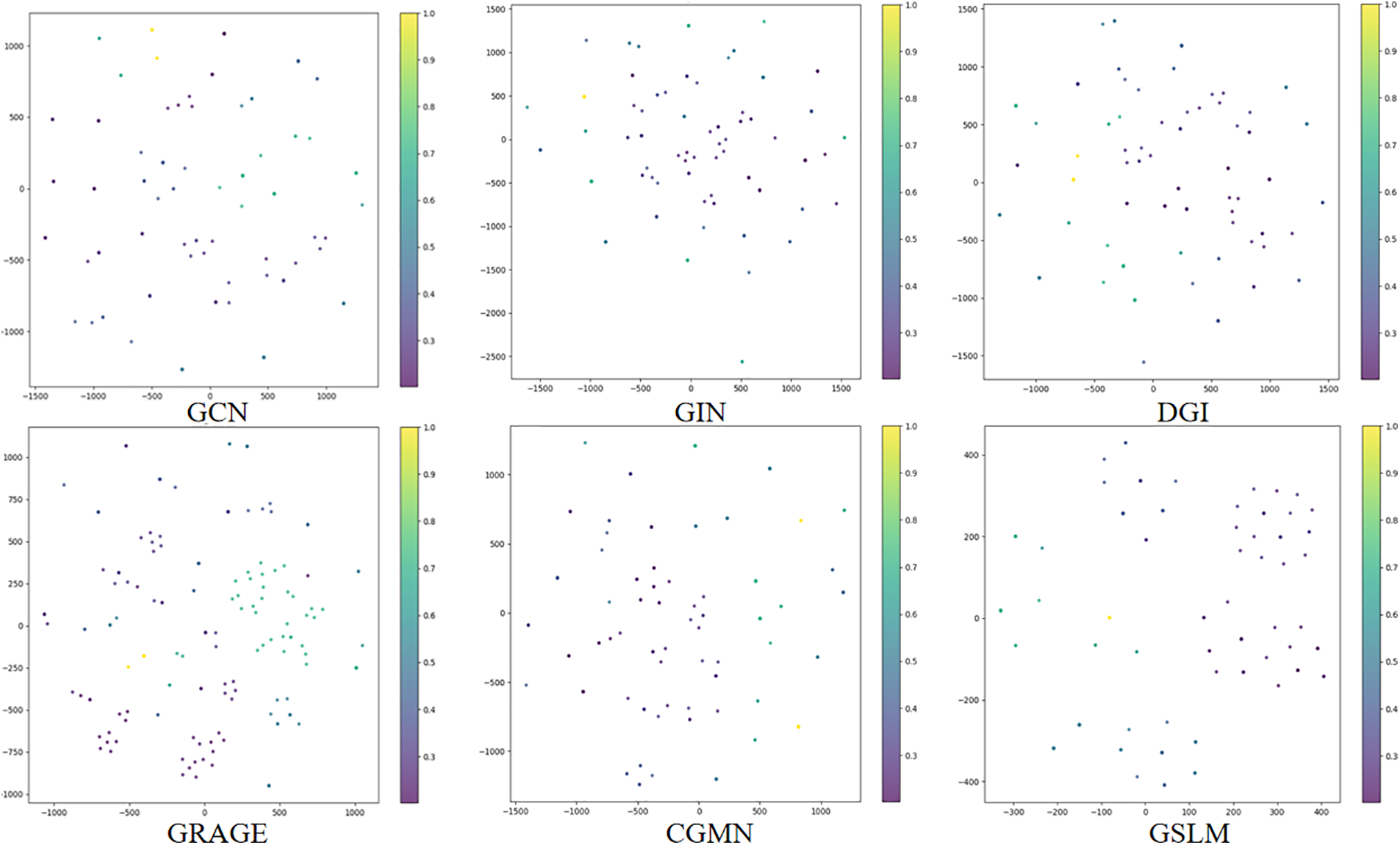
Figure 4: Visualization of graph embeddings generated by different models on Linux1000

5.4 Parameter Sensitivity Analysis

To address question 2, the following experiments were conducted to determine the optimal parameters, including the number of GNN layers l, learning rate lr, and the dimension of the final layer d:

(1) GNN Layers: The experiments show that the model performs best when l=3. On the one hand, when the number of encoder layers is too low, the model may not learn sufficient features and structural information from the graph, resulting in poor performance. On the other hand, when the number of encoder layers is too high, overfitting may occur, leading to poor performance. The results are shown in Fig. 5.

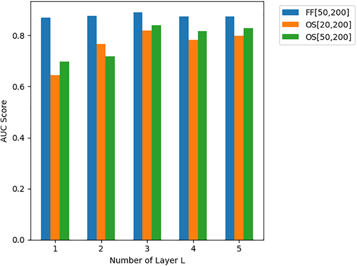
Figure 5: Hyperparameter study on GNN layers

(2) Learning Rate: The experiments demonstrate that the model performs best when lr=0.0001. The results are shown in Fig. 6.

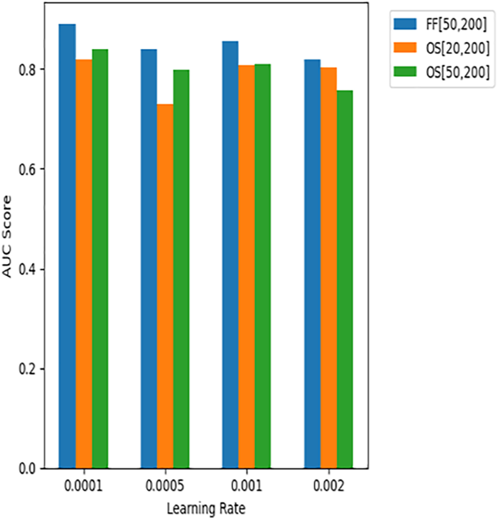
Figure 6: Hyperparameter study on learning rate

(3) Final Layer Dimension: Considering the efficiency of the encoder, the dimension of the final layer was set between 50 and 150, with experiments showing that the model performs best when d=100. The results are shown in Fig. 7.

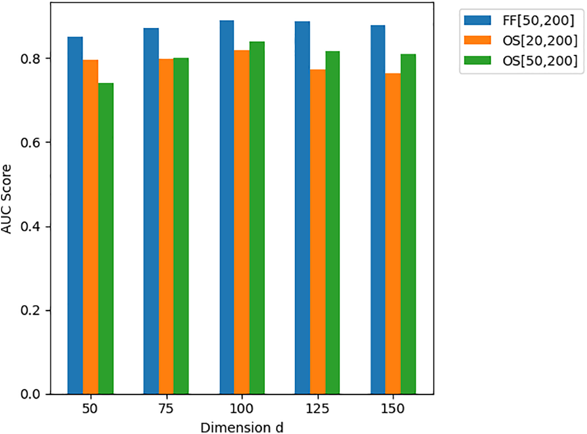
Figure 7: Hyperparameter experiment on final layer dimension

5.5 Ablation Study

To address question 3, the effects of adaptive augmentation strategies and subgraph-level contrast were investigated. “w/o” indicates module removal, “SA” is the structural augmentation module, “FA” is the feature augmentation module, and “Subgraph-Level Contrast” refers to contrast loss. Results are in Tables 4 and 5.

Tables 4 and 5 show that the proposed methods enhanced task performance. Attribute and structural augmentation, along with the subgraph-level contrast, contributed significantly. Learnable augmentation preserved semantic and structural information, while subgraph-level contrast captured higher-level details, improving contrastive learning effectiveness and validating the modules’ utility.

6  Conclusion and Future Work

This paper proposes an unsupervised multi-level contrastive learning method based on learnable augmentation for graph similarity learning, using attribute and structural augmentation alongside subgraph-level contrast to capture higher-level information learning. Experimental results demonstrate the effectiveness of the proposed method.

Currently, most graph similarity learning problems focus on static graphs. However, in real-world networks, graphs often evolve over time. Therefore, research on the similarity of dynamic graphs is a future direction for graph similarity learning.

Acknowledgement: The authors are grateful to all the editors and anonymous reviewers for their comments and suggestions and thank all the members who have contributed to this work with us.

Funding Statement:: The authors received no specific funding for this study.

Author Contributions:: The authors confirm contribution to the paper as follows: study conception and design: Yifan Guo; data collection: Yifan Guo; analysis and interpretation of results: Yifan Guo; draft manuscript preparation: Jian Feng, Yifan Guo, and Cailing Du. All authors reviewed the results and approved the final version of the manuscript.

Availability of Data and Materials:: The data that support the findings of this study are available from the corresponding author, Jian Feng, upon reasonable request.

Ethics Approval:: Not applicable.

Conflicts of Interest:: The authors declare no conflicts of interest to report regarding the present study.

References

1. Wang X, Ding X, Tung AK, Ying S, Jin H. An efficient graph indexing method. In: 2012 IEEE 28th International Conference on Data Engineering; 2012; Arlington, VA, USA. p. 210–21. [Google Scholar]

2. Wang S, Chen Z, Yu X, Li D, Ni J, Tang L-A, et al. Heterogeneous graph matching networks for unknown malware detection. In: International Joint Conferences on Artificial Intelligence; 2019; Macao, China. p. 3762–70. [Google Scholar]

3. Liu B, Wang Z, Zhang J, Wu J, Qu G. DeepSIM: a novel deep learning method for graph similarity computation. Soft Comput. 2024;28(1):61–76. doi:10.1007/s00500-023-09288-1. [Google Scholar] [CrossRef]

4. Jin D, Wang L, Zheng Y, Li X, Jiang F, Lin W, et al. CGMN: a contrastive graph matching network for self-supervised graph similarity learning. In: Proceedings of the Thirty-First International Joint Conference on Artificial Intelligence; 2022; Vienna, Austria. p. 2101–7. [Google Scholar]

5. Hu S, Zeng W, Zhang P, Tang J. Neural graph similarity computation with contrastive learning. Appl Sci. 2022;12(15):7668. doi:10.3390/app12157668. [Google Scholar] [CrossRef]

6. Tian Y, Krishnan D, Isola P. Contrastive multiview coding. In: Computer Vision—ECCV 2020: 16th European Conference; 2020; Glasgow, UK. p. 776–94. [Google Scholar]

7. Zhu Y, Xu Y, Yu F, Liu Q, Wu S, Wang L. Deep graph contrastive representation learning. arXiv:2006.04131. 2020. [Google Scholar]

8. Chen X, Huo H, Huan J, Vitter JS. An efficient algorithm for graph edit distance computation. Knowl Based Syst. 2019;163:762–77. doi:10.1016/j.knosys.2018.10.002. [Google Scholar] [CrossRef]

9. Fey M, Lenssen JE, Morris C, Masci J, Kriege NM. Deep graph matching consensus. arXiv:2001.09621. 2020. [Google Scholar]

10. Ma G, Ahmed NK, Willke TL, Yu PS. Deep graph similarity learning: a survey. Data Min Knowl Discov. 2021;35:688–725. doi:10.1007/s10618-020-00733-5. [Google Scholar] [CrossRef]

11. Yang P, Wang H, Yang J, Qian Z, Zhang Y, Lin X. Deep learning approaches for similarity computation: a survey. IEEE Trans Knowl Data Eng. 2024;36(12):7893–912. doi:10.1109/TKDE.2024.3422484. [Google Scholar] [CrossRef]

12. Li Y, Gu C, Dullien T, Vinyals O, Kohli P. Graph matching networks for learning the similarity of graph structured objects. In: Proceedings of the 36th International Conference on Machine Learning; 2019; Long Beach, CA, USA. p. 3835–45. [Google Scholar]

13. Bai Y, Ding H, Bian S, Chen T, Sun Y, Wang W. SimGNN: a neural network approach to fast graph similarity computation. In: Proceedings of the Twelfth ACM International Conference on Web Search and Data Mining, WSDM 2019; 2019; Melbourne, VIC, Australia. p. 384–92. [Google Scholar]

14. Bai Y, Ding H, Gu K, Sun Y, Wang W. Learning-based efficient graph similarity computation via multi-scale convolutional set matching. In: Proceedings of the Thirty-Fourth AAAI Conference on Artificial Intelligence, AAAI 2020, the Thirty-Second Innovative Applications of Artificial Intelligence Conference, IAAI 2020, the Tenth AAAI Symposium on Educational Advances in Artificial Intelligence, EAAI 2020; 2020; New York, NY, USA. p. 3219–26. [Google Scholar]

15. Ling X, Wu L, Wang S, Ma T, Xu F, Liu AX, et al. Multi-level graph matching networks for deep graph similarity learning. IEEE Trans Neural Netw Learn Syst. 2023;34(2):799–813. doi:10.1109/TNNLS.2021.3102234. [Google Scholar] [PubMed] [CrossRef]

16. Tan W, Gao X, Li Y, Wen G, Cao P, Yang J, et al. Exploring attention mechanism for graph similarity learning. Knowl Based Syst. 2023;276(3–4):110739. doi:10.1016/j.knosys.2023.110739. [Google Scholar] [CrossRef]

17. Wang L, Zheng Y, Jin D, Li F, Qiao Y, Pan S. Contrastive graph similarity networks. ACM Trans Web. 2024;18(2):17–20. doi:10.1145/3580511. [Google Scholar] [CrossRef]

18. Yin Y, Wang Q, Huang S, Xiong H, Zhang X. AutoGCL: automated graph contrastive learning via learnable view generators. Proc AAAI Conf Artif Intell. 2022;36(8):8892–900. doi:10.1609/aaai.v36i8.20871. [Google Scholar] [CrossRef]

19. Liu Y, Zhao Y, Wang X, Geng L, Xiao Z. Multi-scale subgraph contrastive learning. arXiv:2403.02719. 2024. [Google Scholar]