
 Submit a Paper
 Propose a Special lssue
 Open Access
ARTICLE
FractalNet-LSTM Model for Time Series Forecasting
Department of Artificial Intelligence, Lviv Polytechnic National University, Lviv, 79905, Ukraine
* Corresponding Author: Volodymyr Shymanskyi. Email:
Computers, Materials & Continua 2025, 82(3), 4469-4484. https://doi.org/10.32604/cmc.2025.062675
Received 24 December 2024; Accepted 07 February 2025; Issue published 06 March 2025
 View Full Text
 Download PDF
Abstract
Time series forecasting is important in the fields of finance, energy, and meteorology, but traditional methods often fail to cope with the complex nonlinear and nonstationary processes of real data. In this paper, we propose the FractalNet-LSTM model, which combines fractal convolutional units with recurrent long short-term memory (LSTM) layers to model time series efficiently. To test the effectiveness of the model, data with complex structures and patterns, in particular, with seasonal and cyclical effects, were used. To better demonstrate the obtained results and the formed conclusions, the model performance was shown on the datasets of electricity consumption, sunspot activity, and Spotify stock price. The result showed that the proposed model outperforms traditional approaches at medium forecasting horizons and demonstrates high accuracy for data with long-term and cyclical dependencies. However, for financial data with high volatility, the model’s efficiency decreases at long forecasting horizons, indicating the need for further adaptation. The findings suggest further adaptation. The findings suggest that integrating fractal properties into neural network architecture improves the accuracy of time series forecasting and can be useful for developing more accurate and reliable forecasting systems in various industries.Keywords
Abbreviations
| ARIMA | Autoregressive integrated moving average |
| BiLSTM | Bi-directional long short-term memory |
| CNN | Сonvolutional neural network |
| LSTM | Long short-term memory |
| MAE | Mean absolute error |
| MAPE | Mean absolute percentage error |
| NAR | Nonlinear AutoRegressive |
| RMSE | Root mean square error |
| RNN | Recurrent neural network |
| SARIMA | Seasonal autoregressive integrated moving average |
In many fields, including finance, energy, meteorology, and health care, time series forecasting is essential. It assists in forecasting the direction of the trends, the season period adjustments, and the systematic volatility which assists in the subsequent decision-making process and promotes the proper utilization of resources [1,2]. It has been quite common to construct time series models based on autoregressive (AR), integrated moving average (ARIMA), and seasonal (SARIMA) approaches to predict time series that are stationary [3]. However, these types of methods have been shown to have some drawbacks when addressing nonlinear and nonstationary data that is typically found in practice [4].
Recent studies have explored hybrid neural architectures to enhance forecasting accuracy. For instance, a novel hybrid recurrent artificial neural network combining gated recurrent units (GRU) and classical forecasting methods has shown improved performance in capturing complex time series patterns [5]. Additionally, the integration of fractal concepts into deep learning models has been investigated for anomaly detection in fractal time series, highlighting the potential of fractal-based neural networks in modeling complex temporal dependencies [6].
Despite these advancements, challenges remain in effectively capturing intricate temporal patterns, especially in time series with hierarchical, self-similar structures. Traditional methods such as ARIMA, SARIMA, or classical RNNs may struggle with complex, multi-scale patterns, particularly when the data are highly nonlinear or exhibit strong nonstationary behavior. To address these challenges, LSTM networks leverage memory cells and gating mechanisms to capture long-term dependencies. However, the hierarchical, self-similar nature of certain time series calls for an additional layer of feature extraction that can operate across multiple scales. This is where Fractal Neural Networks come into play: by exploiting the property of self-similarity (fractal), they can extract features at different levels of abstraction, thereby complementing LSTM capacity for sequence modeling. Hence, combining fractal architectures with LSTM (FractalNet-LSTM) strengthens the model’s ability to identify intricate temporal patterns, following the logical chain: Fractals → Self-similarity → Multi-scale feature extraction → Combination with LSTM → Enhanced pattern capture in time.
In a new real deep learning paradigm, neural networks can be utilized in modeling complicated nonlinear relations present in time series due to the popularity of neural networks in deep learning [7,8]. RNNs, and more specifically LSTM networks, are able to model such sequential dependencies and long-range temporal relations in the data [9,10]. Recent advances in LSTM applications have further enhanced their usability for long-term forecasting tasks [11,12]. Even these sophisticated architectures are not exempt from performance issues or overfitting, particularly when the dataset under consideration is limited or heavily noise contaminated [13].
Fractal neural networks are a new approach to deep learning that combines the properties of fractal geometry [14] with neural networks [15]. Due to their self-similarity and hierarchical structure, fractal neural networks can effectively model complex patterns and nonlinear dependencies, which is especially useful for time series with long-term and cyclic dependencies [16]. Previous studies have shown that fractal networks can improve the generalization ability of models and increase their resistance to noise [17]. Applications of fractal networks have also been explored for anomaly detection in time series data [6] and image classification [18].
Fractal geometry is a branch of mathematics that explores self-similar patterns repeating at multiple scales, forming intricate hierarchical structures. By leveraging this self-similarity principle, fractal neural networks introduce parallel ‘branches’ of convolutions (e.g., Conv1D) or transformations that operate at different levels of abstraction. These branches are then combined—often through averaging or concatenation—to create a richer, multi-scale feature representation. This multi-branch design is referred to as “fractal” because each parallel path mirrors similar operations, reflecting the concept of self-similarity inherent in fractal geometry. As a result, fractal neural networks can capture patterns spanning various time scales more effectively than standard architectures.
However, the use of fractal neural networks in time series forecasting remains insufficiently explored. There is a need to integrate fractal properties into the architecture of neural networks to improve forecast accuracy and overcome the limitations of existing methods [19,20].
The main contributions of our study are as follows:
1. Development and fine-tuning of the FractalNet-LSTM model: A FractalNet-LSTM model was developed to account for complex patterns in the time series. Through careful fine-tuning, the model performance was optimized, allowing it to effectively perform time series forecasting with complex structures.
2. Demonstration of the effectiveness of FractalNet-LSTM and performance testing: The study highlights the excellent performance of FractalNet-LSTM in time series forecasting tasks with cyclical and seasonal effects at medium and long forecasting horizons. By analyzing and comparing the results with frequently used architectures for this class of tasks, the improved accuracy and reliability of the FractalNet-LSTM model were demonstrated. The proposed model was tested on electricity consumption, sunspot activity, and Spotify stock price datasets. The results show that FractalNet-LSTM outperforms traditional approaches at medium forecasting horizons and demonstrates high accuracy for data with long-term and cyclical dependencies.
The main conclusions show that the integration of fractal properties into neural networks is a promising direction for improving time series forecasting. This opens up new opportunities for the development of more accurate and reliable forecasting systems that can be applied in various industries.
The paper is organized as follows. The Materials and Methods section describes the datasets and data preprocessing steps. It also describes the proposed model and the metrics used to compare the model’s performance with other models. The Baseline Methods and Results section presents the main results and compares them with known model results. The Discussion section summarizes the results, provides recommendations based on their analysis, and highlights possible avenues for future research. Finally, the Conclusions section provides general conclusions on the work.
In this study, three different time series data sets were used: residential electricity consumption (Example of the data can be seen in Fig. 1a), sunspot activity (Example in Fig. 1b), and Spotify stock prices (Example in Fig. 1c). These datasets were chosen due to their diversity, which allows us to test the effectiveness of the proposed model on different types of time series with different characteristics and behaviors.
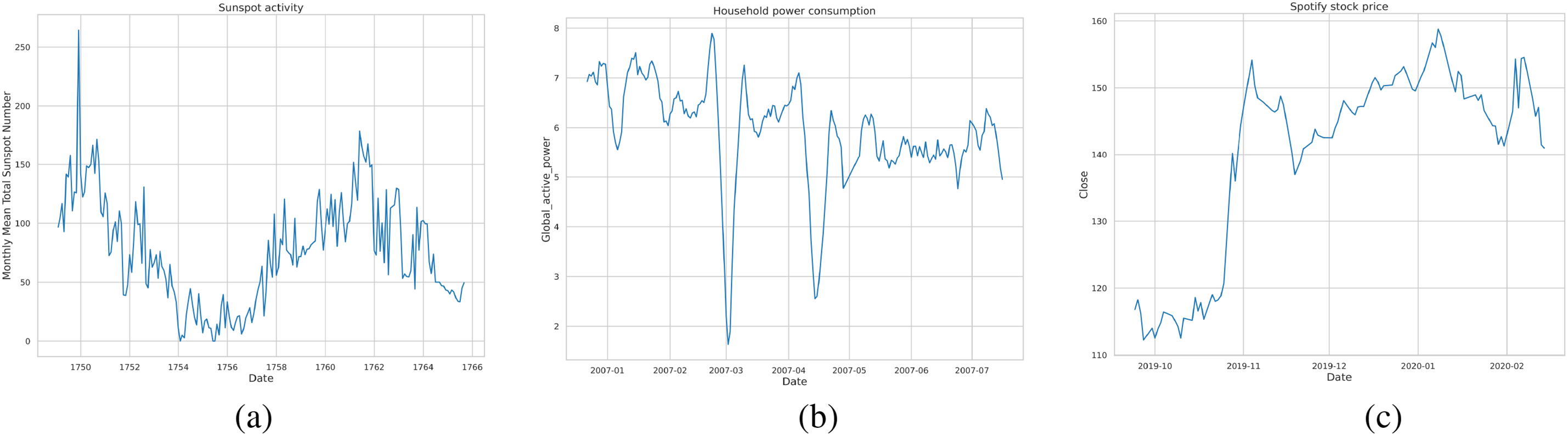
Figure 1: Sample data from the tree datasets used in this study: (a) Monthly mean total sunspot number, (b) Household power consumption, and (c) Spotify stock prices
Household power consumption [21], the dataset covers residential electricity consumption from December 2006 to November 2010. The data contains measurements of electricity consumption per household at a frequency of once per minute, which allows the model to identify short-term and long-term patterns. For the analysis, the variable “Global_active_power” was used, which reflects the total active electricity consumption in kilowatts.
Monthly mean total sunspot number [22], the dataset contains information on the monthly average number of sunspots for the period from 1749 to 2013. This long-term time series covers more than 260 years of observations, which allows the model to be trained on data with well-defined long-term cycles, including the well-known 11-year solar activity cycles.
Spotify stock price [23], the dataset represents the daily closing prices of Spotify shares over the past five years, obtained from Yahoo Finance. This time series is characterized by high volatility and random fluctuations, which are typical for financial markets. Using this dataset allows us to test the model’s robustness to noise and its ability to predict financial time series.
Prior to training the model, thorough data preprocessing was performed for each set to ensure the quality and relevance of the input data.
First, we analyzed for data gaps. The electricity consumption dataset revealed gaps that occurred due to technical failures or missing observations. These gaps were filled using linear interpolation, which allowed us to maintain the continuity of the time series. In the case of sunspot data, the gaps were minimal and were filled with the average values of neighboring points. For Spotify share price data, gaps occurred due to non-working days on the stock exchange. These gaps were filled using the last known value forward-fill method, which is acceptable for financial time series.
Second, outliers were identified and processed. Statistical methods, such as interquartile range (IQR) analysis, were used to identify outliers that differed significantly from other observations. Outliers could distort the modeling results, so they were replaced with median values or smoothed using a moving average. This helped reduce the impact of extreme values on model training.
The next step was to normalize and scale the data. Since different variables could have different scales and units of measurement, it was important to bring them to a single range. To do this, we used the min-max scaling method, which converts the data to the range [0, 1]. The formula for min-max scaling is shown in Eq. (1):
This made it possible to improve the stability of model training and prevent a situation where variables with higher values dominate over others.
Next, we generated training samples. To do this, we used the windowing method, which converts a time series into a set of input and output sequences. A fixed window of previous values of size window_size was chosen as input and a corresponding number of subsequent values of size predict_size as target values for prediction. This allowed the model to learn to predict not only a single future value but also a sequence of future values.
To solve the problem of time series forecasting, we propose the FractalNet-LSTM model. The general structure of FractalNet-LSTM is shown in Fig. 2. In particular, we implement a fractal convolutional encoder that extracts multiscale features from input sequences by capturing local patterns at different levels of abstraction. Similar to recent works exploring fractional-order neural networks [24], this design emphasizes feature extraction at various scales. Next, we develop a recurrent decoder based on LSTM layers to model temporal dependencies and enhance long-term dependencies between sequences. Finally, the output layer of FractalNet-LSTM is built using a fully connected layer that generates the final prediction. The technical details of each component of FractalNet-LSTM are described in detail in the following sections.
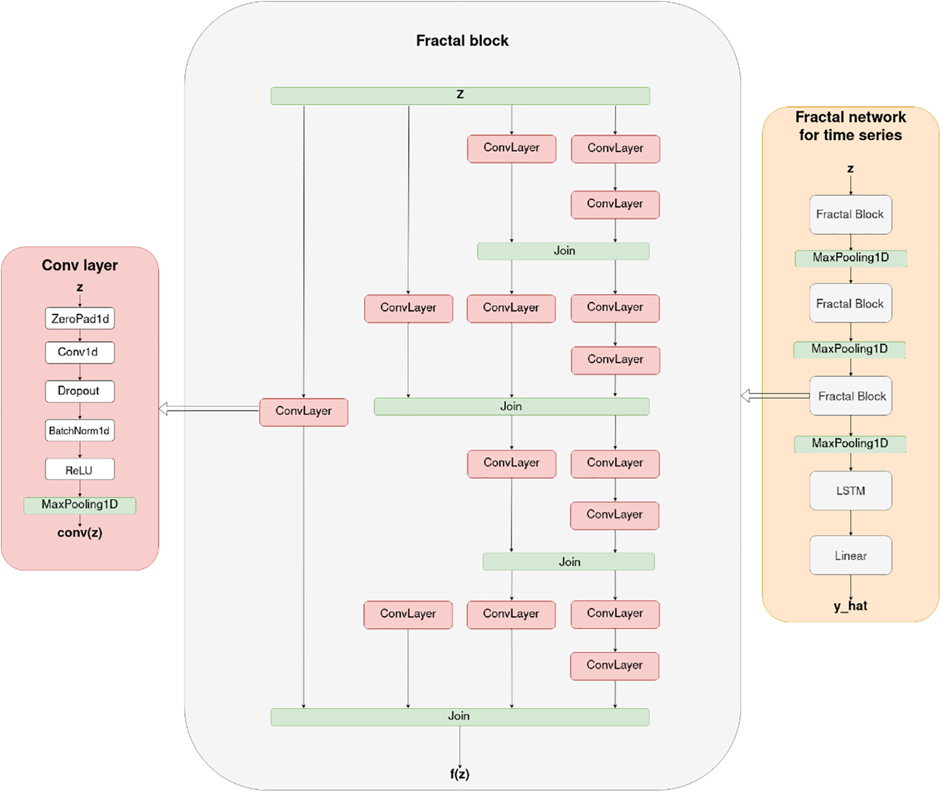
Figure 2: The general structure of the proposed FractalNet-LSTM model
The main components of the architecture include:
1. Fractal convolutional blocks: Each block consists of multiple parallel paths containing sequences of one-dimensional convolutional layers (Conv1D), batch normalization layers (BatchNormalization), regularization layers (Dropout), and ReLU activation functions. Convolutional layers extract local features from the input data, and parallel branches allow the model to simultaneously process information at different scales;
2. Combining outputs: The outputs of parallel branches are combined using an averaging or concatenation mechanism. This allows you to integrate information from different levels of abstraction and improves the model’s ability to generalize;
3. LSTM layer: After the fractal blocks, an LSTM layer is used to process the sequence of extracted features. The LSTM can store information about previous states and take into account long-term dependencies, which is critical for time series;
4. Output fully connected layer: The final layer of the model is the Linear layer, which converts the LSTM output into predicted values.
The use of fractal convolutional blocks in combination with LSTM allows the model to efficiently extract both local and global features from the data, which improves the prediction accuracy.
The design of the fractal convolutional blocks in FractalNet-LSTM is founded on the principles of self-similarity and multi-scale feature extraction inherent to fractal geometry. Each fractal block comprises multiple parallel convolutional paths with varying kernel sizes and depths, enabling the model to capture patterns at different temporal scales. To adapt the fractal blocks for new datasets, one can adjust the number of columns, the initial number of channels, and the dropout probabilities based on the specific characteristics of the dataset. For instance, datasets with more complex or longer-term dependencies may benefit from increased depth or additional parallel paths within the fractal blocks. Furthermore, the kernel sizes can be modified to better align with the inherent periodicities or trend lengths in the data. By tuning these hyperparameters, the fractal convolutional blocks can be effectively redesigned to suit the unique requirements of various time series datasets, thereby enhancing the model’s adaptability and performance across diverse forecasting tasks.
For training the proposed FractalNet-LSTM and baseline models, we utilized the Adam optimizer with a learning rate of 1e − 3 and a weight decay of 1e − 4 across all experiments. To enhance training efficiency and prevent overfitting, we implemented the “ReduceLROnPlateau” scheduler, which reduces the learning rate by a factor of 0.5 if the validation loss does not improve for 20 consecutive epochs. Additionally, we employed “EarlyStopping” with a patience of 50 epochs to terminate training early if no improvement in validation loss was observed, thereby saving computational resources and avoiding overfitting.
The loss function used during training was the Huber loss, which combines the robustness of MAE with the sensitivity of MSE to larger errors, making it suitable for handling outliers in the data. For evaluation during the testing phase, we employed the following metrics: MAE, MAPE, RMSE, R2, and Huber loss. These metrics were consistently applied across all datasets to ensure a fair and comprehensive comparison of model performance.
Each model was trained separately on the respective datasets (electricity consumption, sunspot activity, and Spotify stock prices) using the same training parameters to maintain consistency and fairness in the experimental results. Detailed initialization parameters for each model run, including window size, batch size, and other hyperparameters, are provided in config files inside the repository.
To illustrate each step of the predictive model, suppose we have a simplified one-dimensional time series with daily measurements
1. Input Window. We select days 1, 2, and 3 as inputs, labeled
2. Fractal Convolution Blocks. Parallel Convolution Paths: Each path applies a different Conv1D kernel (for example, sizes 1, 2, and 3) to capture local patterns at multiple scales. Batch Normalization and ReLU: After each convolution, batch normalization stabilizes feature distributions, and the ReLU activation adds nonlinearity. Dropout (Regularization): Dropout layers reduce overfitting by randomly ‘dropping’ a fraction of neurons during training. Output Merging: Outputs from each parallel path are combined (e.g., concatenated) into a single feature matrix.
3. LSTM Layer. Sequential Processing: The merged features, now shaped as a short sequence, enter the LSTM. Memory Cell and Gates: The LSTM retains information about past states, learning longer-term dependencies that may span beyond the 3-day window.
4. Output Fully Connected Layer. Dense Layer: A linear (fully connected) layer processes the final hidden state of the LSTM to generate the model’s prediction. Predicted Values: In this toy example, the layer outputs two values,
By repeating the above process on many overlapping windows from the training dataset, FractalNet-LSTM learns a comprehensive mapping between past observations
To quantify the accuracy and efficiency of the proposed models, several metrics were used to evaluate various aspects of performance in time series forecasting.
MAE is one of the main indicators of model accuracy. It is calculated as the average of the absolute differences between the actual values and the predicted model values. The Eq. (2) for MAE is as follows:
where
The MAPE expresses the error as a percentage of the actual value, which allows you to evaluate the accuracy of the forecast regardless of the scale of the data. The Eq. (3) for MAPE:
RMSE gives more weight to larger deviations because the error is squared before being averaged. This makes RMSE sensitive to large errors, which is important in the context of forecasting. The Eq. (4) for RMSE:
The Huber loss function combines the properties of MAE and MSE to provide robustness to outliers. It uses a quadratic function for small errors and a linear function for large errors, reducing the impact of anomalous values. The Eqs. (5) and (6) is defined as:
where δ is the threshold that determines the transition between the quadratic and linear parts of the function.
The coefficient of determination (
where
The use of these metrics provides a comprehensive assessment of the models, allowing for analysis of their accuracy, robustness to outliers, and ability to explain variations in the data. Low values of MAE, MAPE, and RMSE indicate high model accuracy, while a high R2 determination coefficient confirms that the model models the relationship between input and output data well.
During the experiments, these metrics were used to compare the performance of the proposed FractalNet-LSTM model with the baseline models. This approach allowed us to objectively evaluate the advantages and disadvantages of each model and draw conclusions about their suitability for different types of time series.
3 Baseline Methods and Results
To objectively evaluate the effectiveness of the proposed FractalNet-LSTM model, we compared it with other well-known neural network architectures that are widely used in time series forecasting tasks. In particular, the following basic models were selected: standard LSTM, bidirectional LSTM (BiLSTM), NAR, and the combined CNN-LSTM model.
The LSTM model is a classical recurrent neural network specifically designed to model long-term dependencies in sequential data. Through the use of memory cells and gate mechanisms (input, forgetting, and output), LSTM efficiently stores and transmits information over long periods of time, preventing the problem of gradient vanishing. In the context of time series forecasting, LSTM allows the model to take into account both short-term and long-term patterns, which is critical for accurately predicting future values.
Bi-directional LSTM extends the standard LSTM architecture by allowing the model to process a data sequence in both the forward (past to future) and backward (future to past) directions. This provides a more complete capture of context, as the model takes into account information on both sides of each element in the sequence. In some tasks, this can improve the quality of forecasting, especially when future states affect current ones. However, in time series forecasting tasks, the use of BiLSTM has limitations, since the model does not have access to future data when predicting future values. Nevertheless, the inclusion of BiLSTM in the comparison allows us to evaluate the potential advantages of this architecture in the context of time series processing.
The NAR model was included in our comparative analysis due to its robust capability to capture complex temporal dependencies in time series forecasting. NAR is a type of feedforward neural network that models the current output as a nonlinear function of its past outputs, enabling it to effectively recognize and represent intricate patterns and interactions within the data. Unlike standard autoregressive models, NAR can handle nonlinear relationships, which enhances its ability to model sophisticated dynamics inherent in various time-dependent datasets. By incorporating historical information through the inclusion of lagged outputs as input features, NAR allows the model to anticipate future values based solely on its own previous states. This autoregressive dependency facilitates more accurate and reliable predictions, particularly in scenarios where the underlying processes exhibit nonlinear behavior. Including NAR in our evaluation provides a comprehensive benchmark against which the performance of the proposed FractalNet-LSTM model can be assessed, highlighting the strengths and potential improvements of our approach in handling nonlinear temporal dependencies in forecasting tasks.
The combined CNN-LSTM model combines the capabilities of CNNs and LSTMs to process time series. In this architecture, CNN is used to extract local features from the input data. Convolutional CNN layers effectively detect local patterns and relationships in sequences, which can be especially useful when working with data that has local dependencies or repeated structures. After that, the extracted features are passed to the LSTM layer, which models long-term dependencies and takes into account the sequence of data over time. This combination allows the model to simultaneously take into account both local and global patterns, which can improve the accuracy of forecasting.
All basic models were implemented using the same principles and tools as the proposed FractalNet-LSTM model. The following conditions were met to ensure a fair comparison:
• Data sets: The models were trained and tested on the same datasets of electricity consumption, sunspot activity, and Spotify stock prices;
• Pre-processing: The same preprocessing techniques were applied to the data, including gap filling, normalization, and training set generation;
• Data split: The same data split was used for all datasets and models: 70% for training, 15% for validation, and 15% for testing.
• Training conditions: We used the same loss functions (MSE or Huber Loss), optimizers (Adam), and training stopping criteria (early stopping based on validation error);
• Evaluation metrics: The performance of the models was evaluated using the same metrics: MAE, MAPE, RMSE, R2, and Huber’s loss function.
The combined CNN-LSTM model combines the capabilities of CNNs and LSTMs to process time series. In this architecture, CNN is used to extract local features from the input data. Convolutional CNN layers effectively detect local patterns and relationships in sequences, which can be especially useful when working with data that has local dependencies or repeated structures. After that, the extracted features are passed to the LSTM layer, which models long-term dependencies and takes into account the sequence of data over time. This combination allows the model to simultaneously take into account both local and global patterns, which can improve the accuracy of forecasting.
Table 1 shows the results of the FractalNet-LSTM, LSTM, BiLSTM, NAR, and CNN-LSTM models for different forecast horizons on sunspot activity data. Also, a comparison of models by MAE and RMSE metrics can be seen in Fig. 3.

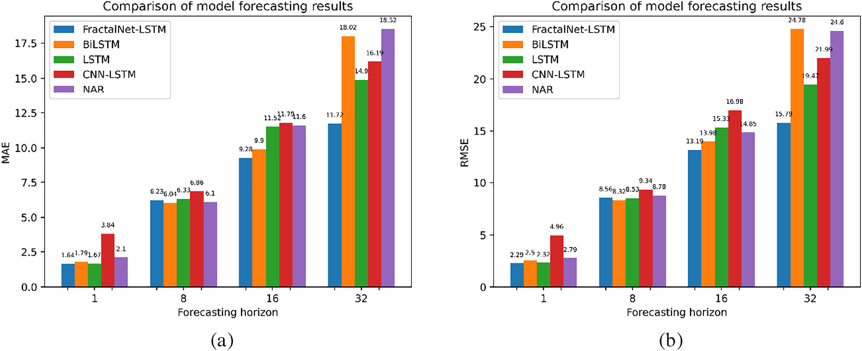
Figure 3: Comparison of model forecasting results on sunspot activity dataset by: (a) MAE; (b) RMSE metrics
When forecasting a single point, the BiLSTM model performed the best with the lowest MAE (1.64) and highest R2 (0.9960), indicating its high accuracy in short-term forecasting. FractalNet-LSTM and LSTM also demonstrate high accuracy with a slight lag.
At a forecast horizon of 8 points, FractalNet-LSTM outperforms the other models, achieving the lowest MAE (6.23) and MAPE (15.8%), as well as the highest R2 (0.9205). This indicates the model’s ability to effectively model medium-term patterns in the data.
For the 16-point horizon, BiLSTM and FractalNet-LSTM show similar results, with BiLSTM slightly ahead in terms of MAE (9.90 vs. 9.28). However, the R2 for both models decreases, indicating the difficulty of long-term forecasting.
At a long horizon of 32 points, FractalNet-LSTM again performs best with MAE (11.72) and R2 (0.5986), outperforming the other models. This indicates that the fractal architecture helps the model to better detect long-term dependencies in the data.
3.2.2 Household Power Consumption
Table 2 shows the results in household power consumption data. Comparison by MAE and RMSE metrics can be seen in Fig. 4.

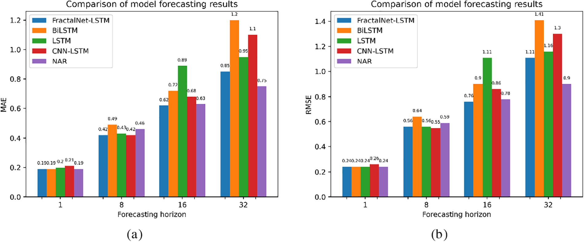
Figure 4: Comparison of model forecasting results on household power consumption dataset by: (a) MAE; (b) RMSE metrics
At a short horizon (1 point), BiLSTM, NAR, and FractalNet-LSTM performed best with MAE (0.19) and low MAPE. This indicates their ability to accurately predict short-term changes in electricity consumption.
At the 8-point horizon, FractalNet-LSTM and CNN-LSTM performed similarly with MAE (0.42). However, the CNN-LSTM has a slightly higher R2 (0.2000), indicating a better fit of the model to the data.
When forecasting 16 points, FractalNet-LSTM retains the lowest MAE (0.62) and MAPE (16.0%), although R2 becomes negative, indicating a decrease in model accuracy compared to the simple average.
At a long horizon of 32 points, NAR demonstrates the best results in terms of MAE (0.75), FractalNet-LSTM is second place with MAE (0.85), but all models show a decrease in accuracy, which indicates the complexity of long-term electricity consumption forecasting.
Similar to the previous sections, Table 3 shows the results in Spotify stock price data. A comparison by MAE and RMSE metrics can be seen in Fig. 5.
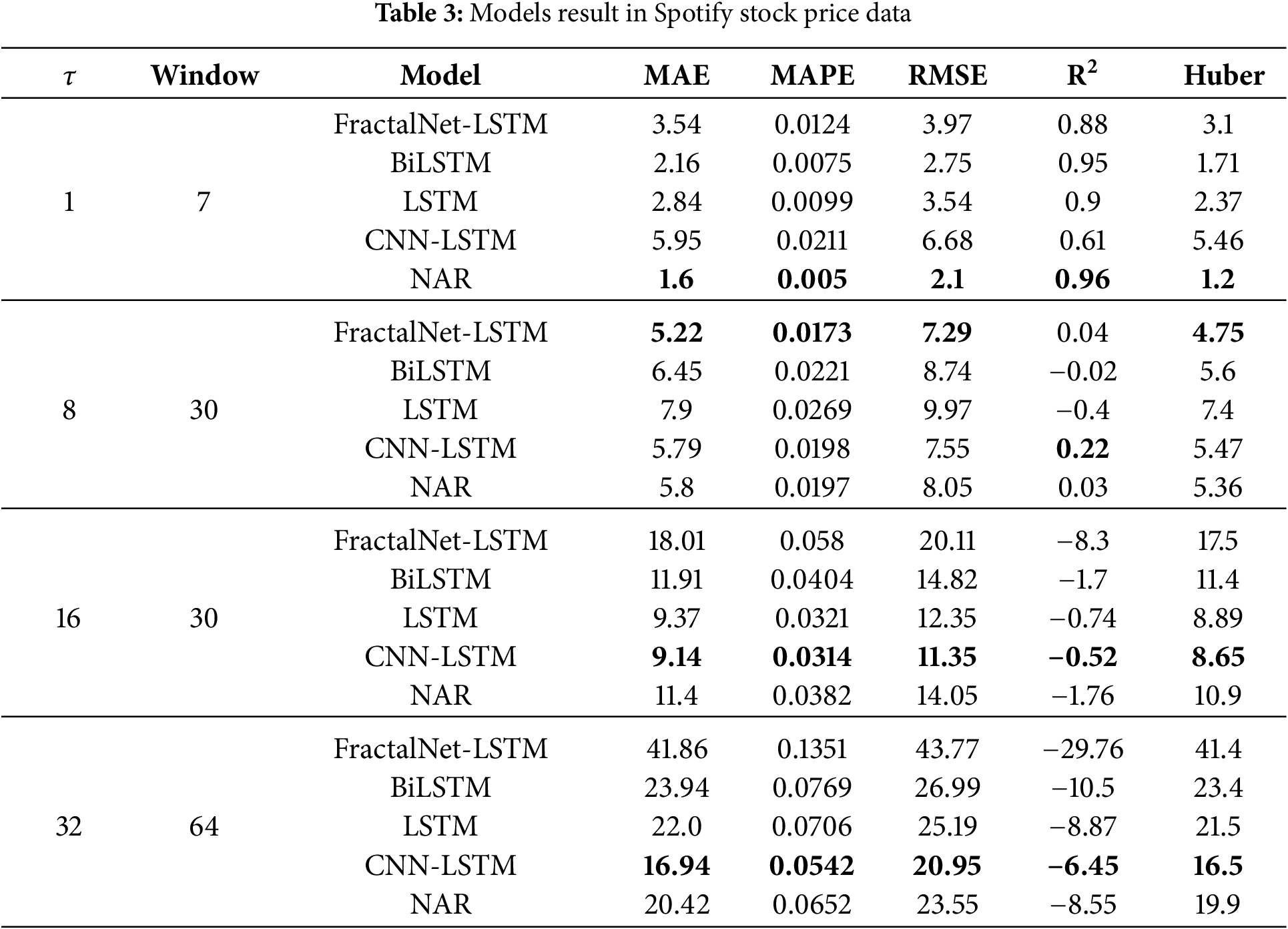
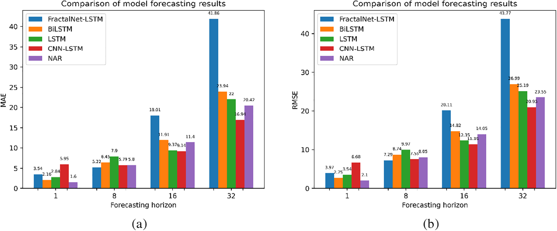
Figure 5: Comparison of model forecasting results on Spotify stock price dataset by: (a) MAE; (b) RMSE metrics
On the short horizon (1 point), NAR shows the best results with MAE (1.6) and R2 (0.96). FractalNet-LSTM lags behind BiLSTM and LSTM, which may indicate that for financial data with high volatility, the fractal architecture is less effective in short-term forecasting.
At the 8-point horizon, FractalNet-LSTM demonstrates the lowest MAE (5.22) and MAPE (1.73%), but its R2 is lower than that of CNN-LSTM (0.0400 vs. 0.2200). This indicates that although FractalNet-LSTM has a better average error, its fit to the data overall may be worse.
For the 16 and 32 point horizons, CNN-LSTM performs the best in terms of MAE and RMSE among all models, although all models exhibit negative R2 values, indicating a significant decrease in accuracy for long-term forecasting.
FractalNet-LSTM is significantly inferior to the other models at long horizons, which may be due to the complexity of financial data and high volatility, which is difficult to model even with sophisticated architectures.
In this study, we proposed the FractalNet-LSTM model, which combines fractal convolutional blocks with recurrent LSTM layers to improve the accuracy of time series forecasting. The results show that the proposed model outperforms traditional approaches at medium forecasting horizons and demonstrates high accuracy for data with long-term and cyclic dependencies.
Analysis of the results. On the sunspot activity and household electricity consumption datasets, FractalNet-LSTM performed particularly well at medium forecast horizons (8 and 16 points). This can be explained by the ability of the fractal architecture to effectively detect complex patterns and multi-level dependencies in the data. The fractal convolutional units allow the model to extract features at different scales, which is critical for time series with long cycles, such as 11-year solar activity cycles.
Compared to baseline models such as standard LSTM and BiLSTM, FractalNet-LSTM demonstrates competitive or even superior performance at medium and long horizons. This suggests that the addition of fractal structure improves the model’s ability to detect global patterns and model long-term dependencies.
However, at short forecast horizons (1 point), BiLSTM often outperforms FractalNet-LSTM. This may be due to the fact that BiLSTM takes into account information from both the past and the future, although in tasks of predicting future values, access to future data is limited. Nevertheless, FractalNet-LSTM still demonstrates high accuracy on short horizons, which emphasizes its versatility.
Limitations and challenges. Although the FractalNet-LSTM approach has proven effective in various scenarios, it also faces potential difficulties that include high computational complexity arising from the parallel “branches” within the fractal blocks, the risk of overfitting when the available dataset is limited due to the depth and complexity of the architecture, and difficulties in tuning the large number of hyperparameters typical for fractal and LSTM-based models. Additionally, the model exhibits sensitivity to highly volatile financial time series such as the Spotify dataset, where the presence of noise can overshadow the benefits of fractal structures, particularly over long forecasting horizons. While fractal convolutional blocks help capture multi-scale features, the LSTM’s memory mechanisms may not suffice to retain or generalize information under these conditions, often leading to negative R2 values and decreased accuracy. These issues reflect the inherent complexity of long-term forecasting and emphasize the need for extensive amounts of data and additional strategies (e.g., more robust regularization or specialized volatility modeling) when dealing with data dominated by randomness.
Comparison with previous studies. The results of our study are consistent with previous works that indicate the effectiveness of using fractal neural networks to model complex nonlinear dependencies [15,16]. Previous studies have shown that fractal networks can improve the generalization ability of models and increase their resistance to noise [17]. Our results confirm these findings and demonstrate that the integration of fractal properties into neural networks is a promising direction for improving time series forecasting.
Compared to baseline models such as standard LSTM and BiLSTM, FractalNet-LSTM demonstrates competitive or even superior performance at medium and long horizons. This observation aligns with the findings of other reviews on the strengths and limitations of LSTM-based forecasting [25].
Practical implications. The results have important practical implications. The FractalNet-LSTM model can be used to improve forecasting accuracy in industries where time series have long-term and cyclical dependencies, such as energy and meteorology. This can contribute to more informed decision-making and resource optimization.
Directions for future research. Further research could be aimed at adapting FractalNet-LSTM to work with highly volatile data, including financial data. A possible approach is to integrate noise processing methods or use hybrid architectures that combine fractal networks with other noise-resistant models.
In addition, it is worth exploring the possibility of automatically adjusting the depth and structure of fractal blocks depending on the characteristics of the data. This will improve the adaptability of the model and its versatility for different types of time series.
Overall, the study shows that integrating fractal properties into neural network architecture improves the accuracy of time series forecasting. FractalNet-LSTM demonstrates advantages at medium forecasting horizons and for data with long-term dependencies. This opens up new opportunities for developing more accurate and reliable forecasting systems that can be applied in various industries.
Furthermore, the outcomes of this research hold practical relevance for a wide range of real-world applications, such as forecasting energy consumption to optimize power grid operations, improving meteorological predictions for resource management, and supporting long-term strategic planning in diverse industrial sectors. For high-volatility financial time series, additional noise suppression or specialized filtering methods may be necessary to achieve robust performance. Future work could explore adaptive fractal networks, hybrid solutions that incorporate attention mechanisms, and pre-trained models to further enhance the flexibility and resilience of FractalNet-LSTM across different data domains.
Acknowledgement: The authors would like to thank editors and reviewers for their valuable work.
Funding Statement: This research received no external funding.
Author Contributions: The authors confirm contribution to the paper as follows: study conception and design: Nataliya Shakhovska and Volodymyr Shymanskyi; data collection: Maksym Prymachenko; analysis and interpretation of results: Nataliya Shakhovska, Volodymyr Shymanskyi and Maksym Prymachenko; draft manuscript preparation: Volodymyr Shymanskyi and Maksym Prymachenko. All authors reviewed the results and approved the final version of the manuscript.
Availability of Data and Materials: The data that support the findings of this study are openly available in: “Electric Power Consumption Data Set” at https://www.kaggle.com/datasets/uciml/electric-power-consumption-data-set (accessed on 20 October 2024); “Monthly Mean Total Sunspot Number” at https://www.kaggle.com/datasets/robervalt/sunspots (accessed on 20 October 2024); “Spotify Technology S.A. (SPOT) Stock Price Data” at https://finance.yahoo.com/quote/SPOT (accessed on 20 October 2024). The code, model configurations, and architectural definitions necessary to reproduce the experiments presented in this study are publicly available in the GitHub repository at https://github.com/MaksymPrymachenko/FractalNet_TimeSeries (accessed on 07 February 2025). This repository includes all configuration files for the models, architectures, and the complete codebase required to replicate the experimental setup and results. Comprehensive instructions are provided to facilitate the seamless reproduction of our experiments.
Ethics Approval: Not applicable.
Conflicts of Interest: The authors declare no conflicts of interest to report regarding the present study.
References
1. Hyndman RJ, Athanasopoulos G. Forecasting: principles and practice. 2nd ed. Australia: OTexts; 2018. [Google Scholar]
2. Box GEP, Jenkins GM, Reinsel GC, Ljung GM. Time series analysis: forecasting and control. 5th ed. Hoboken, NJ, USA: Wiley; 2016. [Google Scholar]
3. Chatfield C. The analysis of time series: an introduction. 6th ed. Boca Raton, FL, USA: Chapman & Hall/CRC; 2016. [Google Scholar]
4. Hamilton JD. Time series analysis. Princeton, NJ, USA: Princeton University Press; 1994. [Google Scholar]
5. Kolemen E, Egrioglu E, Bas E, Turkmen M. A new deep recurrent hybrid artificial neural network of gated recurrent units and simple seasonal exponential smoothing. Granul Comput. 2023;9(1):7. doi:10.1007/s41066-023-00444-4. [Google Scholar] [CrossRef]
6. Kirichenko L, Koval Y, Yakovlev S, Chumachenko D. Anomaly detection in fractal time series with LSTM autoencoders. Mathematics. 2024;12(19):3079. doi:10.3390/math12193079. [Google Scholar] [CrossRef]
7. Goodfellow I, Courville A, Bengio Y. Deep learning. in adaptive computation and machine learning. Cambridge, MA, USA: The MIT Press; 2016. [Google Scholar]
8. LeCun Y, Bengio Y, Hinton G. Deep learning. Nature. 2015;521(7553):436–44. doi:10.1038/nature14539. [Google Scholar] [PubMed] [CrossRef]
9. Hochreiter S, Schmidhuber J. Long short-term memory. Neural Comput. 1997;9(8):1735–80. doi:10.1162/neco.1997.9.8.1735. [Google Scholar] [PubMed] [CrossRef]
10. Cho K, Van Merrienboer B, Gulcehre C, Bahdanau D, Bougares F, Schwenk H, et al. Learning phrase representations using RNN encoder-decoder for statistical machine translation. arXiv:1406.1078. 2014. [Google Scholar]
11. Kong Y, Wang Z, Nie Y, Zhou T, Zohren S, Liang Y, et al. Unlocking the power of LSTM for long term time series forecasting. arXiv:2408.10006. 2024. [Google Scholar]
12. Shakhovska N, Medykovskyi M, Gurbych O, Mamchur M, Melnyk M. Enhancing solar energy production forecasting using advanced machine learning and deep learning techniques: a comprehensive study on the impact of meteorological data. Comput Mater Contin. 2024;81(2):3147–63. doi:10.32604/cmc.2024.056542. [Google Scholar] [CrossRef]
13. Srivastava N, Hinton G, Krizhevsky A, Sutskever I, Salakhutdinov R. Dropout: a simple way to prevent neural networks from overfitting. J Mach Learn Res. 2014;15(56):1929–58. [Google Scholar]
14. Kaminsky R, Mochurad L, Shakhovska N, Melnykova N. Calculation of the exact value of the fractal dimension in the time series for the box-counting method. In: 2019 9th International Conference on Advanced Computer Information Technologies (ACIT); 2019 Jun 5–7; Ceske Budejovice, Czech Republic: IEEE. Vol. 2019, p. 248–51. doi:10.1109/ACITT.2019.8780028. [Google Scholar] [CrossRef]
15. Kirkby MJ. The fractal geometry of nature. Benoit B. Mandelbrot. W. H. Freeman and co., San Francisco, 1982. No. of pages: 460. Price: £22.75 (hardback). Earth Surf Processes Landf. 1983;8(4):406. doi:10.1002/esp.3290080415. [Google Scholar] [CrossRef]
16. Larsson G, Maire M, Shakhnarovich G. FractalNet: ultra-deep neural networks without residuals. arXiv:1605.07648. 2016. [Google Scholar]
17. Baicoianu A, Gavrilă CG, Pacurar CM, Pacurar VD. Fractal interpolation in the context of prediction accuracy optimization. arXiv:2403.00403. 2024. [Google Scholar]
18. Shymanskyi V, Ratinskiy O, Shakhovska N. Fractal neural network approach for analyzing satellite images. Appl Artif Intell. 2025;39(1):2440839. doi:10.1080/08839514.2024.2440839. [Google Scholar] [CrossRef]
19. Zhang G, Eddy Patuwo B, Hu MY. Forecasting with artificial neural networks. Int J Forecast. 1998;14(1):35–62. doi:10.1016/S0169-2070(97)00044-7. [Google Scholar] [CrossRef]
20. Casolaro A, Capone V, Iannuzzo G, Camastra F. Deep learning for time series forecasting: advances and open problems. Information. 2023;14(11):598. doi:10.3390/info14110598. [Google Scholar] [CrossRef]
21. UCI Machine Learning Repository. Household electric power consumption time series analysis-regression/clustering [Internet]. 2024 [cited 2024 Oct 20]. Available from: https://www.kaggle.com/datasets/uciml/electric-power-consumption-data-set. [Google Scholar]
22. Robert V. Monthly mean total sunspot number [Internet]. 2024 [cited 2024 Oct 20]. Available from: https://www.kaggle.com/datasets/robervalt/sunspots. [Google Scholar]
23. Yahoo Finance. Spotify technology S.A. (SPOT) stock price data [Internet]. 2024 [cited 2024 Oct 20]. Available from: https://finance.yahoo.com/quote/SPOT. [Google Scholar]
24. Zhao C, Ye J, Zhu Z, Huang Y. FLRNN-FGA: fractional-order lipschitz recurrent neural network with frequency-domain gated attention mechanism for time series forecasting. Fractal Fract. 2024;8(7):433. doi:10.3390/fractalfract8070433. [Google Scholar] [CrossRef]
25. Kader NIA, Yusof UK, Khalid MNA, Husain NRN. A review of long short-term memory approach for time series analysis and forecasting. In: Proceedings of the 2nd International Conference on Emerging Technologies and Intelligent Systems; 2023. Vol. 573. p. 12–21. [Google Scholar]
Cite This Article
 Copyright © 2025 The Author(s). Published by Tech Science Press.
This work is licensed under a Creative Commons Attribution 4.0 International License , which permits unrestricted use, distribution, and reproduction in any medium, provided the original work is properly cited.
 Downloads
 Citation Tools