TMRE: Novel Algorithm for Computing Daily Reference Evapotranspiration Using Transformer-Based Models

1  Introduction

Evapotranspiration is the mechanism through which water evaporates from the surface of the soil, groundwater, and land-based water reservoirs, as well as from the surface of plants as a result of transpiration and evaporation. This parameter varies for each crop; however, it is easily computed by multiplying the evapotranspiration of a reference crop and the crop constant for that crop. Reference evapotranspiration (ETo) is measured from the reference crop, such as grass [1]. As a result, precise ETo calculations are essential for improving water resource management and setting more accurate irrigation plans [2]. Furthermore, it has much influence in arid and semi-arid countries, where high crop water demands and low precipitation limit crop growth and agricultural output, as water access is the most pressing issue in these areas. It is important that semi-arid zones cover 15.2% of the planet’s land surface and are the majority of the surface area1. Hence, accurate ETo forecasting is critical for meeting the water needs of these arid lands to meet their needs.

FAO-56 Penman-Monteith (PM) (FAO stands for United Nations Food and Agriculture Organization) is the most extensively used strategy for calculating ETo and testing other ETo methods [3]. FAO-56 PM calculates ETo using semi-empirical as well as semi-physical methods; however, it requires a handful of input parameters such as average, minimum and maximum temperature, average wind speed, relative humidity (RH), and hours of sunlight (n). Building and maintaining equipment that can measure all necessary factors, such as atmospheric temperature, humidity level, wind speed, and solar irradiance, is prohibitively expensive. It is required to investigate a less complex model to estimate future ETo values with an outstanding level of accuracy while using minimal meteorological features. In addition to the FAO method, there are other methods that are also expensive [1].

With the recent advances in artificial intelligence concepts and computing capacity, the challenge of computing ETo from meteorological data has been viewed as a time series regression/forecasting problem that can be addressed by certain deep learning (DL) and machine learning (ML) models [4,5]. The aim was achieved by using various ML algorithms. For example, Youssef et al. [6] employed three ML models, namely SVM (Support Vector Machine), M5P and RF (Random Forest) with some empirical models for monthly ETo prediction in two regions of India using monthly climate data from 2009 to 2016 (8 years). The findings showed that the SVM model outperformed the other ML and empirical models at every station. Another study by Saggi et al. [7] on meteorological data from several places in India and Spain discovered that machine learning models outperformed traditional methods of estimating ETo. Kumar [8] developed multiple ML algorithms using meteorological data from January 1985 to December 2010, with the RF and gradient boosting regression (GBR) doing well.

Artificial neural networks (ANN) are popular ML models and deep learning (DL) that perform well compared to traditional machine learning models for time series prediction. For monthly ETo in India and Algeria, Tikhamarine et al. [9] utilized an ANN with five distinct optimizers, while the results demonstrated the efficiency of the grey-wolf optimizer (GWO). Chen et al. [10] employed a deep neural network (DNN), a Long short-term memory (LSTM) and a temporal convolution neural network (TCNN) model to estimate ETo in China’s Northeast Plain using meteorological data, with TCNN being better than standard ML models. Kahn et al. [11] also explored the estimation of evapotranspiration (ET) for saline soils, by introducing an IoT (Internet of Things)-enabled architecture that used crop field contexts, such as soil and irrigation water salinity, and temperature, to predict monthly ET for saline soils using Long Short-Term Memory (LSTM) and ensemble LSTM models.

Many studies used the Ensemble learning technique, combining predictions from multiple models to provide an improved and effective final prediction. Salahuddin et al. [12] employed ensemble learning to conduct sensitivity analysis, applying ML techniques such as a single decision tree, a tree boost, and a decision tree forest. Sharma et al. [13] presented a method named DeepEvap. It is a deep reinforcement learning-based method that outperforms the prediction results of four different deep neural network-based models CNN-LSTM, Convolutions with LSTM, CNN with support vector regression, and CNN (Convolutional Neural Network) with GBR for ETo estimation using meteorological dataset.

Although machine learning (ML) and deep learning (DL) models have shown good performance across various datasets, recently developed transformer models have also been proven to be state of art. Transformers that were crafted initially for natural language processing (NLP) problems [14], since been modified for use in computer vision applications [15,16] and have now been enhanced and utilized for time series forecasting as well [17,18]. Bellido-Jiménez et al. [19] also computed daily ETo from an Andalusian meteorological dataset using two networks: CNN-transformers and LSTM-transformers. CNN-transformers employed CNN in their feed-forward layers, whereas LSTM-transformers utilized LSTM.

After the advent of transformers in time series, several models were built based on its architecture. For instance, the informer replaced the self-attention mechanism with sparse attention [20]. Then, there is an architecture called Autoformer [21] in which auto-correlation was used instead of self-attention. Then comes FEDformer [22] which claims to be more efficient than all discussed previously. This paper uses four different transformer-based models: transformer with self-attention, informer with prob-sparse attention, Autoformer with autocorrelation mechanism, and FEDformer to model daily ETo.

Existing approaches to ETo forecasting have achieved only moderate success, as traditional machine learning and deep learning models struggle to fully capture the complex multivariate and seasonal dependencies inherent in ETo data. While transformer-based architectures have shown promise in time-series forecasting, their potential remains underexplored in ETo, with limited comparative analysis of advanced variants like Informer, Autoformer, and FEDformer. Additionally, many existing methods employ fixed or arbitrary window sizes, neglecting the importance of optimizing window selection based on seasonal trends and variations, which is critical for improving predictive performance. This gap in leveraging advanced models and optimized window-sizing strategies motivates the need for a more systematic and effective approach to ETo forecasting. A workflow of the proposed research is given in Fig. 1. The primary contributions of this study are:

Figure 1: Workflow diagram of the proposed research

•   The predictability of the time-series problem was increased by capturing distinct long-range dependencies between inputs and outputs in long-sequence time-series tasks using transformer-based models.

•   Various transformer-based methods were investigated to analyse forecast efficiency based on the dataset’s features.

The following sections of this paper are arranged as follows. Section 2 provides a discussion of the dataset and technique used in this analysis. In Section 3, experiments are discussed. The results and discussions about the experiments are presented in Section 4. Section 5 concludes the paper.

2  Materials and Methods

This section discusses the dataset with its preprocessing steps and methods for time series forecasting.

2.1 Dataset

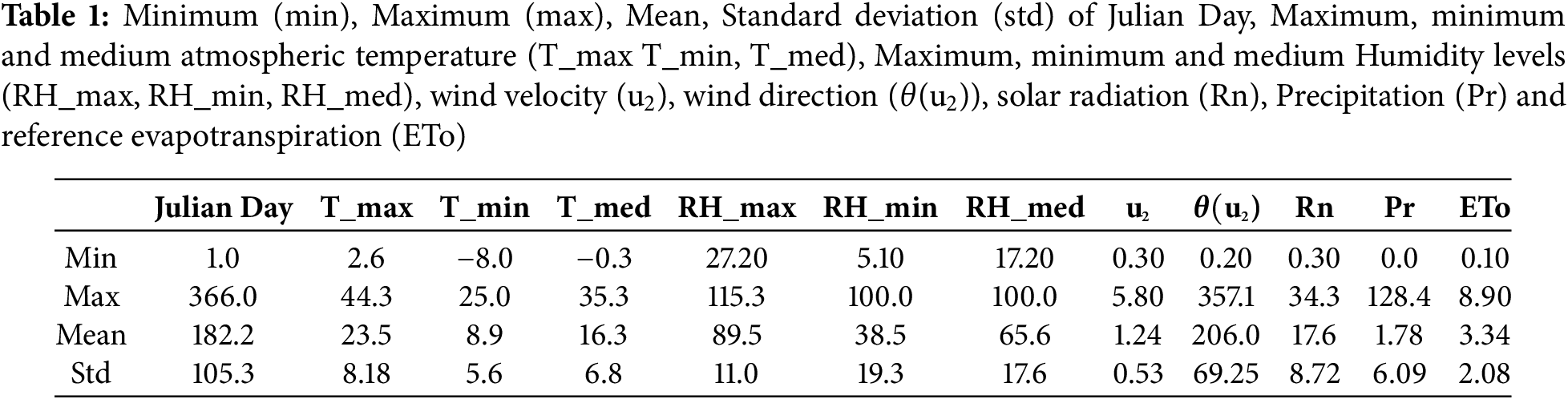
Aroche is located in Andalusia, southwest of Europe. Its latitude and longitude are 37.9437° N and 6.9545° W, respectively. It is the dry sub-subhumid area with an aridity index of 0.555 [21]. The dataset contains statistical distributions of data such as minimum, mean, maximum, and standard deviation values for daily atmospheric temperatures (T_min, T_max, and T_med), relative humidity levels (RH_min, RH_max, and RH_med), wind velocity (U2), solar irradiance (Rn), and reference evapotranspiration (ETo) (see Table 1 for detailed statistics). This allows for a clearer understanding of the variability and patterns in the data. This enriched information helps contextualize the model’s performance and ability to handle diverse climatic conditions present in the dataset. The dataset duration is from 2000 to 2023, downloaded from the Agroclimatic Information Network of Andalusia (RIA) at https://www.juntadeandalucia.es/agriculturaypesca/ifapa/ria/servlet/FrontController (accessed on 15 June 2024).

2.2 Data Preprocessing

Data preprocessing involves the removal of missing values, data scaling, and selection of input attributes using correlation analysis.

•   Data-scaling: Due to network transmission difficulties or equipment failure, there is a chance of missing data during the data-gathering process. The missing data was filled with the most recent rows of data. To handle highly varying magnitudes or values across the dataset, the variables are standardized to [0, 1] before input into the model. This normalization ensures that all input values fall within the range [0, 1], improving model stability, as shown in Eq. (1):

Xscaled=X−XminXmax−Xmin(1)

Here X is the original value, Xmin and Xmax are the minimum and maximum values of the features, respectively.

•   Correlation analysis: The impact of several meteorological conditions on daily ETo values varies, including sun irradiation, temperature, humidity, and atmospheric pressure. The Pearson correlation coefficient is calculated for each pair of variables to quantify these relationships. The correlation coefficient helps determine the magnitude and orientation of the linear relationships between the variables. The coefficient ranges between −1 and 1, indicating the strength and direction of the correlation. The resulting Pearson correlation matrix is used to select the model’s input parameters as presented in Eq. (2):

rxy=∑(Xi−X¯)(Yi−Y¯)∑(Xi−X¯)2∑(Yi−Y¯)2(2)

In this equation, rxy represents the Pearson correlation coefficient between variables X and Y, where Xi and Yi are individual data points, and X¯ and Y¯ are their respective means. The coefficient ranges between −1 and 1, indicating the strength and direction of the correlation as shown in Fig. 2. It shows that date and Julian day have no correlation, temperature, wind and radiation variables have positive correlation. In contrast, humidity and precipitation have negative correlation with ETo. Therefore, Julian day is not selected as input to variable while all other variables were input to model and output variable was ETo.

Figure 2: Correlation analysis matrix of ETo dataset

2.3 Transformer Based Models

2.3.1 Vanilla Transformer

Transformers were first employed in NLP but are now utilized for image classification, time series forecasting, and other applications. One of the primary functions of transformers when working with prolonged sequences is to tackle the vanishing gradient problem of LSTM. Because the vanishing gradient problem makes it difficult for LSTMs to successfully propagate essential information across arbitrarily long sequences, they tend to focus on more recent tokens and eventually disregard older tokens. On the other hand, transformers use an attention mechanism to learn the relevant subset of sequences needed to do the defined task. The value of the basic attention mechanism can be calculated as a scale dot product, as shown in Eq. (3):

Attention(K,Q,V)=softmax(QKTdatt)V(3)

The letters Q, K, and V stand for query, key, and value, respectively and datt is the dimension of queries and keys. In the context of ETo forecasting, the model can focus on the most relevant historical climatic data (such as temperature or humidity) when making predictions for future ETo values. For instance, during periods of drought, the model may assign higher attention to past data that indicates extreme temperature or low humidity, as these factors significantly impact evapotranspiration rates. The transformer model can improve prediction accuracy by effectively learning the importance of different time steps, particularly in capturing seasonal patterns and long-term dependencies that simpler models might miss. Transformers specifically employ a multi-head attention mechanism, which is stated mathematically as follows given in Eqs. (4) and (5), respectively:

MultiHead(K,Q,V)=[Head1,…,Headn]Wo(4)

Headi=(QWi,KWi,VWi)(5)

W signifies all learnable parameter matrices. Transformer uses multi-headed attention, an addition, a normalizing, and a fully linked feed-forward layer to map input into a higher-dimensional space in an encoder-decoder style architecture. The encoder module’s abstract vector is supplied into the decoder, which uses it to generate output.

2.3.2 Informer

The informer is a modified version of the transformer with an encoder-decoder structure. A potential design for a ProbSparse self-attention mechanism proposed by informer architecture that could effectively take the place of canonical self-attention defined in Eq. (2). It achieves O (L log L) time complexity and O (L log L) memory use on dependence alignments. ProbSparse self-attention can be defined as follows given in Eq. (6):

A(Q,K,V)=softmax(Q¯KTdatt)V(6)

where Q¯ is a sparse matrix with size as that of the size of q and it only contains the Top-u queries under the sparsity measurement M(q;K) and defined as below in Eq. (7):

M(qi,K)=ln∑j=1LKeqikjTd−1LK∑j=1LKqikjTd(7)

where qi, ki, vi stand for the i-th row in Q, K, V, respectively.

Encoder: The encoder’s objective is to extract the reliable long-range dependency from the prolonged sequential inputs. Distilling the self-attention is involved at decoder to privilege the superior combinations for value V gained as a result of prob sparse attention. The attention output can be mathematically represented as in Eq. (8):

Z=A(Q,K,V)+X(8)

The necessary processes and the Multi-head ProbSparse self-attention are contained in the encoder. The total memory use was decreased to 𝒪((2−ϵ)Llog⁡L) where ϵ is a tiny number, by stacking a layer followed by a max-pooling layer with stride 2 and downsampling Xt to its half.

Decoder: The decoder structure is a stack of two identical multiheaded attention layers, as described by Vaswani et al. [14]. To counteract the speed drop in extended predictions, generative inference is used. The final output can be mathematically represented as in Eq. (9):

Youtput=FC(MultiHead(Z,Z,Z))(9)

where Z is the output from the encoder or previous decoding step. A fully connected layer acquires the final output, and its outsized based on the output window.

2.3.3 Autoformer

Autoformer extends the standard way of breaking down time series into seasonality and trend-cycle components. This is accomplished by incorporating a Decomposition Layer, which improves the model’s capacity to accurately capture these components. The decomposition of a time series can be mathematically represented as in Eq. (10):

Y(t)=T(t)+S(t)+∈(t)(10)

where Y(t) is the observed time series, T(t) is the trend component, S(t) is the seasonal component, and ∈(t) is the error term. Two key contributions of Autoformer are the Decomposition Layer/architecture and the Attention (Autocorrelation) Mechanism.

Decomposition Architecture

It contains the first inner series decomposition block, which can divide the series into trend-cyclical and seasonal/periodic parts. The encoder concentrates on seasonal/periodic component modelling. The encoder’s output comprises previous seasonal data, which will be used as cross-information to help the decoder refine forecast findings.

Auto-Correlation Mechanism

The Auto-Correlation mechanism maximizes information consumption by connecting in series. The autocorrelation function can be expressed as in Eq. (11):

ACF(k)=∑t=1N−k(Yt−Y¯)(Yt+k−Y¯)∑t=1N(Yt−Y¯)2(11)

It has been observed that identical sub-processes naturally arise from the same phase position throughout time. The aforementioned periods provide the basis of the period-based dependencies, which can be weighted using the corresponding autocorrelation.

2.3.4 FEDformer

FEDformer (frequency-enhanced decomposed transformers) combined the power of Transformers with the seasonality breakdown method. In this hybrid architecture, Transformers concentrate on collecting more intricate structures, whereas the decomposition method gathers the overall profile of the time series. Furthermore, the sparse modelling property of well-known bases, such the Fourier transform, is used to improve the performance of transformers. The Fourier transform can be mathematically represented as in Eq. (12):

X(f)=∫−∞∞x(t)e−j2πftdt(12)

This equation describes how a time-domain signal x(t) can be transformed into its frequency-domain representation X(f). The Fourier transform decomposes the signal into its constituent frequencies, which enables the model to capture the frequency components essential for effective time series analysis. The resulting FEDformer achieves state-of-the-art performance in long-term series forecasting while maintaining linear computational complexity and memory cost. Through the random selection of a limited-size subset of frequencies, linear complexity is achieved.

2.4 Window Sizing

Domain-specific considerations and experimental objectives guided the selection of forecast windows (15,7) and (30,15). First, evapotranspiration (ETo) is influenced by seasonal and short-term climatic patterns. Selecting windows of 15 days (approximately two weeks) and 30 days (one month) allows us to capture both shorter-term variations (e.g., weekly weather changes) and longer-term trends related to monthly climatic cycles. The input-output configurations (15,7) and (30,15) were chosen to ensure a balance between sufficient historical context (input) and a meaningful prediction horizon (output). Secondly, these window sizes align with agricultural and water resource planning needs. A 7-day forecast (from the 15-day input) provides actionable short-term predictions for weekly irrigation planning, while a 15-day forecast (from the 30-day input) supports medium-term decision-making for crop and reservoir management.

Third, during the exploratory phase of this study, multiple input-output configurations were tested to evaluate the trade-offs between model complexity, training stability, and prediction accuracy. The (15,7) and (30,15) configurations demonstrated the best performance in capturing temporal dependencies while maintaining computational efficiency. Finally, it will be observed later that the larger input windows (beyond 30 days) were found to increase noise sensitivity, while smaller input windows (below 15 days) failed to provide adequate historical context. The chosen windows strike a balance between these extremes.

3  Experimentations

For time series prediction, a window is defined, a tuple of past values that are used as history for the model to learn and a forecasted future horizon. This study compares four different transformer-based model using three windows, i.e., (15,7), (30,15) and (96,30). First, data was shaped in particular tuple and different experiments were run to get the best results. For Vanila transformer model, number of attention heads was 8; 2 decoder layers and one encoder layer was used. After the basic architecture the linear layers with different number of neurons were applied. For informer, Autoformer and FEDformer same configuration was used as well. However, FEDformer Fourier transforms and cross-activation using tanh were done. Loss function Mean Squared Error (MSE) was calculated as given in Eq. (13) and optimizer Adam with a learning rate of 0.0001. All experiments were performed using batch-size of 32, 100 epochs, and early stopping and learning rate schedular was applied. All training was done using Google Colab. The dataset was split into train, test and validation with a split of 70, 15 and 15 precent.

MSE=1N∑i=1N(Yo−YP)2(13)

where N is total samples of dataset, Yo are observed values and YP are predicted values.

4  Results and Discussion

In Table 2, results obtained after experimentation are provided. Mean absolute error (MAE), mean squared error (MSE), root mean squared error (RMSE), mean absolute percentage error (MAPE), mean squared prediction error (MSPE), and coefficient of determination (R2) for each experiment were recorded. According to these results, the informer model has achieved the best results on this dataset. Then comes the vanilla transformer, Autoformer, and FEDformer, respectively. The vanilla transformer and informer have almost the same results. The dataset used is not too complex, and the proposed forecasted windows are not very large. This is why the vanilla transformer and informer are performing well for the experimented dataset. An interesting observation is that the informer model improved in terms of MAE as the forecasting window enlarged whereas the same is not the case with other models. However, the vanilla transformer has achieved superior performance for all metrics. It can be seen that MAE values are consistently low as compared to other models, however, in terms of MSE transformer model improves as the forecasting window increases. FEDformer has the highest values of error among all models due to its complexity and simplicity of data. However, for both Autoformer and FEDformer, all error metrics increased

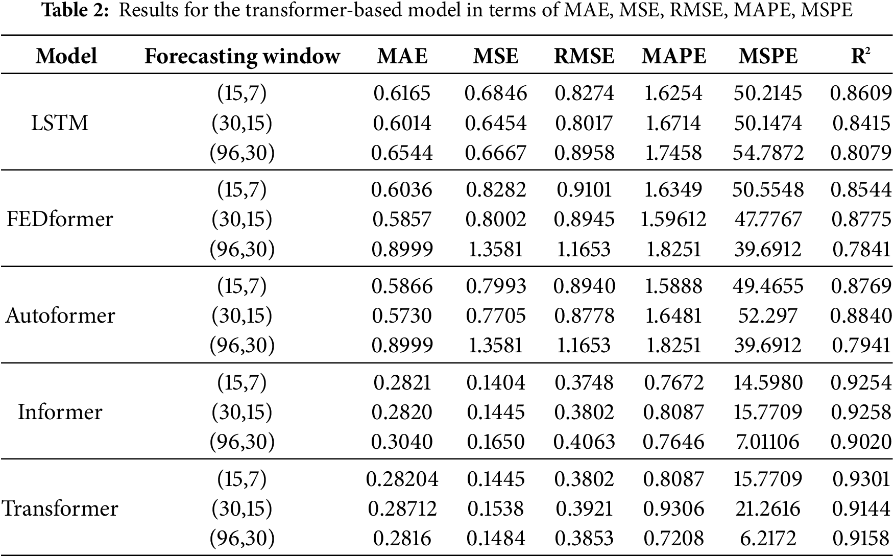
FEDformer performs well with shorter windows (15,7) and (30,15) however experiences performance degradation as the window size increases as can be seen in Table 2. Similarly, Autoformer is effective with shorter windows while underperforming with longer forecasting windows, as with FEDformer. Informer has stable performance with all windows and is especially effective with long forecasting windows, showcasing it as the most robust model among the four. While the transformer is not suitable for short-term forecasting. The LSTM model is also experimented with to provide a comparative analysis with transformer-based models. It can be seen that the LSTM model has not performed well in terms of each evaluation metric as compared to the rest of models.

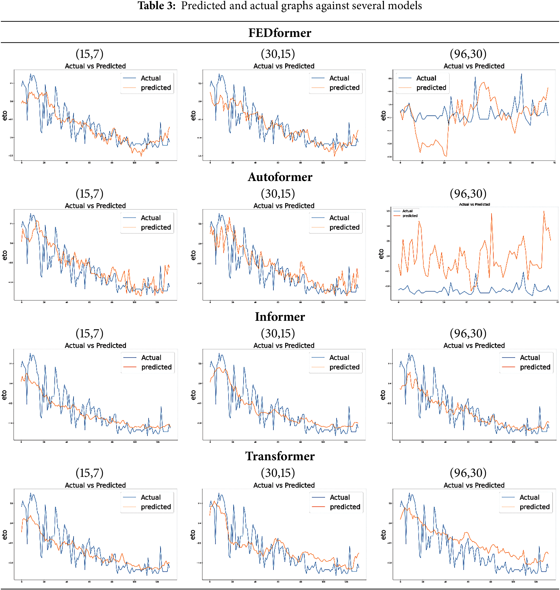
In Table 3, predicted and actual graphs of the model used are displayed. It can be seen that predicted and actual graphs for ETo estimation differ in most cases. However, the informer model has performed best in terms of capturing seasonality. One limitation here is that the informer model does not capture the changes that occur daily, although it achieved very low values for loss metrics such as MSE, RMSE, etc. The rest of the methods capture daily changes; however, the values vary greatly from the actual value that has generated too much loss as in the case of FEDformer and Autoformer. However, the transformer model also generated accurate graphs but is less efficient computationally.

In this section results generated from various methods were discussed and it is concluded that the informer model outperforms others in terms of better efficiency and computational affordability. This study’s results demonstrate the proposed methodology’s effectiveness in improving the accuracy of ETo forecasting. The implications of this study extend beyond ETo forecasting. First, the window-sizing approach, informed by seasonal trends, climatic patterns and empirical testing, provides a framework for handling other multivariate time-series forecasting problems, such as weather prediction, hydrological modeling, and energy demand forecasting. The ability to customize window sizes ensures that models effectively capture temporal dependencies while avoiding overfitting or underfitting issues.

Second, the application of transformer-based architectures like Informer, Autoformer, and FEDformer highlights their suitability for handling large, multivariate datasets with intricate temporal dependencies. These models offer robust alternatives to traditional machine learning and deep learning approaches, especially in domains requiring accurate long-term forecasting. Furthermore, these architectures’ scalability and computational efficiency make them suitable for real-time applications, such as dynamic irrigation scheduling and climate risk assessment.

From a practical perspective, this study has significant applications in agricultural and environmental management. Accurate ETo predictions support optimized irrigation planning, ensuring efficient water use and sustainable crop production. Moreover, the approach can aid policymakers in assessing water resource availability and implementing strategies to mitigate the impact of climate variability on agricultural systems. Additionally, the proposed approach significantly contributes to water resource planning and climate adaptation strategies by enabling accurate and seasonally sensitive ETo forecasting, which is critical for efficient irrigation and reservoir management. The 7-day and 15-day forecast configurations align with practical planning horizons, supporting informed water allocation and reducing risks of over-irrigation or scarcity. Finally, the proposed methodology offers a replicable framework for researchers and practitioners addressing forecasting challenges in other domains. Integrating domain knowledge, data-driven optimization, and cutting-edge architectures provides a blueprint for advancing the state-of-the-art in time-series modeling, paving the way for more reliable and actionable predictions in diverse fields.

The proposed ETo prediction method can be adapted to different geographical contexts by incorporating region-specific climatic and agricultural conditions. Additional meteorological variables like wind speed, soil moisture, or extreme weather indicators can improve accuracy for areas with high climate variability. In arid or semi-arid regions, focusing on drought-related parameters can support better water management, while in contrast regions, refining window sizes to capture short-term fluctuations typical of such climates could enhance performance. The model could also be tailored using localized datasets, including historical climatic records and crop-specific water needs, and integrating geographic information system (GIS) or satellite-based data for regions with sparse ground-level observations.

5  Conclusion

Reference Evapotranspiration (ETo) is a crucial measure of water loss from plant surfaces and land, calculated by setting a reference plant to estimate the water demand for vegetation in a particular environment. Accurate ETo prediction is vital for effective water resource management, especially in agriculture and environmental conservation. This study evaluated four transformer-based architectures—namely, Vanilla Transformer, Informer, Autoformer, and FEDformer—on an ETo dataset from the Andalusian region, aiming to identify which architecture is most suitable for ETo modelling. The experiments demonstrated that the Informer model consistently performed best across various metrics, showing strong predictive accuracy and stability when applied to the dataset. The Vanilla Transformer also showed promising results, ranking second after Informer, likely due to its simpler structure and robustness. Although Autoformer and FEDformer are the most recent advancements in transformer-based architectures, their performance did not match the Informer and Vanilla Transformer on this dataset, possibly due to limitations in adapting to the ETo-specific temporal patterns. Based on these results, future work could focus on developing a hybrid model that combines the strengths of these architectures. By leveraging the predictive capabilities of Informer and Vanilla Transformer with the innovations of Autoformer and FEDformer, a more accurate and efficient model for ETo prediction can be achieved. Such a hybrid model would offer enhanced performance and adaptability, supporting more effective water resource management in agriculture and other fields where ETo modelling is essential. Moreover, detecting extreme weather events or periods of rapid climatic change can enhance prediction capability.

Acknowledgement: This research is supported by Princess Nourah bint Abdulrahman University Researchers Supporting Project, Riyadh, Saudi Arabia. The authors are also thankful to AIDA Lab CCIS Prince Sultan University, Riyadh, Saudi Arabia of APC support.

Funding Statement: This research was funded by Princess Nourah bint Abdulrahman University and Researchers Supporting Project number (PNURSP2024R136), Princess Nourah bint Abdulrahman University, Riyadh, Saudi Arabia.

Author Contributions: The authors confirm contribution to the paper as follows: Conceptualization: Bushra Tayyaba, Muhammad Usman Ghani Khan, Tanzila Saba; Methodology: Talha Waheed, Shaha Al-Otaibi; Software: Bushra Tayyaba, Talha Waheed, Shaha Al-Otaibi; Validation: Tanzila Saba, Muhammad Usman Ghani Khan, Tanzila Saba; Visualization, Writing—review and editing: Bushra Tayyaba, Muhammad Usman Ghani Khan, Talha Waheed, Shaha Al-Otaibi, Tanzila Saba. All authors reviewed the results and approved the final version of the manuscript.

Availability of Data and Materials: The authors confirm that the data supporting the findings of this study are available within the article in Section 2.1.

Ethics Approval: Not applicable.

Conflicts of Interest: The authors declare no conflicts of interest to report regarding the present study.

1https://news.globallandscapesforum.org/50717/everything-you-need-to-know-about-drylands/#:˜:text=Semi%2Darid%20lands%2C%20which%20stretch,aridity%20index%20of%200.2%E2%80%930 (accessed on 05 September 2024).

References

1. Tausif M, Iqbal MW, Bashir RN, AlGhofaily B, Elyassih A, Khan AR. Federated learning based reference evapotranspiration estimation for distributed crop fields. PLoS One. 2025;20(2):e0314921. doi:10.1371/journal.pone.0314921. [Google Scholar] [PubMed] [CrossRef]

2. Gabr ME. Management of irrigation requirements using FAO-CROPWAT 8.0 model: a case study of Egypt. ModelEarth Syst Environ. 2022;8(3):3127–42. doi:10.1007/s40808-021-01268-4. [Google Scholar] [CrossRef]

3. Chapter 2—FAO Penman-Monteith equation. [Online]. [cited 2024 Mar 26] Available from: https://www.fao.org/3/x0490e/x0490e06.htm. [Google Scholar]

4. Feng Y, Cui N, Zhao L, Hu X, Gong D. Comparison of ELM, GANN, WNN and empirical models for estimating reference evapotranspiration in humid region of Southwest China. J Hydrol. 2016 May;536:376–83. doi:10.1016/j.jhydrol.2016.02.053. [Google Scholar] [CrossRef]

5. Agrawal Y, Kumar M, Ananthakrishnan S, Kumarapuram G. Evapotranspiration modeling using different tree based ensembled machine learning algorithm. Water Resour Manag. 2022 Feb;36(3):1025–42. doi:10.1007/s11269-022-03067-7. [Google Scholar] [CrossRef]

6. Youssef MA,Peters RT, El-Shirbeny M,Abd-ElGawad AM, Rashad YM, Hafez M, et al. Enhancing irrigation water management based on ETo prediction using machine learning to mitigate climate change. Cogent Food Agric. 2024 Dec;10(1). doi:10.1080/23311932.2024.2348697. [Google Scholar] [CrossRef]

7. Saggi MK, Jain S. Reference evapotranspiration estimation and modeling of the Punjab Northern India using deep learning. Comput Electron Agric. 2019 Jan;156(9):387–98. doi:10.1016/j.compag.2018.11.031. [Google Scholar] [CrossRef]

8. Kumar U. Modelling monthly reference evapotranspiration estimation using machine learning approach in data-scarce North Western Himalaya region (AlmoraUttarakhand. J Earth Sys Sci. 2023 Sep;132(3):1–15. doi:10.1007/s12040-023-02138-6. [Google Scholar] [CrossRef]

9. Tikhamarine Y, Malik A, Kumar A, Souag-Gamane D, Kisi O. Estimation of monthly reference evapotranspiration using novel hybrid machine learning approaches. Hydrol Sci J. 2019 Nov;64(15):1824–42. doi:10.1080/02626667.2019.1678750. [Google Scholar] [CrossRef]

10. Chen Z, Zhu Z, Jiang H, Sun S. Estimating daily reference evapotranspiration based on limited meteorological data using deep learning and classical machine learning methods. J Hydrol. 2020 Dec;591(7):125286. doi:10.1016/j.jhydrol.2020.125286. [Google Scholar] [CrossRef]

11. Khan AA, Nauman MA, Bashir RN, Jahangir R, Alroobaea R, Binmahfoudh A. Context aware evapotranspiration (ETs) for saline soils reclamation. IEEE Access. 2022;10:110050–63. doi:10.1109/ACCESS.2022.3206009. [Google Scholar] [CrossRef]

12. Salahudin H, Shoaib M, Albano R, Inam Baig MA, Hammad M, Raza A, et al. Using ensembles of machine learning techniques to predict reference evapotranspiration (ET0) using limited meteorological data. Hydrology. 2023 Aug;10(8):169. doi:10.3390/hydrology10080169. [Google Scholar] [CrossRef]

13. Sharma G, Singh A, Jain S. DeepEvap: deep reinforcement learning based ensemble approach for estimating reference evapotranspiration. Appl Soft Comput. 2022 Aug;125(14):109113. doi:10.1016/j.asoc.2022.109113. [Google Scholar] [CrossRef]

14. Vaswani A,Shazeer N, Parmar N, Uszkoreit J, Jones L, Gomez AN,et al. Attention is all you need. Adv Neural Inf Process Syst. 2017;30. [Google Scholar]

15. Dosovitskiy A, Beyer L, Kolesnikov A, Weissenborn D, Zhai X, Unterthiner T, et al. An image is worth 16x16 words: transformers for image recognition at scale. [cited 2024 Mar 26]. Available from: https://arxiv.org/abs/2010.11929 [Google Scholar]

16. Rao Y, Zhao W, Liu B, Lu J, Zhou J, Hsieh C-J. DynamicViT: efficient vision transformers with dynamic token sparsification. Adv Neural Inf Process Syst. 2021 Dec;34:13937–49. [Online]. [cited 2024 Mar 26]. Available from: https://github.com/. [Google Scholar]

17. Wu S, Xiao X, Ding Q, Zhao P, Wei Y, Huang J. Adversarial sparse transformer for time series forecasting. Adv Neural Inf Process Syst. 2020;33:17105–15. [Google Scholar]

18. Zeng A, Chen M, Zhang L, Xu Q. Are transformers effective for time series forecasting? Proc AAAI Conf Artif Intell. 2023 Jun;37(9):11121–8. doi:10.1609/aaai.v37i9.26317. [Google Scholar] [CrossRef]

19. Bellido-Jiménez JA, Estévez J, García-Marín AP. A regional machine learning method to outperform temperature-based reference evapotranspiration estimations in Southern Spain. Agric Water Manag. 2022 Dec;274:107955. doi:10.1016/j.agwat.2022.107955. [Google Scholar] [CrossRef]

20. Zhou H, Zhang S, Peng J, Zhang S, Li J, Xiong H, et al. Informer: beyond efficient transformer for long sequence time-series forecasting. Proc AAAI Conf Artif Intell. 2021 May;35(12):11106–15. doi:10.1609/aaai.v35i12.17325. [Google Scholar] [CrossRef]

21. Wu H, Xu J, Wang J, Long M. Autoformer: decomposition transformers with auto-correlation for long-term series forecasting. Adv Neural Inf Process Syst. 2021 Dec;34:22419–30. [Online]. [cited 2024 Mar 26]. Available from: https://github.com/thuml/Autoformer. [Google Scholar]

22. Zhou T, Ma Z, Wen Q, Wang X, Sun L, Jin R. FEDformer: frequency enhanced decomposed transformer for long-term series forecasting. In: Proceedings of the 39th International Conference on Machine Learning; 2022 Jun 28; PMLR. Vol. 162, p. 27268–86. [Online]. [cited 2024 Mar 26]. Available from: https://proceedings.mlr.press/v162/zhou22g. [Google Scholar]