Real-Time Proportional-Integral-Derivative (PID) Tuning Based on Back Propagation (BP) Neural Network for Intelligent Vehicle Motion Control

1  Introduction

According to recent traffic accident reports, over 1.3 million people die annually in traffic accidents, and this tragic fact highlights the urgent need to enhance the intelligence of traffic safety and control systems. As traffic volume increases and road conditions become more complex, traditional traffic safety management methods are struggling to meet the growing challenges. Control systems are essential for maintaining the efficiency and safety of various processes in modern industrial and technological applications. The effectiveness of these systems directly influences production efficiency, product quality, and operational safety. With the growing level of industrial automation and the widespread adoption of intelligent technologies, the demands on control systems have increased, especially in terms of robustness and adaptability to complex dynamic processes. In parallel, the rise of the Internet of Things (IoT) has driven the evolution of intelligent small-scale vehicles toward greater multifunctionality and diversification. However, these vehicles often face limitations [1] in road analysis and decision-making capabilities, resulting in narrow application scenarios and limited flexibility. Their route planning and road condition analysis abilities are typically weak, leading to reduced practicality.

Despite the extensive use of Proportional-Integral-Derivative (PID) controllers as a classical control method in industrial applications, they exhibit significant limitations when managing nonlinear and time-varying systems. Traditional PID controllers rely on fixed parameter adjustments, which often struggle to adapt to changing system characteristics. This inflexibility can lead to degraded control performance, such as overshooting, oscillations, or slow response times. These limitations become more pronounced when dealing with systems that exhibit strong nonlinearity or complex dynamic behavior, presenting challenges to the effectiveness and stability of control systems.

In response to these challenges, various advanced control strategies have been proposed in recent years. For example, Model Reference Adaptive Control (MRAC) [2], Model Predictive Control (MPC) [3], and fuzzy logic-based controllers [4] have demonstrated significant performance improvements in handling the unpredictable and variable conditions encountered by intelligent vehicles [5]. Additionally, adaptive control methods based on intelligent algorithms have gained considerable attention. Techniques such as fuzzy PID control [6], adaptive PID control [7], neural network-based PID control [8], fuzzy-augmented model-reference-adaptive PID [9], and adaptive fractional-order PID [10] have been extensively studied and applied across different control domains.

In particular, the integration of neural networks in PID control [11] shows great promise due to their powerful nonlinear mapping capabilities [12] and self-learning properties [13]. These features enable neural networks to dynamically adjust PID controller parameters during system operation, significantly enhancing the adaptability and robustness of control systems in complex environments.

This study proposes a novel PID control algorithm based on Backpropagation (BP) neural networks [14] to address the limitations of traditional PID controllers in managing complex dynamic systems. The BP neural network is initially trained to capture the system’s nonlinear dynamic characteristics. It is then seamlessly integrated with the PID controller to form an innovative hybrid control strategy. In this approach, the output states of the neural network’s output layer correspond to the three adjustable parameters (kp, ki and kd) of the PID controller. Through the neural network’s self-learning mechanism and weight adjustments, the PID controller parameters are dynamically optimized. Simulation experiments demonstrate that the proposed BP neural network-based PID design outperforms traditional PID control methods in effectively managing complex systems. Furthermore, the trained model is applied to an intelligent vehicle, with real-world experiments confirming its ability to make timely adjustments under various complex road conditions, maintain consistent vehicle speed, and significantly enhance overall system performance.

The remainder of this paper is organized as follows: The second section explores the dynamics model of a rear-wheel differential electric vehicle, including the design of a wheel dynamics model and the mechanical analysis of individual wheels. The third section introduces the principles of PID control, followed by the design of a PID controller based on BP neural networks, including parameter setting and training, leading to simulation experiments. The fourth section presents the hardware design of the vehicle and the software design for each module. In the fifth section, experiments involving straight-line and curve driving with and without obstacles are conducted, and the results are analyzed. Finally, the sixth section concludes the paper, summarizing the key contributions and findings.

2  Rear-Drive Intelligent Vehicle Dynamics Model

2.1 Problem Description

When a car turns, the outside wheel needs to travel farther than the inside wheel, requiring different speeds for each wheel to prevent instability. Electronic differential control in electric vehicles typically involves two methods: controlling wheel speed or torque [15]. Speed-based control often uses PID and neural networks to track ideal wheel speeds. Torque-based control [16], meanwhile, incorporates vehicle yaw motion control to optimise torque distribution for stability. Vehicle stability control has evolved from basic systems in the 1990s to methods directly applying force to wheels, marking a new chapter in car stability [17].

2.2 Dynamic Modeling

The primary focus of this chapter is on the dynamics model of the rear-wheel differential electric vehicle. To achieve stability control of the car, developing a computer model for conducting relevant theoretical research and simulation experiments is essential. A suitable vehicle dynamics model forms the foundation of this research. The chapter begins by establishing the kinematics model of the three-wheel intelligent vehicle, progressing from individual components to the entire system. Then, the vehicle dynamics model is synthesised.

2.2.1 Establishment of Kinematics Model of Three-Wheeled Intelligent Vehicle

The three-wheel intelligent vehicle [18] features a front driving wheel configured as a universal wheel while the rear driving wheel’s axle is aligned [19]. Each rear wheel is independently controlled by its motor. One wheel in front of the car governs the steering of the vehicle, whereas the rear wheels control its movement by adjusting speed, resulting in a combination of rolling and sliding motion. The wheeled intelligent vehicle’s chosen center is the rear axle’s midpoint. Fig. 1 illustrates the structural diagram of the intelligent vehicle in motion.

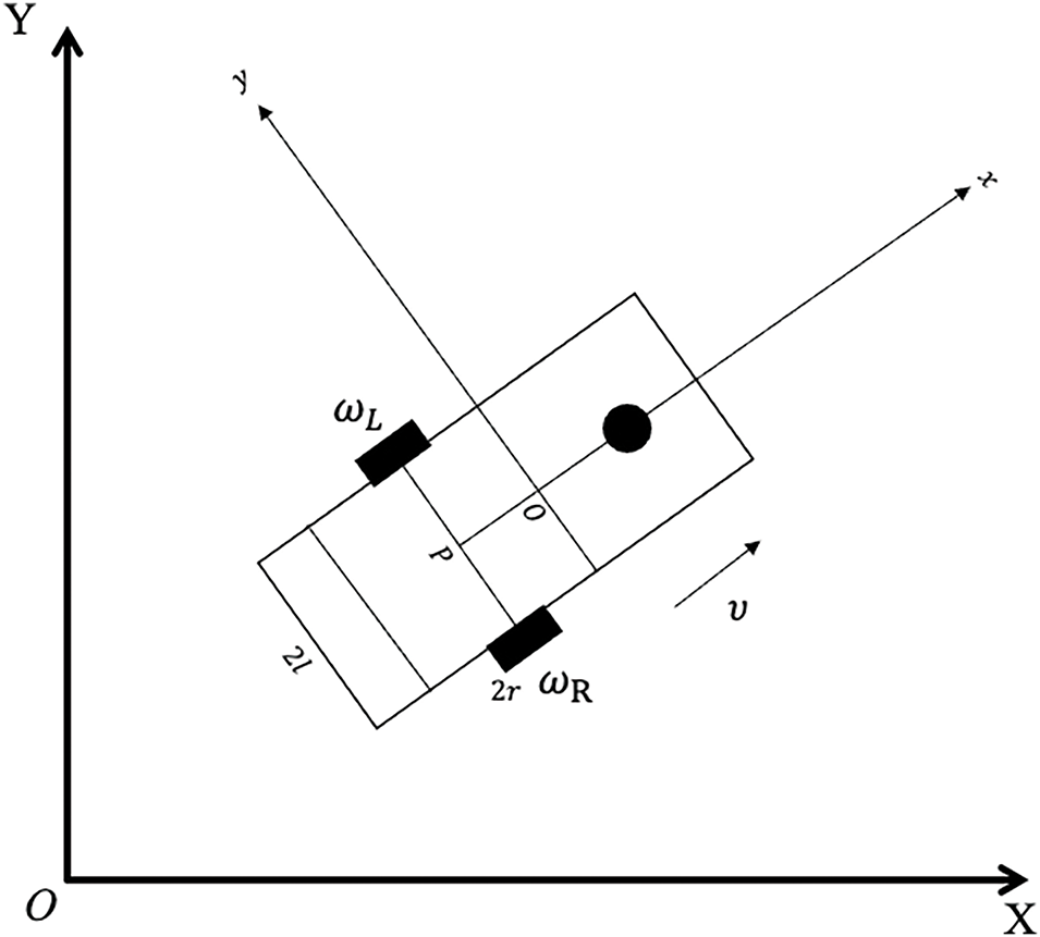
Figure 1: Movement structure of the intelligent vehicle

In Fig. 1, the local coordinate system was represented by the coordinate system X-O-Y, while the coordinate system X-O-Y represented the global coordinate system, the coordinates of the centroid were denoted as p(xp,yp), the coordinates of the center of mass were represented as o(x,y), and θ indicated the heading angle of the intelligent vehicle. The main kinematic parameters of wheeled intelligent vehicles are shown in Table 1:

Set the left driving wheel’s angular velocity when it moves as wL and the angular velocity of the right driving wheel as wR. According to the geometric relationship of the intelligent vehicle in Fig. 1, the following constraint equation can be obtained:

{x1˙cos⁡θ+y1˙sin⁡θ−lθ˙=rωLx1˙cos⁡θ+y1˙sin⁡θ+lθ˙=rωR−x1˙cos⁡θ+y1˙sin⁡θ+dθ˙=0(1)

In the provided equations, the first two equations represent pure rolling constraints applied to the intelligent vehicle, ensuring the driving wheel’s smooth sliding. Among the three constraint equations, one is a complete constraint, while the other two are non-complete constraints.

The mobile robot’s linear speed when moving is expressed by v, and the angular speed is expressed by ω, and the speed equation of the intelligent car when moving can be obtained:

{v=vL+vR2=(ωL+ωR)r2θ˙=ω=r2l(ωR−ωL)(2)

2.2.2 Establishment of Vehicle Dynamics Model

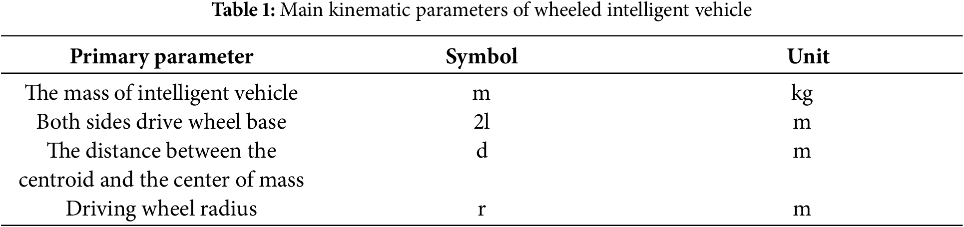
In the path tracking process of the rear-wheel differential electric vehicle, to denote the current position coordinates of the car [20], we assume the geodetic coordinate system as XOY, the vehicle coordinate system as XOY, and φ is the vehicle yaw angle, as depicted in Fig. 2.

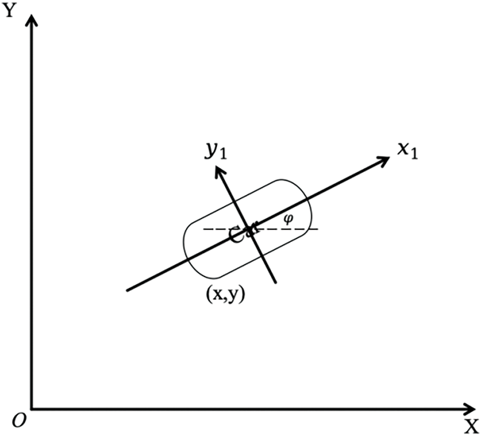
Figure 2: Vehicle geodetic coordinate reference system

The motion equation of the vehicle in the geodetic coordinate system can be expressed as:

X1=x1cosφ−y1sinφY1=x1sinφ−y1cosφ(3)

3  PID Controller Design Based on BP Neural Network

3.1 PID Control Principle

In the control system, the most common control law of the controller is PID control. The analogue PID control system’s principle framework is illustrated in Fig. 3. The system is comprised of an analogue PID controller as well as a controlled object. It is divided into three modules: proportion, differentiation, and integration. The control law is output in real-time by the difference between the actual output and the controlled object’s expected output.

Figure 3: Schematic diagram of analog PID control system

PID is a linear controller, which constitutes a control deviation according to the given value rin(t) and the actual output value yout(t), as illustrated in Formula (4).

error(t)=rin(t)−yout(t)(4)

PID control rule is as follows:

u(t)=kp(error(t)+1T1∫0terror(t)dt+TDderror(t)dt)(5)

Or written as a transfer function:

G(s)=U(s)E(s)=kp(1+1T1s+TDs)(6)

where kp—scale coefficient, T1—integral time constant; TD—differential time constant.

In simple terms, the functions of each PID controller correction link are as follows:

(1)   Proportional link: It is proportionate to the error signal error(t) of the control system. Once a deviation occurs, the controller promptly generates a control effect to minimize the deviation.

(2)   Integral link: Primarily used to eliminate static errors and enhance the system’s accuracy. The effectiveness of the integral action is determined by the integral time constant T1. A higher T1 weakens the integral action, and vice versa.

(3)   Differentiation: Reflects the change trend (rate of change) of the deviation signal. It can introduce an effective early correction signal into the system before the deviation signal grows too large, accelerating the system’s response speed and reducing adjustment time.

3.2 Simulation Experiment of Classical Linear PID Control

As can be seen from Formula (6), the PID control rule can be written as a transfer function. The fist-order inertia system transfer function as shown in Formula (7) was used.

G(s)=0.9980.021s+1(7)

The reason for selecting this transfer function was because a first-order inertia system served as a simplified model for many real-world systems, such as thermal systems and mechanical systems. Therefore, opting for such a transfer function can encompass a wide range of practical applications, effectively showcasing the fundamental characteristics of control systems and the performance of control algorithms.

In the present conventional linear PID simulation experiment, the parameters kp=0.22, ki=0.13 and kd=0 were selected. These values were chosen to achieve rapid system response, minimize steady-state error, and ensure the stability of the control system.

After setting the parameters, the simulation experiment was conducted as shown in Fig. 4. Fig. 4a displayed the system response with classical PID control, showing the reference signal (red dashed line) and the output response (blue solid line) over time. Fig. 4b represented the tracking error over time. It depicted the deviation between the reference signal and the actual output of the system. In both figures, it was evident that around 0.25 s, the system’s output reached the desired value of 1, while the tracking error diminished to zero.

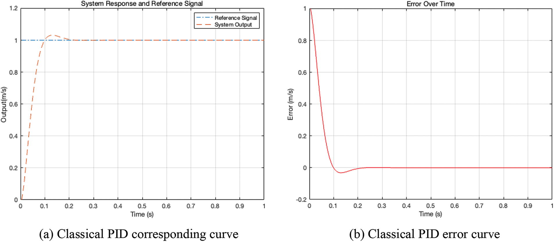
Figure 4: Classical linear PID curve

The experiment results indicated that the classical linear PID control required manual adjustment of three parameters, which was time-consuming and challenging, especially in complex systems. Moreover, the classical linear PID control may take a long time to bring the system to the desired setpoint, yielding suboptimal results, particularly in scenarios simulating the actual movement of vehicles.

3.3 PID Design Based on BP Neural Network

In PID control, it is necessary to adjust the proportional, integral and differential three kinds of control action to get a better control effect. The formation of control quantity both cooperates and restricts each other. This relationship is not necessarily a simple “linear combination”. From the infinite nonlinear combination, we can find the best relationship. The optimal combination of PID control can be realized by learning the performance of the system because of the ability to perform an arbitrary nonlinear expression of the neural network. Using the BP network, the self-learning PID controller with parameters kp, ki and kd can be established.

The PID control system’s structure based on the BP network is illustrated in Fig. 5. The controller comprises two parts:

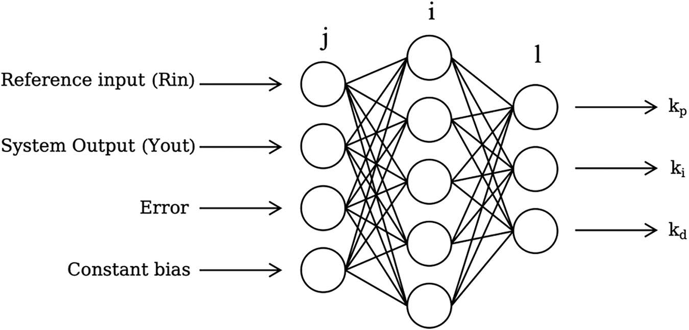
Figure 5: BP neural network structure

(1)   The classical PID controller can control the controlled object directly, kp, ki and kd are adjusted online.

(2)   The neural network adjusts the parameters of the PID controller according to the operating state of the system to achieve the optimization of specific performance indicators so that the output state of the neurons in the output layer corresponds to the three adjustable parameters of the PID controller kp, ki and kd through the self-learning and weighting coefficient adjustment of the neural network. The neural network output corresponds to the PID controller parameters under some optimal control.

The control algorithm of the classic incremental digital PID is

u(k)=u(k−1)+kp(error(k)−error(k−1))+kierror(k)+kd(error(k)−2error(k−1)+error(k−2))(8)

In the formula, kp, ki and kd are proportional, integral and differential coefficients, respectively.

A three-layer BP neural network is adopted, and its structure is shown in Fig. 5.

The input in the input layer of the network is

Oj(1)=x(j)j=1,2,⋯M(9)

In Formula (9), the number of M depends on the complexity of the controlled system.

The input and output of the hidden layer are

neti(2)(k)=∑j=0Mwij(2)Oj(1)Oi(2)(k)=f(neti(2)(k))(i=1,⋯Q)(10)

where wij(2) represents the weighting coefficient of the hidden layer. The labels (1)–(3) denote the input layer, hidden layer, and output layer, respectively.

The activation function in the hidden layer is a Sigmoid function with positive and negative symmetry:

f(x)=tanh⁡(x)=ex−e−xex+e−x(11)

The input and output of the network output layer are

neti(3)(k)=∑i=0Qwli(3)Oi(2)(k)Ol(3)(k)=g(netl3(k))(l=1,2,3)O1(3)(k)=kpO2(3)(k)=kiO3(3)(k)=kd(12)

The output nodes of the output layer correspond to three adjustable parameters. kp, ki and kd, respectively. Since kp, ki and kd cannot be negative, the activation function of neurons in the output layer is a non-negative Sigmoid function.

g(x)=12(1+tanh⁡(x))=exex+e−x(13)

Take the performance indicator function as

E(k)=12(rin(k)−yout(k))2(14)

The weight coefficient of the network is modified according to the gradient descent method. That is, the negative gradient direction of the weight coefficient is searched and adjusted according to E(k), and an inertial term is added to make the search convergence fast and globally minimal.

Δwh(3)(k)=−η∂E(k)∂wh(3)+αΔwli(3)(k−1)(15)

where η is the learning rate, α is the inertia coefficient

∂E(k)∂wh(3)=∂E(k)∂y(k)⋅∂y(k)∂u(k)⋅∂u(k)∂Ol(3)(k)⋅∂Ol(3)(k)∂netl(3)(k)⋅∂netl(3)(k)∂wh(3)(k)(16)

∂netl(3)(k)∂wh(3)(k)=Oi(2)(k)(17)

Since ∂y(k)∂u(k) is unknown, the approximation is replaced by the symbolic function sgn(∂y(k)∂u(k)), and the resulting inaccuracy can be compensated by adjusting the learning rate.

It can be obtained by Formulas (8) and (12).

∂u(k)∂O1(3)(k)=error(k)−error(k−1)(18)

∂u(k)∂O2(3)(k)=error(k)(19)

∂u(k)∂O3(3)(k)=error(k)−2error(k−1)+error(k−2)(20)

The learning algorithm of the network output layer weight obtained from the above analysis is

Δwli(3)(k)=αΔwli(3)(k−1)+ηδl(3)O1(2)(k)(21)

δi(3)=error(k)sgn(∂y(k)∂u(k))∂u(k)∂Ol(3)(k)g′(netl(3)(k))(l=1,2,3)(22)

Similarly, the learning algorithm of the weighting coefficient of the hidden layer can be obtained:

Δwij(2)(k)=αΔwij(2)(k−1)+ηδl(2)Oj(1)(k)(23)

δ1(2)=f(neti(2)(k))∑l=13δl(3)wli(3)(k)(i=1,2,⋯Q)(24)

where g′(⋅)=g(x)(1−g(x)),

f′(⋅)=(1−f2(x))/2(25)

The PID controller structure based on the BP neural network is shown in Fig. 6. The control algorithm of the controller is summarized:

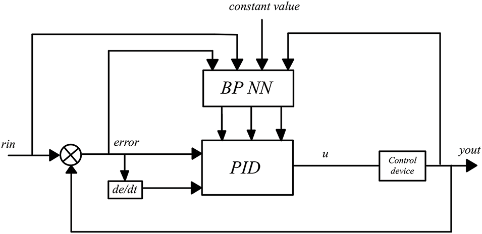
Figure 6: PID controller structure based on BP neural network

(1) Determine the structure of the BP network by establishing the number of nodes in the input layer (M) and the number of nodes in the hidden layer (Q). Assign initial values to the weighted coefficients of each layer wij1(0) and wli2(0), select the learning rate (η), and determine the inertia coefficient (α) with k = 1.

(2) rin(t) and yout(t) are obtained by sampling, and error(k)=rin(t)−yout(t) is calculated at this time.

(3) Calculate neurons’ input and output in each layer of neural network NN, and the NN output layer’s output is the three adjustable parameters kp, ki and kd.

(4) Calculate the output u(k) of the PID controller.

(5) Carry out neural network learning, adjust the weighted coefficients wij1(k) and wli2(k) online, and realise the adaptive adjustment of PID control parameters.

(6) Set k = k + 1 and return to (1).

3.4 Parameter Setting and Training

As can be seen from Formula (11), the Learning Rate determines the updating degree of model parameters in each iteration. A larger learning rate [21] will make the model move a larger step in the direction of gradient descent in each iteration, and the convergence speed will be faster, but shock or instability may occur. Smaller learning factors make the model convergence slower but more stable and robust. In the experiment, when the learning factor was 0.28, the model may had a faster convergence rate as shown in Fig. 7.

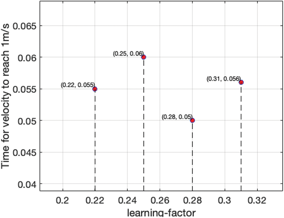
Figure 7: Selection experiment of learning-factor

The inertia factor determines the inertia of the model update, that is, the degree of impact of the last parameter update. A larger inertia factor will increase the inertia of model parameter updating, which makes the model more convergent at high speed and has a certain degree of noise robustness. However, it is also prone to oscillation and instability. A smaller inertia factor will reduce the inertia of parameter updating and thus reduce the convergence rate of the model, but it is generally stable. In the experiment, when the inertia factor was 0.04, the model may had a faster convergence rate and was relatively stable, but there may be some overfitting phenomenon.

Let the controlled object’s approximate mathematical model be

yout(k)=a(k)yout(k−1)1+yout2(k−1)+u(k−1)(26)

where the coefficient a(k) is slightly time-varying, a(k) = 1.2*(1 − 0.8*e−0.1k).

The learning rate determines the updating degree of model parameters in each iteration, and the smaller learning factor makes the model convergence slower but more stable and robust. After many tests, the learning efficiency is 0.28. The inertia coefficient determines the inertia of the model update, that is, the degree of influence produced by the last parameter update. A smaller inertia factor will reduce the inertia of parameter updating, thus reducing the convergence speed of the model, but it is usually relatively stable. The inertia coefficient is 0.05, and the initial value of the weighting coefficient is a random number in the interval [−0.5, 0.5] of [x]. Input command signals are categorised:

rin(t)=1.00.

rin(t)=sin(2πt).

When S = 1 is used as step tracking when S = 2 is used as sine tracking, the weight at the beginning is used as a random value, and the unchanged weight is used to replace the random value after the stable operation.

3.5 Simulation Experiment on BP-PID

The tracking results and corresponding curves were illustrated in Fig. 8.

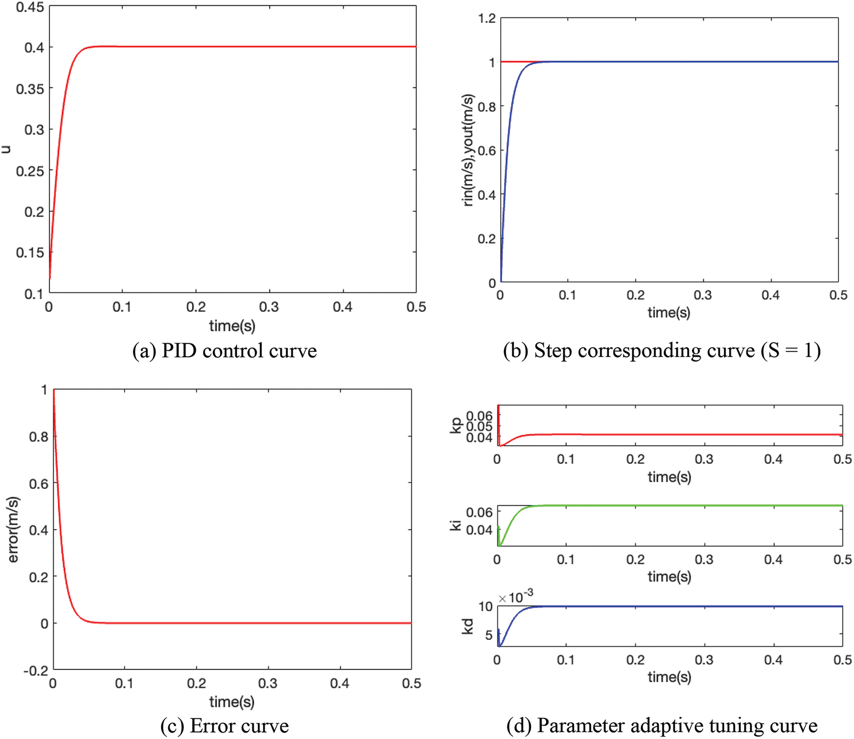
Figure 8: PID curve based on BP neural network

Fig. 8 demonstrated successful speed control without overshoot, with the error approaching zero and the parameters adjusting adaptively to maintain stable performance. The expected speed was represented by a step signal, while the real-time output speed of the car was also displayed. At 0.065 s, the output speed of the car reached 1 m/s and subsequently remained steady at 1 m/s over time, with no overshoot observed. The error diagram shown that at 0.065 s, the error tended towards zero, and as time progressed, the error remained zero, indicating effective tracking of the desired speed. Additionally, the parameter adaptive tuning curves illustrated the changes in kp, ki and kd parameters over time. Initially, when the error was large, the parameters fluctuated significantly; however, they stabilized as the error approaches zero at 0.065 s.

In this section, a speed tracking experiment was conducted where the speed followed a sine wave curve over time. As illustrated in Fig. 9, the expected speed exhibited a sinusoidal distribution as time progresses, and the car’s output speed tracked the expected speed in real time. The PID control quantity curve showcased how the control quantity changes dynamically over time to effectively regulate the car’s speed. The error curve highlighted the variation in error over time, indicating that, unlike the step signal, the error for the sine wave signal constantly fluctuated, showing the car’s continuous effort to track the desired sine wave speed under PID control. Additionally, the parameter adaptive output tuning curve demonstrated how the three parameters kp, ki and kd adjust in real-time, ultimately enabling effective tracking of the desired speed.

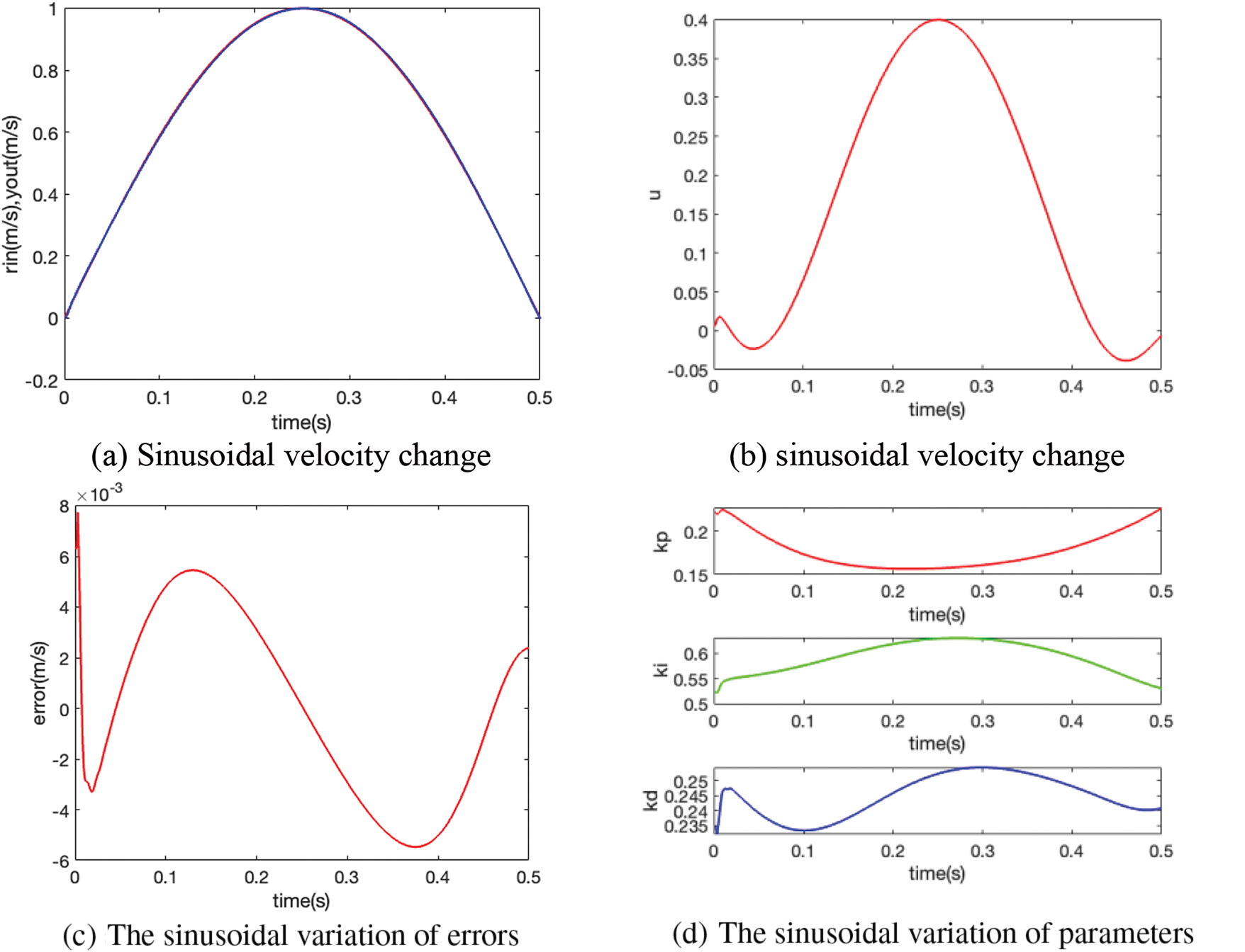
Figure 9: The speed tracking experiment following a sine wave curve

3.6 Comparison of PID Algorithm Based on BP Neural Network and Traditional PID Algorithm

Through the traditional PID simulation experiment in Section 3.2 and the BP-based PID algorithm in Section 3.5, the data of the two experiments are recorded in Table 2.

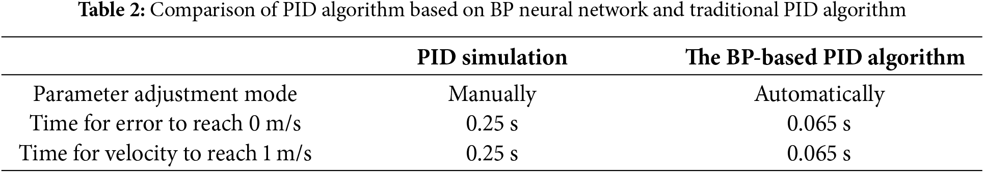
Overall, these figures collectively demonstrate the successful implementation of the BP-PID algorithm in ensuring the vehicle effectively tracks the desired speed. By following a sinusoidal trajectory, it can be concluded that the BP-PID algorithm, based on neural networks, can adaptively adjust PID parameters according to system behavior, thereby enhancing performance and robustness. Additionally, the comparative data from the traditional linear PID simulation experiments in Section 3.2 shows that the BP-PID algorithm reduces the time required to reach the target speed by 74.0%.

4  Visual Navigation and System Hardware and Software Design

The PID algorithm based on BP neural network can be combined with many other practical functions. This section will combine the PID algorithm based on BP neural network with the smart home vehicle to explore its performance. In this section, Section 4.1 introduces 14 hardware designs of the vehicle system, analyses and selects each hardware, and finally shows the overall prototype of the system. Section 4.2 introduces the software design of the vehicle system, including various functional modules and system software framework.

The main control hardware design is shown in Fig. 10. The STM32 microcontroller [22] can utilize a BP neural network-based PID control system to regulate the operation of two motors, while enabling real-time feedback and control of each module’s functionality through Bluetooth and WIFI remote control. The main control microcontroller can achieve automatic control based on feedback from environmental monitoring data, as well as operate according to user settings.

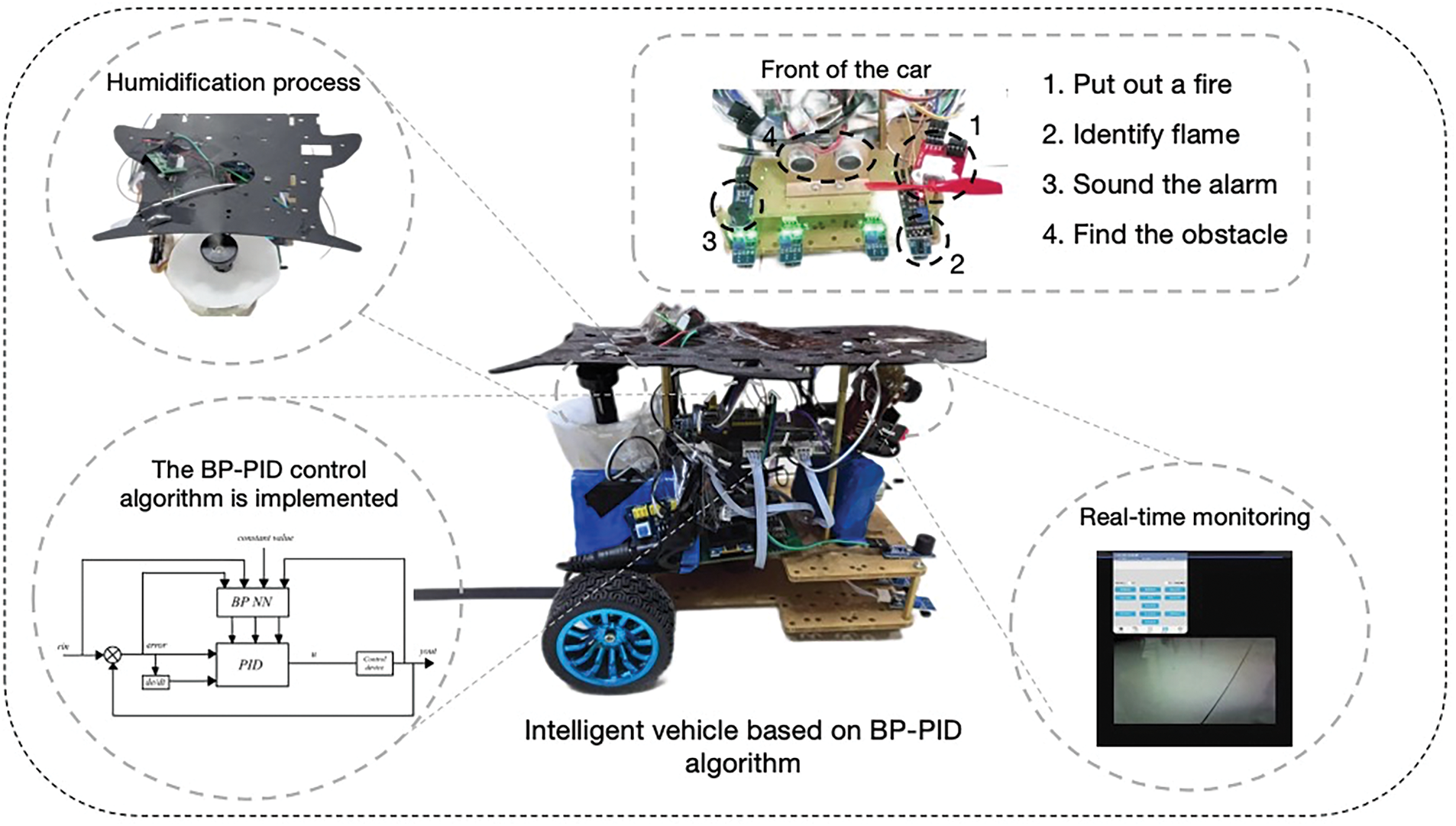
Figure 10: The main control hardware design

4.1 Vehicle Hardware Design

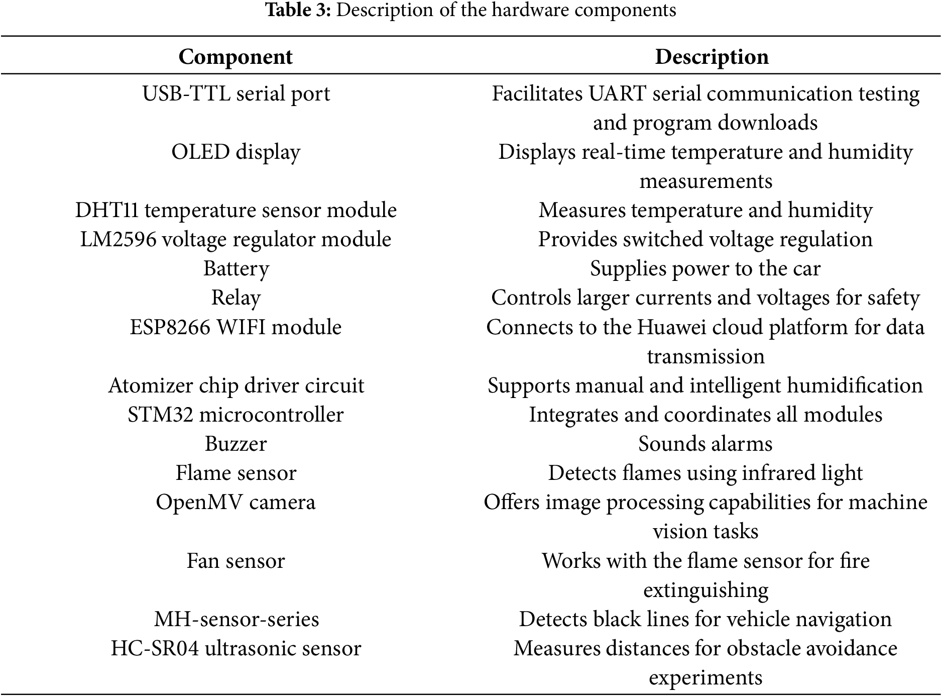
There are 15 kinds of hardware in this system as shown in Table 3, including USB-TTL serial port [23], OLED display screen [24], DHT11 temperature sensor module [25], LM2596 voltage regulator module, Battery [26], Relay, ESP8266 WIFI module [27], Atomizer chip driver circuit, STM32 microcontroller [28], Buzzer, Flame sensor, the OpenMV camera, Fan sensor, MH-Sensor-Series and HC-SR04 Ultrasonic Sensor.

4.2 Overall System Prototype

The overall system is shown in Fig. 11. In front of the system are four infrared sensor modules that identify black line tracking [29]. The fire extinguishing device system [30] is located in the upper part and consists of a flame-sensing module, a buzzer, and a fan sensor module. The ultrasonic ranging module is located in the middle of the front of the system. It can emit ultrasonic waves to measure the distance from the front obstacles to achieve obstacle avoidance [31]. Behind the ultrasonic module is a PCB board with multiple peripheral modules and an STM32 chip master. The DHT11 module can detect the current indoor temperature and humidity, an OLED display can display the measured temperature and humidity in real-time, and an ESP8266 WI-FI module is used to connect to WI-FI and connect to the Cloud platform [32] through WI-FI [33] to achieve intelligent temperature and humidity control.

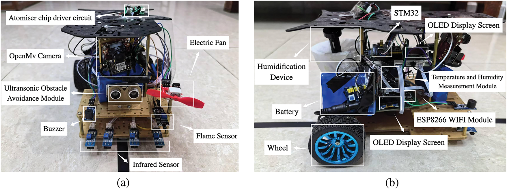
Figure 11: Overall prototype of the system

Finally, at the rear of the system, there is an atomisation plate driver module, which enables the product to complete the manual humidification function. When combined with the Huawei Cloud Platform, the intelligent humidification switch function can be realised. Below are two coding motors and two wheels. Two coding motors can be coded for PID control, which can make the car more stable to drive.

4.3 Vehicle System Software Design

(1) Infrared Line-Following Module

The system integrates an infrared line-following functionality, enabling the intelligent vehicle to autonomously navigate along predefined paths marked by contrasting colors, such as black lines on a white surface as shown in Fig. 12. When this function is activated, the vehicle utilizes infrared sensors to detect the presence of the line and adjusts its course accordingly to stay on track.

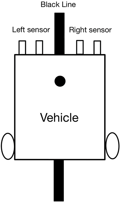
Figure 12: Left and right infrared sensor configuration diagram

The infrared sensors emit infrared light and measure the reflection from the surface beneath. When the sensors detect a higher reflection intensity, indicating a white surface, the vehicle recognizes that it is off the line and adjusts its movement to correct its trajectory. Conversely, when the sensors detect lower reflection intensity from the black line, the vehicle maintains its course.

In the line-following mode, the system continuously monitors the sensor readings to determine the vehicle’s position relative to the line. If the vehicle drifts away from the line, the control system processes the sensor data and adjusts the wheel speeds to steer the vehicle back onto the line. For example, if the left sensor detects the line and the right sensor does not, the vehicle will slow down the right wheel while increasing the speed of the left wheel to turn left and re-align with the line.

Users also have the option to switch to manual mode, allowing for direct control of the vehicle’s movement if desired. This flexibility ensures that the vehicle can be operated in various environments and conditions.

To implement this functionality, we established a microcontroller-based control unit that processes the sensor data in real time. The infrared line-following module effectively enhances the vehicle’s ability to navigate autonomously, ensuring it follows the designated path accurately.

The overall process of the infrared line-following module is illustrated in Fig. 12, showcasing the interaction between the sensors, control unit, and vehicle movement adjustments. Furthermore, this module lays the groundwork for the linear and curve experiments detailed in Section 5.1, ensuring effective line following.

(2) Obstacle Avoidance Module

This module employs an ultrasonic sensor to detect obstacles using sound wave reflection characteristics. The sensor emits ultrasonic waves and measures the time it takes for the waves to bounce back after hitting an object as shown in Fig. 13. By calculating the distance to the obstacle based on the time delay, it provides real-time data to the control system, enabling quick responses to potential collisions. The distance to the obstacle is calculated using the following formula:

D=C×T2(27)

where D represents the calculated distance to the obstacle, C is the speed of sound in air (approximately 343 m/s under standard conditions), and T denotes the time taken for the ultrasonic wave to travel to the obstacle and return.

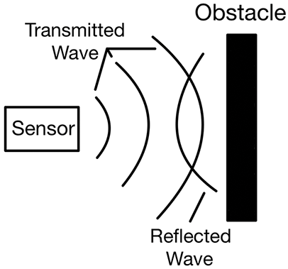
Figure 13: Schematic diagram of ultrasonic obstacle avoidance module

The ultrasonic sensor operates at a frequency of approximately 40 kHz, with a detection range typically between 2 cm and 4 m. Its detection angle is around 30°, allowing it to effectively sense obstacles within a specified field of view. This capability makes it particularly useful for dynamic environments where obstacles may appear suddenly.

When an obstacle is detected within a predefined threshold (e.g., 30 cm), the sensor generates a digital signal indicating the presence of an obstacle. This signal is transmitted to the intermediate processor, which performs programmed logic to determine the appropriate avoidance maneuver. The processor interprets the distance and location of the obstacle to decide whether to steer left, right, or reverse, depending on the obstacle’s position relative to the vehicle’s path.

If the obstacle is directly in front of the vehicle, the system may initiate a reverse maneuver followed by a turn to the right or left to navigate around the obstacle. In cases where multiple obstacles are detected, the processor prioritizes the closest one, ensuring that the vehicle takes the safest and most efficient path.

Additionally, the obstacle avoidance system includes a feedback loop, where continuous monitoring allows for real-time adjustments to the vehicle’s trajectory. This ensures that once the obstacle is bypassed, the system will check the path ahead before returning to the original route, maintaining smooth navigation.

Overall, this ultrasonic-based obstacle avoidance module significantly enhances the intelligent vehicle’s ability to operate safely in unpredictable environments, thereby preventing accidents and improving overall operational efficiency. Furthermore, it lays a solid foundation for the obstacle avoidance experiment detailed in Section 5.2, demonstrating its practical application and effectiveness in real-world scenarios.

(3) Bluetooth Control Module

The intelligent car is an autonomous robot capable of driving and performing tasks independently. Utilising a Bluetooth module, it communicates via 2.4 GHz radio waves, enabling interaction and control with mobile phones and other electronic devices, facilitating various actions such as forward, backwards, turning, patrolling, and task execution. During other operations, client control can forcefully interrupt the ongoing action and execute the provided command.

The Bluetooth module is a crucial communication component between the smart car and mobile phones. It comprises a Bluetooth chip and associated circuit connections, establishing a Bluetooth connection between the intelligent vehicle and mobile phone. Typically, smart cars employ Bluetooth 2.0 or higher modules to achieve enhanced data transmission rates and stability.

Control commands transmitted from the mobile phone to the smart car through the Bluetooth module dictate corresponding actions, including forward, backwards, turning, and task execution. The intelligent vehicle dynamically adjusts its state and behaviour based on received instructions.

The Bluetooth module decodes instructions from the mobile phone and transmits them to the smart car’s control system. Subsequently, the control system processes and executes the instructions that were received. Concurrently, the smart car can transmit status updates and sensor data to the mobile phone through the Bluetooth module, facilitating real-time monitoring and feedback.

5  Experiment and Analysis

After several training iterations, the car relied on the trained model to perform line patrol using the four front infrared tubes with high accuracy. Additionally, it effectively avoided obstacles by utilizing the front ultrasonic ranging module. The experiments in this section were categorized into navigation experiments without obstacles, which encompass straight-line and curve experiments, and navigation experiments with obstacles, including static and moving obstacle experiments.

5.1 Navigation Experiment without Obstacles

(1) Linear experiment

In line inspection, when the four infrared pairs in front of the car did not detect black lines, the vehicle moved forward, as shown in Fig. 14a.

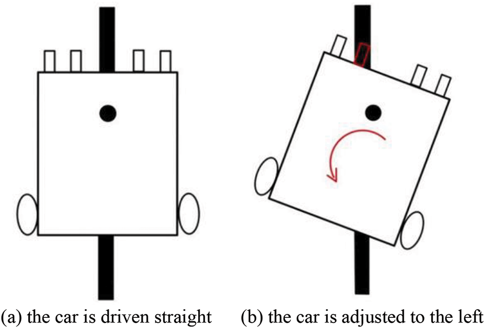
Figure 14: Schematic diagram of straight-line driving

When the car experienced a slight deviation from the straight line, the left and right infrared tubes positioned in the middle of the vehicle accurately identified the black line and initiate corresponding minor adjustments in the appropriate direction. For instance, if the left infrared pair tube detected a black line, the car rotated slightly to the left using the speed difference between the two wheels (with speeds set at 4 m/s for the left wheel and 6 m/s for the right wheel), as depicted in Fig. 14b. Eventually, when none of the four infrared pair tubes detected a black line, the car continued running in a straight line.

In order to test the time required for a car with BP-PID algorithm to travel in a straight line compared to a car with conventional PID algorithm, the vehicle travelled in a straight line without obstacles. As shown in Fig. 15, the car started at the starting point and kept going.

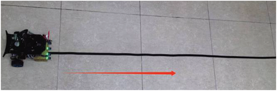
Figure 15: Schematic diagram of linear experiment

Fig. 16 illustrates the car’s movement from the starting point to the endpoint. The car moved forward smoothly, but due to the smoothness of the ground or varying friction coefficients between the two tires, it deviated slightly to the left in Fig. 16-3. The car then made minor adjustments to the right, ensuring that no further deviation from the straight path occurred for the remainder of the experiment. With the car speed set to 5 m/s, the measurement results for different algorithms used by the car are presented in Table 4. As shown in Table 4, the car using BP-PID algorithm consistently maintained a speed of approximately 4.25 m/s across varying linear driving distances, even with minor adjustments.

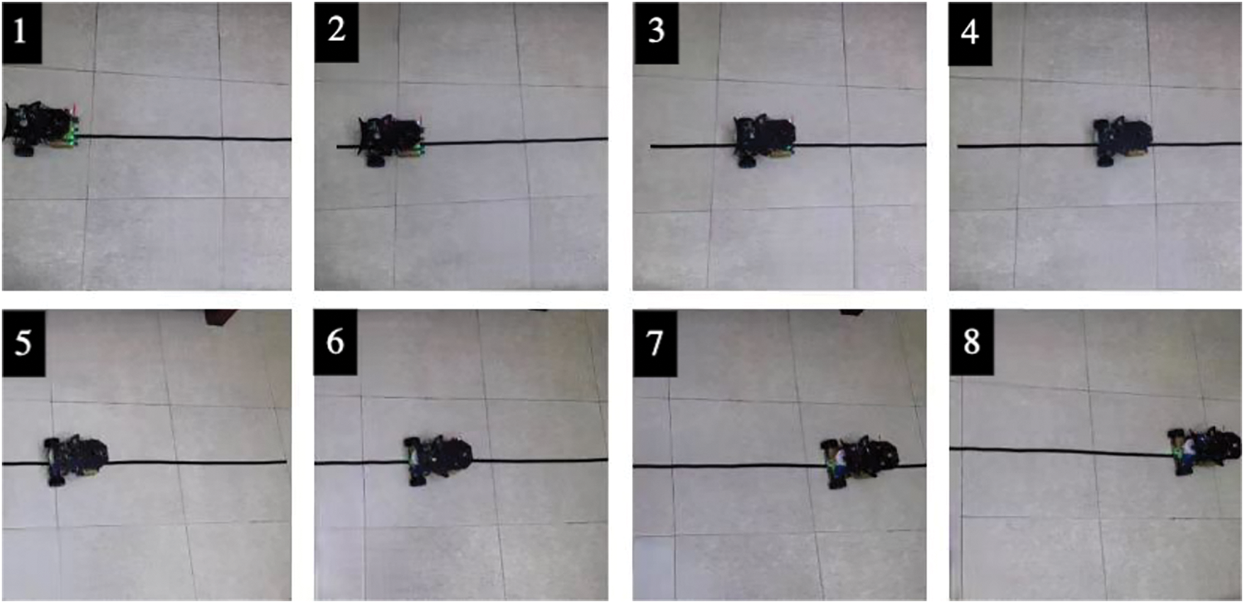
Figure 16: Linear experiment process

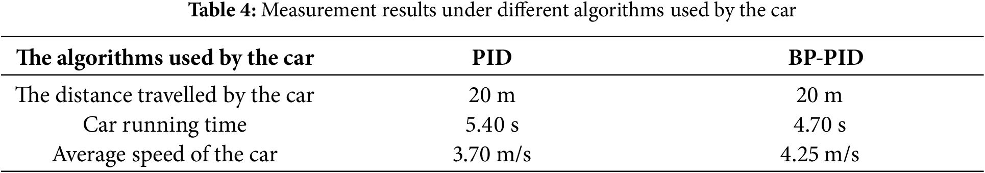
Overall, the linear experiment shown that the car equipped with the BP-PID algorithm required 0.7 s less time to cover the same distance compared to the car using the traditional PID algorithm, and its speed increased by 0.55 m/s, as shown in Table 4. Furthermore, the data in Table 4 demonstrates that the BP-PID-equipped car outperformed the traditional PID-equipped car over longer distances, exhibiting faster and more stable performance. This was because the BP neural network continuously adjusted the weights and biases of the network based on the error between the system’s output and the desired value, using the backpropagation mechanism. These adjustments directly influenced the updating of the PID parameters, allowing the kp, ki and kd values to adapt in real-time to changes in the system.

(2) Curve experiment

The middle two infrared pairs were utilized in the straight-line experiment, whereas all infrared pairs were employed in the curve experiment. The operational principle remained consistent across both experiments. Fine-tuning occurred at the corresponding position when the two middle infrared pairs detected black lines. Subsequently, the car utilized the speed difference between the two wheels (with speeds set at 6 m/s for the left wheel and 4 m/s for the right wheel) to execute a slight right rotation, as depicted in Fig. 17a.

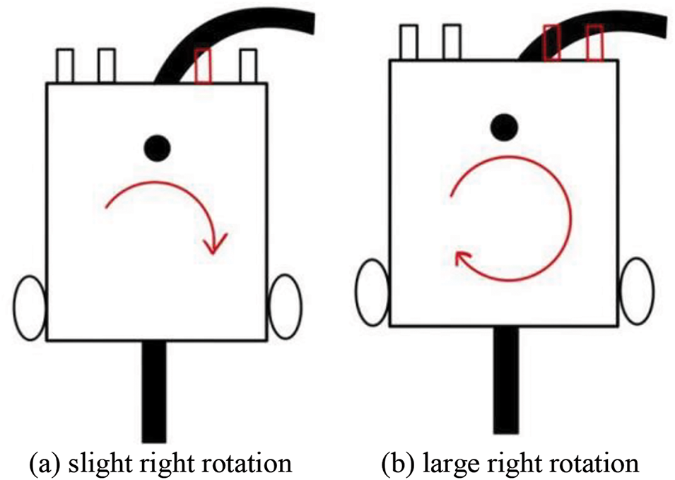
Figure 17: Schematic diagram of curve experiment

During the curve experiment, significant adjustments were made at the corresponding positions when the two outer infrared pairs detected the black line. For instance, if the infrared pair on the right side of the middle of the vehicle detected a black line, the car rotated substantially to its right by modulating the speed difference between the two wheels (with speeds set at 8 m/s for the left wheel and 2 m/s for the right wheel), as illustrated in Fig. 17b.

To test the car’s curve driving time, we found that the car performed curvilinear driving without encountering obstacles. To ensure the accuracy of the experiment, the 90-degree turning angle was measured multiple times to verify the car’s turning precision. Experiment (2), as shown in Fig. 18, confirmed the accuracy of the car when making turns at approximately a 90-degree angle.

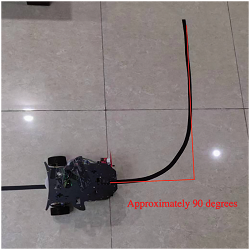
Figure 18: Schematic diagram of curve experiment

As depicted in Fig. 19, the car commenced from the starting point illustrated in Fig. 19-1. Upon encountering the corner shown in Fig. 19-2, the car executed a slight left adjustment before navigating the corner depicted in Fig. 19-3. Subsequently, the car continued forward until it detected a black line in Fig. 19-4. At this point, the car made another small adjustment to the left before navigating the corner depicted in Fig. 19-5 and continuing straight ahead. The car underwent another left adjustment, as shown in Fig. 19-7, before reaching the endpoint successfully, as illustrated in Fig. 19-8. Throughout its journey, the car effectively manoeuvred through corners and aligned with the black line to progress along its path.

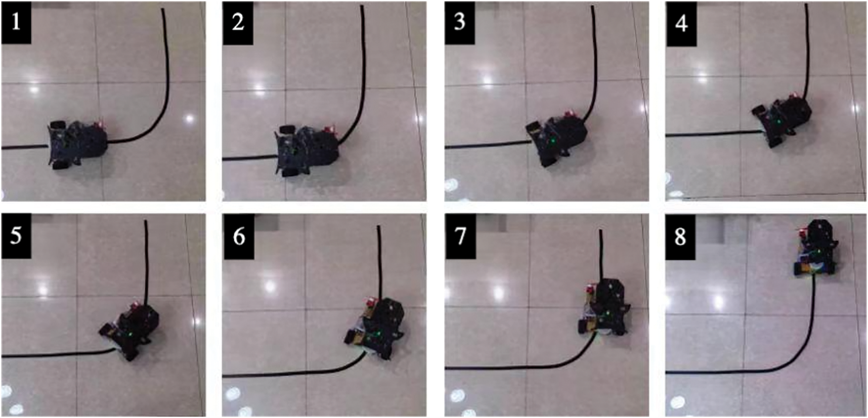
Figure 19: Curve experiment process

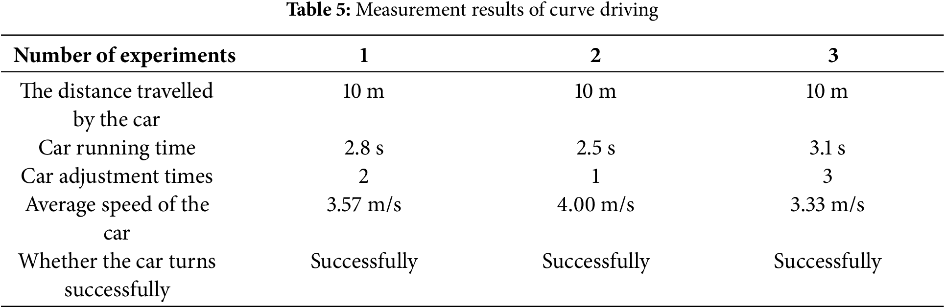
With the car speed set to 5 m/s, the results of multiple measurements are presented in Table 5. As shown in the table, during the curve driving experiment conducted several times, the car consistently followed the curve of the black line with precision in each trial, maintaining a speed of approximately 3.63 m/s.

5.2 Detection Experiment under Obstacles

In the actual movement of the car, the existence of obstacles should be considered. The ultrasonic ranging module on the front of the car can complete accurate obstacle avoidance experiments. The ultrasonic module can emit ultrasonic waves and calculate the time of ultrasonic wave return. The car’s distance to the obstacle can be calculated using the following formula. This section was divided into two different experimental works: one was the obstacle static experiment, and the other was the obstacle moving experiment.

(1) Obstacle static experiment

In the static obstacle experiment, static obstacles were randomly positioned along the path. If an obstacle was detected during the car’s movement, the car initiated a left rotation to assess potential barriers on the left side. If an obstacle was detected on the left, the car performed a significant right rotation until no obstacles were detected on either side. Subsequently, the car proceeded forward for a certain distance before rotating in the opposite direction. If no obstacles were detected, the car continued moving straight until it detected the black line, which adjusted its position accordingly. Eventually, the car returned to following the black line.

The static obstacle avoidance driving experiment of the test car is shown in Fig. 20. The car conducted the obstacle avoidance experiment when there was a static obstacle.

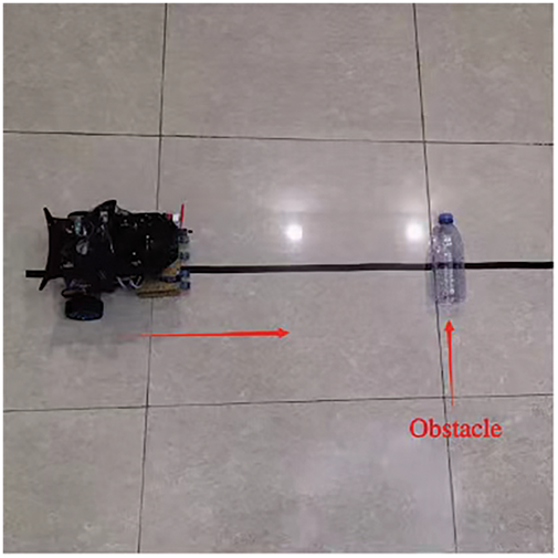
Figure 20: Schematic diagram of static obstacle experiment

Fig. 21-1 marked the starting point of the car’s movement. As the car progressed to the position depicted in Fig. 21-2, an obstacle was detected ahead. Subsequently, the car executed a slight left rotation to evade the obstacle. Once the obstacle was circumvented, the car proceeded to the position indicated in Fig. 21-4 and performed a slight rotation in the opposite direction. To continue its path, no obstacles were detected in Fig. 21-5, prompting the car to drive straight until it detected the presence of the black line, as shown in Fig. 21-6.

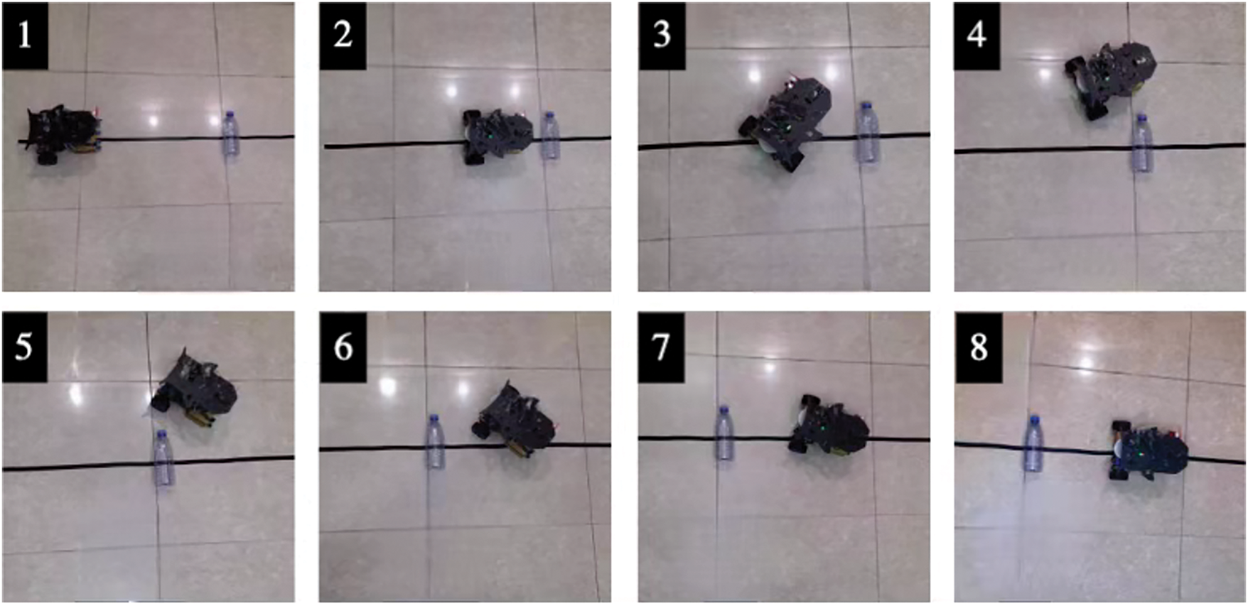
Figure 21: Static obstacle experiment process

Upon detecting the black line, the car adjusted its position accordingly, as depicted in Fig. 21-7, and ultimately returned to the black line as illustrated in Fig. 21-8. This series of manoeuvre allowed the car to navigate around obstacles and complete its path while staying within the designated route. Under the premise that the speed of the car was set to 5 m/s, the measurement results of obstacles placed at different positions are shown in Table 6.

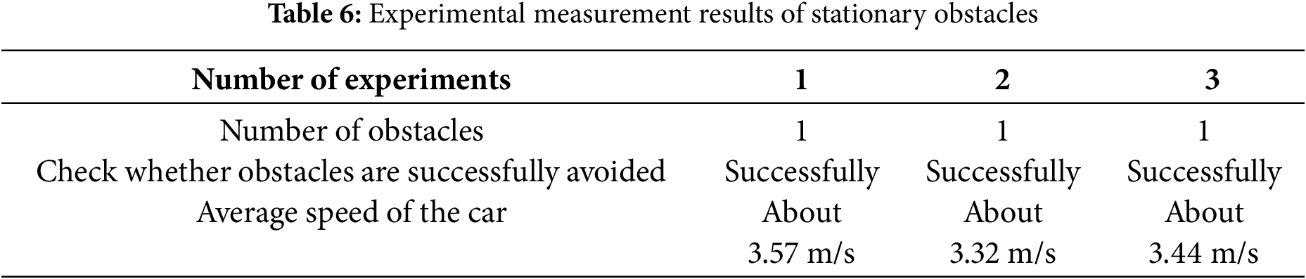
As shown in Table 6, in the experiment of placing obstacles in different positions many times, the car accurately and successfully avoided obstacles, and the speed was always maintained at about 3.44 m/s.

(2) Obstacle movement experiment

In real life, most obstacles were not stationary, and moving obstacles were also factors to test the performance of the car, so this section conducted the obstacle-moving experiment.

The obstacle movement experiment randomly placed moving obstacles on the path. When the car moved forward and detected an obstacle, the car rotated to the left to determine whether there was an obstacle in front of it. If there was no obstacle, the car moved according to the static experiment of the obstacle. If the obstacle moved to the path of the car, the car rotated in the opposite direction to determine whether it bypassed the obstacle and finally returned to the black line.

The obstacle avoidance driving experiment of the test car is shown in Fig. 22. The car conducted the obstacle avoidance experiment when there was a moving obstacle. When the car began to move, gave the obstacle an upward thrust, and observed the movement of the car.

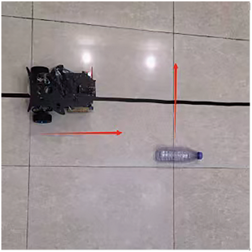
Figure 22: Schematic diagram of moving obstacle experiment

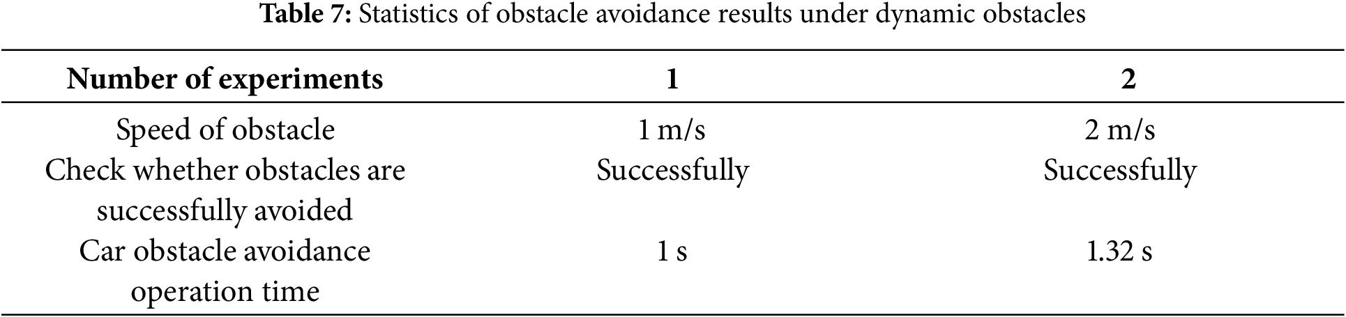
As depicted in Fig. 23-1, the car initiated movement from its starting point while the obstacle moved vertically toward the car’s direction. Upon reaching the position illustrated in Fig. 23-3, the car detected the moving obstacle and steered to the left. Subsequently, in Fig. 23-4, the car detected the obstacle again and adjusted its course to the right, as depicted in Fig. 23-5. This adjustment continued until no obstacle was detected, allowing the car to manoeuvred until it reached the black line, thereby completing the obstacle avoidance task. Under the premise that the speed of the car is set at 5 m/s, the test results of the car avoiding obstacles under different initial speeds of moving obstacles are shown in Table 7. As demonstrated by the data in Table 7, the car consistently avoided obstacles accurately and swiftly, even when faced with moving obstacles at varying speeds.

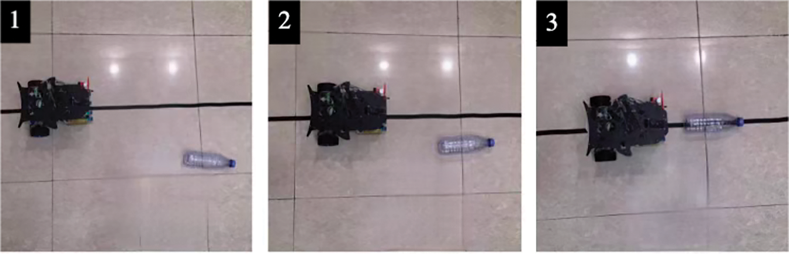
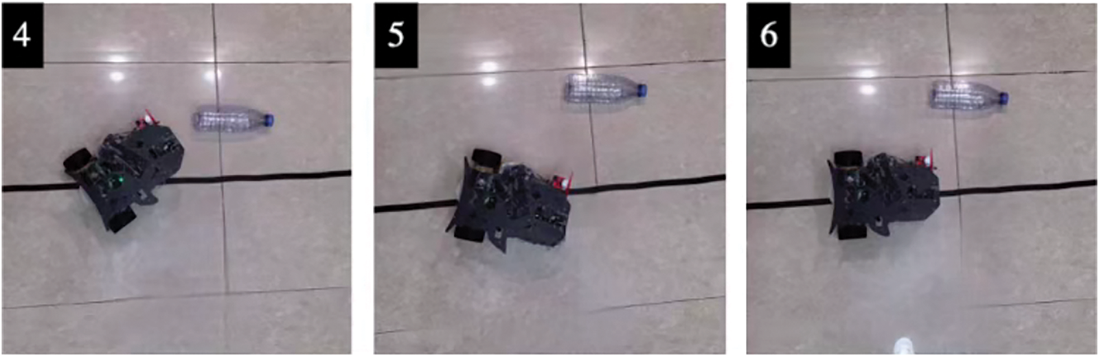
Figure 23: Experimental process of moving obstacles

6  Conclusion

This paper integrated PID design based on the BP neural network with intelligent car systems, showcasing their remarkable control capabilities in navigating complex systems, dynamic environments, and time-varying conditions. In obstacle experiments, the smart car promptly and accurately detected stationary or moving obstacles, made corresponding decisions to avoid collisions, and successfully returned to the established route, demonstrating the high real-time performance and robustness of the intelligent car designed with BP neural network PID.

However, this study has some limitations. We conducted experiments solely in indoor environments under sufficient lighting conditions, limiting the comprehensiveness of our findings. To more fully evaluate the performance of intelligent vehicles based on BP neural network PID design, future studies will focus on conducting experiments in more complex and harsh outdoor environments, particularly in dark conditions. By experimenting in diverse situations, we aim to understand smart car systems’ performance better and enhance their adaptability and practicality.

Therefore, future work will focus on optimizing the system for real-time performance under diverse environmental conditions, ensuring the system’s robustness and readiness for broader deployment. By addressing these challenges, the research lays a solid foundation for the development of intelligent vehicle systems capable of operating in real-world scenarios with high reliability and efficiency.

Acknowledgement: The authors would like to express our sincere gratitude to all the editors and anonymous reviewers for their valuable comments and constructive suggestions.

Funding Statement: This research was supported by the National Key Research and Development Program of China (No. 2023YFF0715103)—financial support, National Natural Science Foundation of China (Grant Nos. 62306237 and 62006191)—financial support, Key Research and Development Program of Shaanxi (Nos. 2024GX-YBXM-149 and 2021ZDLGY15-04)—financial support, Northwest University Graduate Innovation Project (No. CX2023194)—financial support, Natural Science Foundation of Shaanxi (No. 2023-JC-QN-0750)—financial support.

Author Contributions: Liang Zhou: Writing—original draft, Methodology, Software, Hardware, Validation; Qiyao Hu: Conceptualization, Methodology, Writing—review and editing, Formal analysis; Xianlin Peng: Preparation, Resources; Qianlong Liu: Validation. All authors reviewed the results and approved the final version of the manuscript.

Availability of Data and Materials: Not applicable.

Ethics Approval: Not applicable.

Conflicts of Interest: The authors declared no conflicts of interest to report regarding the present study.

References

1. Chougule A, Chamola V, Sam A, Yu FR, Sikdar B. A comprehensive review on limitations of autonomous driving and its impact on accidents and collisions. IEEE Open J Veh Technol. 2023;5:142–61. doi:10.1109/OJVT.2023.3335180. [Google Scholar] [CrossRef]

2. Patino HD, Liu D. Neural network-based model reference adaptive control system. IEEE Trans Syst Man Cybern Part B Cybern. 2000;30(1):198–204. doi:10.1109/3477.826961. [Google Scholar] [PubMed] [CrossRef]

3. Holkar K, Wagh K, Waghmare L. An overview of model predictive control. Int J Control Autom. 2010;3(4):47–63. [Google Scholar]

4. Berenji HR. Fuzzy logic controllers. In: An introduction to fuzzy logic applications in intelligent systems. Boston, MA, USA: Springer; 1992. p. 69–96. [Google Scholar]

5. Liu J, Lian Z, Shi J, Dong L, Sun C. Intermittent fixed-time fuzzy consensus of nonlinear multiagent systems with unknown control directions and event-based communication. IEEE Trans Fuzzy Syst. 2024;32(12):6917–28. doi:10.1109/TFUZZ.2024.3468022. [Google Scholar] [CrossRef]

6. Abdelwanis MI, El-Sousy FFM, Ali MM. A fuzzy-based proportional-integral–derivative with space-vector control and direct thrust control for a linear induction motor. Electronics. 2023;12(24):4955. doi:10.3390/electronics12244955. [Google Scholar] [CrossRef]

7. Ghamari SM, Khavari F, Mollaee H. Lyapunov-based adaptive PID controller design for buck converter. Soft Comput. 2023;27(9):5741–50. doi:10.1007/s00500-022-07797-z. [Google Scholar] [CrossRef]

8. Hanna YF, Khater AA, El-Nagar AM, El-Bardini M. Polynomial recurrent neural network-based adaptive PID controller with stable learning algorithm. Neural Process Lett. 2023;55(3):2885–910. doi:10.1007/s11063-022-10989-1. [Google Scholar] [CrossRef]

9. Saleem O, Ahmad KR, Iqbal J. Fuzzy-augmented model reference adaptive PID control law design for robust voltage regulation in DC-DC buck converters. Mathematics. 2024;12(12):1893. doi:10.3390/math12121893. [Google Scholar] [CrossRef]

10. Vanchinathan K, Selvaganesan N. Adaptive fractional order PID controller tuning for brushless DC motor using Artificial Bee Colony algorithm. Results Contr Optim. 2021;4:100032. doi:10.1016/j.rico.2021.100032. [Google Scholar] [CrossRef]

11. Li W, Qin K, Li G, Shi M, Zhang X. Robust bipartite tracking consensus of multi-agent systems via neural network combined with extended high-gain observer. ISA Trans. 2023;136:31–45. doi:10.1016/j.isatra.2022.10.015. [Google Scholar] [PubMed] [CrossRef]

12. Hanna YF, Khater AA, El-Bardini M, El-Nagar AM. Real time adaptive PID controller based on quantum neural network for nonlinear systems. Eng Appl Artif Intell. 2023;126:106952. doi:10.1016/j.engappai.2023.106952. [Google Scholar] [CrossRef]

13. Liu H, Yu Q, Wu Q. PID control model based on back propagation neural network optimized by adversarial learning-based grey wolf optimization. Appl Sci. 2023;13(8):4767. doi:10.3390/app13084767. [Google Scholar] [CrossRef]

14. Li J, Cheng JH, Shi JY, Huang F. Brief introduction of back propagation (BP) neural network algorithm and its improvement. In: Advances in computer science and information engineering. Berlin/Heidelberg: Springer; 2012. p. 553–8. doi :10.1007/978-3-642-30223-7_87. [Google Scholar] [CrossRef]

15. Dalboni M, Mangoni D, Lusignani D, Soldati A. Lightweight dynamic vehicle models oriented to vehicle electrification. Int J Veh Perform. 2019;5(1):40. doi:10.1504/IJVP.2019.097097. [Google Scholar] [PubMed] [CrossRef]

16. Brancaleoni PP, Corti E, Ravaglioli V, Moro D, Silvagni G. Innovative torque-based control strategy for hydrogen internal combustion engine. Int J Hydrog Energy. 2024;73:203–20. doi:10.1016/j.ijhydene.2024.05.481. [Google Scholar] [CrossRef]

17. Hong Y, Li J, Wang W, Chen J, Wei R. A driving assist system for path tracking via active rear-wheel steering. In: 2021 33rd Chinese Control and Decision Conference (CCDC); 2021; Kunming, China. p. 1104–9. doi:10.1109/CCDC52312.2021.9602571 [Google Scholar] [CrossRef]

18. Dandiwala A, Chakraborty B, Chakravarty D, Sindha J. Vehicle dynamics and active rollover stability control of an electric narrow three-wheeled vehicle: A review and concern towards improvement. Veh Syst Dyn. 2023;61(2):399–422. doi:10.1080/00423114.2022.2046810. [Google Scholar] [CrossRef]

19. Sindha J, Chakraborty B, Chakravarty D. Automatic stability control of three-wheeler vehicles-recent developments and concerns towards a sustainable technology. Proc Inst Mech Eng Part D J Automob Eng. 2018;232(3):418–34. doi:10.1177/0954407017701285. [Google Scholar] [CrossRef]

20. Ataei M, Khajepour A, Jeon S. Development of a novel general reconfigurable vehicle dynamics model. Mech Mach Theory. 2021;156:104147. doi:10.1016/j.mechmachtheory.2020.104147. [Google Scholar] [CrossRef]

21. Defazio A, Konstantin M. Learning-rate-free learning by d-adaptation. In: International Conference on Machine Learning. PMLR; 2023. [Google Scholar]

22. Liao W. Real time bearing fault diagnosis based on convolutional neural network and STM32 microcontroller. arXiv:2304.09100. 2023. [Google Scholar]

23. Brown J, Smith A. Advanced serial communication with FT232RL USB to TTL adapter. Int J Embed Syst. 2020;45(2):123–30. [Google Scholar]

24. Lee K, Kim H. Power optimization techniques for OLED displays in wearable devices. J Display Technol. 2019;15(5):256–62. [Google Scholar]

25. Zhang L, Wang Y. IoT-based environmental monitoring with DHT11 sensor. Sensor Actuat A: Phys. 2021;304:111940. [Google Scholar]

26. Thompson R, Johnson M. Efficient power management with LM2596 voltage regulators. J Power Electron. 2020;17(6):458–65. [Google Scholar]

27. Fuada S, Hendriyana H. UPISmartHome V.2.0—a consumer product of smart home system with an ESP8266 as the basis. J Commun. 2022;17(7):541–52. doi:10.12720/jcm.17.7.541-552. [Google Scholar] [CrossRef]

28. Pei R, Cao Y. Design of multi-channel temperature acquisition system based on STM32. J Artif Intell Pract. 2023;6(1):41–7. doi:10.23977/jaip.2023.060106. [Google Scholar] [CrossRef]

29. Liu H, Chen G. An improved line following algorithm for autonomous mobile robots using infrared sensors. IEEE Access. 2022;10:38729–39. [Google Scholar]

30. Lee J, Kim J, Park S. Development of a fire detection system using sensor data and deep learning algorithms. Sensors. 2021;21(5):1623. [Google Scholar]

31. Chen Y, Wang J. Real-time ultrasonic sensor-based obstacle avoidance system for mobile robots. Robot Auton Syst. 2021;140:103783. [Google Scholar]

32. Ome N, Rao GS. Internet of Things (IoT) based sensors to cloud system using ESP8266 and Arduino Due. Int J Adv Res Comput Commun. 2016;5(10):337–43. [Google Scholar]

33. Hatton M. IoT in 2024: trends and predictions. USA: IoT For All; 2024. [Google Scholar]