Deterministic Convergence Analysis for GRU Networks via Smoothing Regularization

1  Introduction

Recurrent Neural Networks (RNN) have emerged as a powerful class of neural networks, particularly adept at modeling sequential data due to their ability to retain and utilize temporal dependencies [1]. These networks have demonstrated remarkable success across various domains, including natural language processing, speech recognition, and time-series forecasting [2]. However, the application of RNN is not without challenges. One of the primary issues is the vanishing and exploding gradient problem, which can significantly hinder the training of deep RNN [3,4]. To address this, several variants of RNN have been proposed, such as Long Short-Term Memory Networks (LSTM) and Gated Recurrent Units (GRU) [5,6]. These architectures incorporate gating mechanisms to selectively retain or forget information, effectively mitigating gradient-related issues and improving performance [7]. LSTM, for instance, uses a combination of input, forget, and output gates to control the flow of information, allowing the network to retain relevant information over extended sequences [8]. Similarly, GRU simplifies the gating mechanism while maintaining comparable performance, making them computationally more efficient [9].

Despite the advancements in RNN architectures, the issue of overfitting remains a significant challenge, particularly when dealing with limited or noisy data [10]. Overfitting occurs when a model learns to memorize the training data instead of generalizing to unseen samples, leading to poor performance on test data [11,12]. Regularization techniques have been introduced to address this, aiming to improve the generalization ability of neural networks by controlling their complexity. Common regularization methods, such as L2 regularization and dropout, have shown efficacy in various settings [13–15].

L2 regularization penalizes large weights by adding their squared magnitude to the loss function, thereby encouraging simpler models [16,17]. Dropout, on the other hand, randomly deactivates neurons during training, preventing the network from relying too heavily on specific features [18–20]. L1 regularization can suppress weight growth to enhance model performance and increase parameter sparsity to improve computational efficiency [21–23]. Building on these methods, researchers have analyzed the theoretical properties of regularized networks. Zhang et al. [24] investigate a penalized batch backpropagation algorithm for training feedforward neural networks. They establish the boundedness, as well as the weak and strong convergence properties of the algorithm, using mathematical methods. Similarly, Wang et al. [25] prove the boundedness of backpropagation neural networks (BPNN) with L2 regularization and provide convergence results based on this. Kang et al. [26] incorporate an adaptive momentum term into the iterative error function when training the group lasso-regularized Sigma Pi Sigma neural network, thus boosting the algorithm’s convergence speed and reducing the model’s training time. Yu et al. [27] optimize a generalized learning system using L1/2 regularization, further examining its theoretical properties and performance. However, there are significant difficulties in the theoretical analysis of L1 regularization [28]. The L1 regularization term is often written as (1):

Ω(w)=‖w‖1=∑i|wi|(1)

where ‖⋅‖1 represents 1-norm. Obviously, the L1 regularization term lacks a derivative at the origin [29,30]. Therefore, it is necessary to introduce smoothing approximation functions to solve the non-differentiability problem of L1 regularization [31].

In this research, we propose the use of GRU networks with smoothing L1 regularization to address the aforementioned challenges. Unlike traditional L1 regularization, which can introduce non-differentiable points, the smoothed variant ensures a more stable optimization process, making it better suited for modern neural network architectures.

This research primarily focuses on analyzing the monotonicity, weak convergence, and strong convergence properties of GRU networks with smoothing L1 regularization (referred to as SL1-GRU), including theoretical proofs and simulation experiments. This paper makes the following contributions:

(1) The smoothing L1 regularization is integrated into the network, effectively overcoming the oscillation phenomenon caused by traditional L1 regularization. At the same time, the redundant weight values in the network are trimmed, further optimizing the network structure and improving its sparsity.

(2) Under given conditions and assumptions, the monotonicity, weak convergence, and strong convergence of SL1-GRU are theoretically demonstrated. The network’s error function decreases monotonically with the increasing number of iterations. As iterations approach infinity, weak convergence is demonstrated by the error function’s gradient approaching zero. Strong convergence means network weights can converge to a fixed point under defined conditions.

(3) The theoretical results are validated through experiments on approximation, classification, and regression tasks. The experimental results show that GRU networks with smoothing L1 regularization achieve excellent performance in solving various machine learning problems, with high sparsity generated during the network weights optimization process, which is conducive to optimizing the network structure, reducing the possibility of overfitting and improving the generalization ability of the network.

The rest of this paper is structured as follows: Section 2 explores the GRU network structure and the parameter iteration mechanism after introducing smoothing L1 regularization. Section 3 discusses the principal theoretical achievements. Section 4 confirms the theoretical findings and the practical performance of SL1-GRU through simulation experiments. Lastly, Section 5 encapsulates the research content and discusses possible directions for future investigations. The detailed proofs of theorems and corollaries are included in the Appendix A.

2  GRU Based on Regularization Method

2.1 Network Structure of GRU

As a streamlined variant of LSTM, GRU features just two gate mechanisms: an update gate and a reset gate [32]. The internal configuration of GRU, shown in Fig. 1, together with the standard forward propagation equations, is detailed below:

zt=σ(Wz[ht−1,xt]+bz)(2)

rt=σ(Wr[ht−1,xt]+br)(3)

h~t=tanh⁡(Wh~[rt∘ht−1,xt]+bh~)(4)

ht=zt∘h~t+(1−zt)∘ht−1(5)

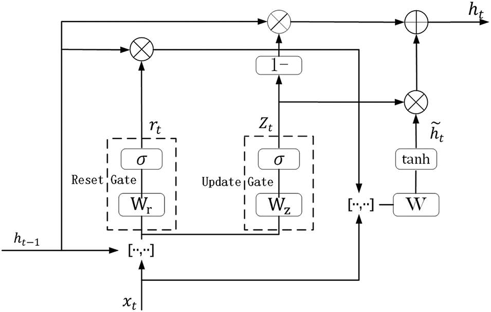
Figure 1: Structure of GRU

The following are the explanations for the related symbols:

•   The symbol ∘ stands for the Hadamard product, which refers to element-wise multiplication.

•   [⋅,⋅] denotes the concatenation of two vectors into a longer vector.

•   xt denotes the input to the network at time t.

•   zt and rt correspond to the update outputs and reset gate outputs at time t, respectively.

•   At time t, h~t denotes the candidate output, while ht represents the output of hidden layer.

•   The symbols Wr, Wz, and Wh~ respectively signify the weight matrices associated with the reset gate, the update gate, and the candidate output.

•   σ represents the sigmoid function, a nonlinear activation mapping real-valued inputs to the range (0, 1). Similarly, tanh is a nonlinear function that maps inputs to the range (−1, 1).

•   br, bz, and bh~ correspond to the biases for the respective weight matrices.

In (2), Wz denotes the weight matrix associated with the update gate. In fact, Wz is formed by concatenating two matrices: Wz,h, which corresponds to the input vector ht−1, Wz,x, which corresponds to the input vector. Therefore, Eq. (2) can be written as:

[Wz][ht−1xt]=[Wz,hWz,x][ht−1xt]=Wz,hht−1+Wz,xxt(6)

Obviously, the weight matrix in other Eqs. (3)–(5) can be also rewritten in the same form as (6). For the convenience of subsequent analysis, we set the biases br, bz, and bh~ to 0 and get new expressions as follows:

zt=σ(Wz,h⋅ht−1+Wz,x⋅xt)(7)

rt=σ(Wr,h⋅ht−1+Wr,x⋅xt)(8)

h~t=tanh⁡(Wh~⋅(rt∘ht−1)+Wh~⋅xt)(9)

ht=(1−zt)∘ht−1+zt∘h~t(10)

If {xn,Tn}n=1N⊂RN×RN as the given set of the training samples, where the xn represent the n-th input sample and the Tn is the label, respectively. Let ytn=σ(wout⋅htn)∈R be the actual output for each input Xn, and yt0=wout ⋅ht. Thereby, the error function is defined by the following formula:

E~(W)=12N∑n=1N(ytn−Tn)2=12N∑n=1N(σ(wout ⋅htn)−Tn)2=1N∑n=1Nσn(wout ⋅htn)(11)

where σn(r)=12(σ(r)−Tn)2,r∈R,1≤n≤N.

2.2 Gradient Learning Method with Smoothing L1 Regularization for GRU

The standard approach to achieve L1 regularization entails incorporating a penalty term within the error function, expressed as:

E(W)=E~(W)+λ‖wout ‖1(12)

This can be written as:

E(W)=∑n=1Nσn(wout ⋅htn)+λ‖wout ‖1(13)

where λ>0 is the penalty parameter, while ||⋅||1 indicates L1-norm.

However, there is no derivative of the L1 regularization term at the origin [33,34]. To tackle the non-differentiable problem of the L1 regularization term, a smoothing approximation function is introduced. Smoothing approximation is essentially the use of continuous differentiable functions instead of absolute value functions. In this paper, a quadratic form smoothing approximation function is used, which means:

h(x)={|x|,|x|≥α|x|22α+α2,|x|<α(14)

The smoothing coefficient α is a constant greater than zero. Fig. 2 illustrates the effect of α on the degree of approximation. It is easy to see that when the smoothing coefficient α tends to zero, the approximation function increasingly resembles the absolute function. Therefore, in practical applications, the smaller the smoothing coefficient, the closer the actual effect of the regularization term is to the L1 regularization method.

Figure 2: Influence of smoothing coefficient on fitting degree

By incorporating a smooth approximation function into the error propagation mechanism of L1 regularized GRU, the issue of non-differentiability at the origin is overcome, providing a basis for a rigorous analysis of the error function’s monotonicity. Specifically, the error function expression of the smoothed SL1-GRU model is derived as follows by replacing the L1 regularization term with the smoothed approximation function L1(Wout):

E=∑n=1Nσn(Wout ⋅htn)+λL1(Wout ),λ>0(15)

The element L1(Wouti,j) is positioned in the i-th row and j-th column of the matrix L1(Wout). Specifically, L1(Wouti,j) is defined as follows:

L1(Wouti,j)={|Wouti,j|,if |Wouti,j|≥α|Wouti,j|22α+α2,if |Wouti,j|<α(16)

here, α is a given bounded constant.

The optimization algorithm, Stochastic Gradient Descent (SGD), is frequently used to train GRU. To achieve the fastest reduction of the error function E, the direction of weight changes should be the same as the negative gradient of E in the weight matrix. The learning rate, symbolized by η, is a scalar hyperparameter that determines the step increment for each iteration in the optimization algorithm. ∇WE represents the partial derivative of the error function E with respect to the weight W. If Wk and Wk+1 denote the weight matrices for the k-th and (k+1)-th iterations, respectively, and ΔWk represents the change in the weight matrix from Wk to Wk+1. The weight update rule for the SGD algorithm is defined as:

Wk+1=Wk+ΔWk=Wk−η∇WE(17)

This equation indicates that during each iteration, SL1-GRU updates the weights by deducting the result of multiplying the learning rate η by the gradient of the error function with respect to the weights from the current weight matrix Wk, causing the weights to change in a direction that reduces the error function. By iteratively applying this rule, the weights are adjusted to minimize the error.

Define δh,tk as the partial derivative of E over htk, and it is given by:

δh,tk=∂E∂htk(18)

Similarly, define:

δz,tk=∂E∂ztk∘ztk∘(1−ztk)=δh,tk∘(h~tk−ht−1k)∘ztk∘(1−ztk)(19)

δr,tk=∂E∂rtk∘rtk∘(1−rtk)=ht−1k∘[(δh,tk∘ztk∘(1−(h~tk)2t)Whk]∘rtk∘(1−rtk)(20)

δh~,tk=∂E∂h~tk∘(1−(h~tk)2)=δh,tk∘ztk∘(1−(h~tk)2)(21)

For each weight matrix, the partial derivatives of E are as follows:

∇Wz,hkE=∂E∂Wz,hk=∑i=1tδz,ikhi−1k,(22)

∇Wz,xkE=∂E∂Wz,xk=∑i=1tδz,ikxik,(23)

∇Wr,hkE=∂E∂Wr,hk=∑i=1tδr,ikhi−1k,(24)

∇Wr,xkE=∂E∂Wrx=∑i=1tδr,ikxik,(25)

∇Wh~,rkE=∂E∂Whk=∑i=1tδik(rik∘hi−1k),(26)

∇Wh~,xkE=∂E∂Wxk=∑i=1tδikxik,(27)

For the output weight matrix Wout, the partial derivative of E specifically is:

∂E∂Woutk=∑n=1Nσn′(Woutk⋅htk,n)ΔWoutk⋅htk,n+λ∂L1(Wout)∂Wout(28)

where λ>0.

According to (17) and (22) to (28), the weights are updated iteratively by:

Wz,hk+1=Wz,hk+ΔWz,hk=Wz,hk−η∂E∂Wz,hk(29)

Wz,xk+1=Wz,xk+ΔWz,xk=Wz,xk−η∂E∂Wz,xk(30)

Wr,hk+1=Wr,hk+ΔWr,hk=Wr,hk−η∂E∂Wr,hk(31)

Wr,xk+1=Wr,xk+ΔWr,xk=Wr,xk−η∂E∂Wr,xk(32)

Wh~,rk+1=Wh~,rk+ΔWh~,rk=Wh~,rk−η∂E∂Wh~,rk(33)

Wh~,xk+1=Wh~,xk+ΔWh~,xk=Wh~,xk−η∂E∂Wh~,xk(34)

Woutk+1=Woutk+ΔWoutk=Woutk−η∂E∂Woutk(35)

Based on the above analysis, the SL1GRU algorithm flow is presented in Algorithm 1.

3  Convergence Analysis

This section presents the theoretical findings of GRU networks with smoothing L1 regularization, with detailed proofs available in Appendix A. To ensure the validity and correctness of the proposed statements and conclusions, the following mild assumptions are made:

(A1) For r∈R,|σ(r)|,|σ′(r)|,|σ′′(r)|,|tanh⁡(r)|, |tanh′⁡(r)|, and |tan′′⁡(r)| are uniformly bounded.

(A2) λ and η are chosen to meet the conditions of 0<η<2(1+D4)λC+4D4+2D5, where D4 and D5 are constants defined in below.

(A3) There exists a bounded region Ω⊂Rn such that {wout k}k=0∞⊂Ω.

(A4) A compact set ϕ0 exists where Wk∈ϕ0, and the set ϕ1={W∈ϕ0:∂E∂W=0} includes only a finite number of points.

Our main results are as follows:

Theorem 1. Monotonicity

Assume the error function E(W) is given as in Eq. (15). Consider the sequence of weights Wk produced by the iterative algorithm detailed in Eq. (17), with an arbitrary initial weight W0. Under the assumptions (A1)−(A3), the following monotonicity property holds:

E(Wk+1)≤E(Wk),for k=0,1,2,….(36)

Theorem 2. Weak Convergence

Assuming that conditions (A1)–(A3) hold, then the weight sequence Wk generated by (17) is weak convergent, as evidenced by the following equation:

limk→+∞‖∂E∂Wk‖=0(37)

Theorem 3. Strong Convergence

Furthermore, if assumption (A4) also holds, the subsequent strong convergence outcome can be derived:

limk→∞(Wk)=W∗(38)

where W∗∈ϕ0.

For clarity and convenience, certain notations will be introduced for future reference.

D0=max1≤n≤N{‖xtn‖,‖ht−1n‖}D1=max{supr∈R|σ(r)|,supr∈R|σ′(r)|,supr∈R|σ′′(r)|,supr∈R,1≤n≤N|σn′(r)|,supr∈R|tanh⁡(r)|,supr∈R|tanh′⁡(r)|,supr∈R|tanh′′⁡(r)|,supr∈R,1≤n≤N|tanhn′⁡(r)|},D2=max{‖woutk‖}.(39)

4  Experimental Results and Analysis

The experiment is divided into three distinct parts. The initial part involves an analysis of theoretical outcomes through the approximation of function. Subsequently, the generalization capability and sparsity of the model are evaluated using regression and classification datasets from the UCI Machine Learning Repository.

4.1 Function Approximation

To demonstrate the generalization capabilities of SL1-GRU, we approximate a one-dimensional function f(x) and a two-dimensional function q(x,y) in this section. The mathematical expressions of these functions are as follows:

Nonlinear oscillatory function:

f(x)=8+2e1−x2cos⁡(2πx),x∈[−0.5,3.5](40)

The peaks function, commonly used in numerical experiments, defined as:

q(x,y)=3(1−x)2e−x2−(y+1)2−10(x5−x3−y5)e−x2−y2−13e−(x+1)2−y2,x,y∈[−2.5,2.5](41)

For the nonlinear oscillatory function (40), 100 points are uniformly distributed in the interval [−0.5,3.5] and denoted as xi for i=1,2,…,100, serving as inputs. The corresponding outputs are given by f(xi)+ϵi, where ϵi∼N(0,0.01). For the peaks function (41), a two-dimensional grid is generated with x,y uniformly sampled within [−2.5,2.5], resulting in 100 sample points. The outputs are perturbed by Gaussian noise ϵi,j∼N(0,0.01), yielding q(xi,yj)+ϵi,j. The network weights of six models (RNN, LSTM, GRU, L1-GRU, L2-GRU, SL1-GRU) are initialized randomly in [−0.5,0.5], with the learning rate η set to 0.001. Regularization coefficients for L1-GRU, L2-GRU and SL1-GRU are λ=0.0005, while the smoothing parameter for SL1-GRU is α=0.01.

Fig. 3a shows the approximation performance of RNN, LSTM, GRU, L1-GRU, L2-GRU, and SL1-GRU for the nonlinear target function f(x) in [0.5,3.5]. Regularized models (L1-GRU, L2-GRU, SL1-GRU) align more closely with the actual curve, with SL1-GRU achieving the best accuracy in oscillatory regions, highlighting its robustness in capturing nonlinear dynamics. Fig. 3b illustrates the sparsity evolution over training iterations. L1-GRU and SL1-GRU achieve significantly higher sparsity, stabilizing around 0.8 after 2000 iterations, while GRU and LSTM show lower sparsity, reflecting greater parameter complexity. These results demonstrate the effectiveness of regularization in promoting model sparsity.

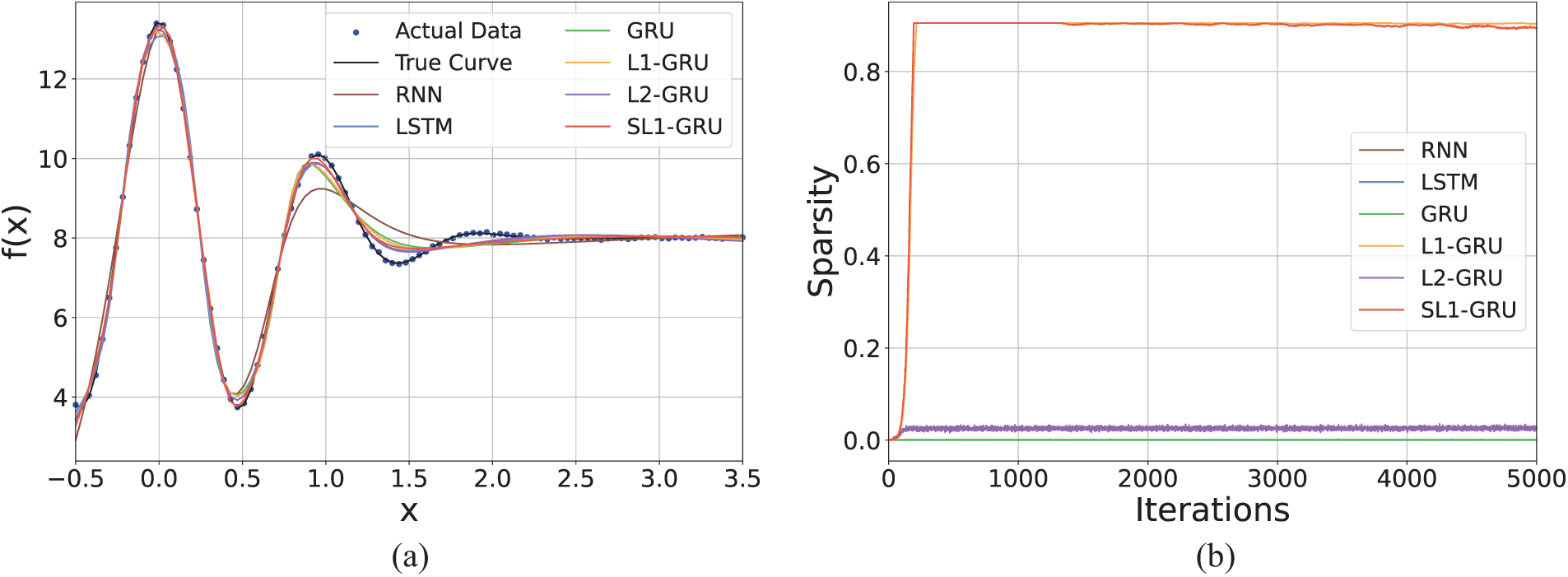
Figure 3: Approximation perfomance for one-dimensional function (a) results of approximation (b) sparsity of models

Similarly, we approximate the two-dimensional function using the same approaches, with the approximation results of SL1-GRU presented in Fig. 4. The results highlight SL1-GRU’s ability to effectively capture global trends and local variations.

Figure 4: Approximation result of SL1-GRU for two-dimensional function (a) two-dimensional function (b) approximation function

4.2 Classification Problem

This part presents an evaluation and comparison of the classification efficacy for RNN, LSTM, GRU, L1-GRU, L2-GRU, and SL1-GRU. Table 1 is a summary of the dataset utilized in the simulation experiment. The network weights are randomly initialized in [−0.5,0.5]. Each network is set up with a hidden layer of 32 nodes. The dataset’s features determine the input layer’s node count, while the number of output layer nodes equals the count of classes.

As shown in Fig. 5, we use grid search to explore the hyperparameter space by testing combinations of learning rate η, regularization factor λ, and smoothing coefficient α within predefined ranges. Each combination of these hyperparameters is evaluated using k-fold cross-validation to ensure robust and reliable performance metrics. The evaluation criterion is based on the test accuracy achieved by SL1-GRU, aiming to identify the parameter set that maximizes accuracy while maintaining generalization. It is determined that {α=0.01,λ=0.00005,η=0.005} constitutes the optimal parameter combination for the wine dataset, achieving the highest test accuracy for SL1-GRU. This approach is similarly applied to other datasets, and the results, summarized in Table 2, highlight the effectiveness of grid search in identifying optimal hyperparameters.

Figure 5: Test accuracy of SL1-GRU on the wine dataset under different parameter combinations; α is regularization coefficient

Table 3 compares the training accuracy, test accuracy, sparsity, and training time of different models on the same dataset. These experimental results represent the average values obtained over 10 trials. Sparsity, defined as the ratio of elements in the neural network’s weight matrix that are less than 1×10−5 to the total number of elements in the weight matrix, is used as an indicator of network sparsity. Mathematically, it can be expressed as:

Sparsity=Num0Numn(42)

where the number of elements in the weight matrix that are less than 1×10−5 is denoted by Num0, and Numn represents the overall element count of the matrix. It can be observed in Table 3 that although the training accuracy of SL1-GRU may not be the highest, its test accuracy is consistently the best across all datasets, highlighting its excellent generalization ability. Moreover, both L1-GRU and SL1-GRU exhibit significantly higher sparsity compared to other models. Except for one dataset, SL1-GRU achieves the highest sparsity, demonstrating that the proposed method effectively enhances network sparsity. Additionally, benefiting from its superior sparsity, SL1-GRU requires the shortest training time, indicating that it significantly improves computational efficiency.

From Fig. 6, it can be observed that the loss function curve of SL1-GRU monotonically decreases and gradually stabilizes at zero as the number of iterations increases, which verifies Theorem 1. Meanwhile, in Fig. 6b, the gradient curve of SL1-GRU decreases the fastest, and as the number of iterations approaches infinity, its gradient also tends to zero, consistent with Theorem 2. Fig. 6c shows that the weight curves of L1-GRU and SL1-GRU do not grow indefinitely, indicating that both regularization methods effectively suppress weight growth. Among them, SL1-GRU is more effective in constraining network weights, stabilizing them around a constant value of approximately 140, aligning with Theorem 3.

Figure 6: The performance of RNN, LSTM, GRU, L1-GRU, L2-GRU and SL1-GRU on MNIST dataset; the shaded area presents the mean ± the standard deviation over 10 trials

4.3 Regression Problem

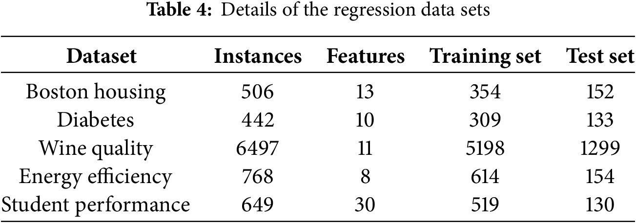
The performance of SL1-GRU in regression tasks is also considered. The dataset utilized in this part is detailed in Table 4. For RNN, LSTM, GRU, L1-GRU, L2-GRU, and SL1-GRU, the hidden layer is designed with 32 nodes. The nodes in both the input and output layers are configured based on the dataset’s features and labels, respectively. The learning rate is established at η=1×10−3, the regularization factor at λ=3×10−4, and the smoothing coefficient at α=0.01. The initial weight range is [−0.5,0.5] as in the previous part.

In the evaluation of regression models, the standard metric used is Mean Squared Error (MSE), which is calculated using the following formula:

MSE=1n∑i=1n(predi−truei)2,(43)

where pred1,pred2,…,predn indicate the predicted values, and the set of actual values is denoted by true1,true2,…,truen.

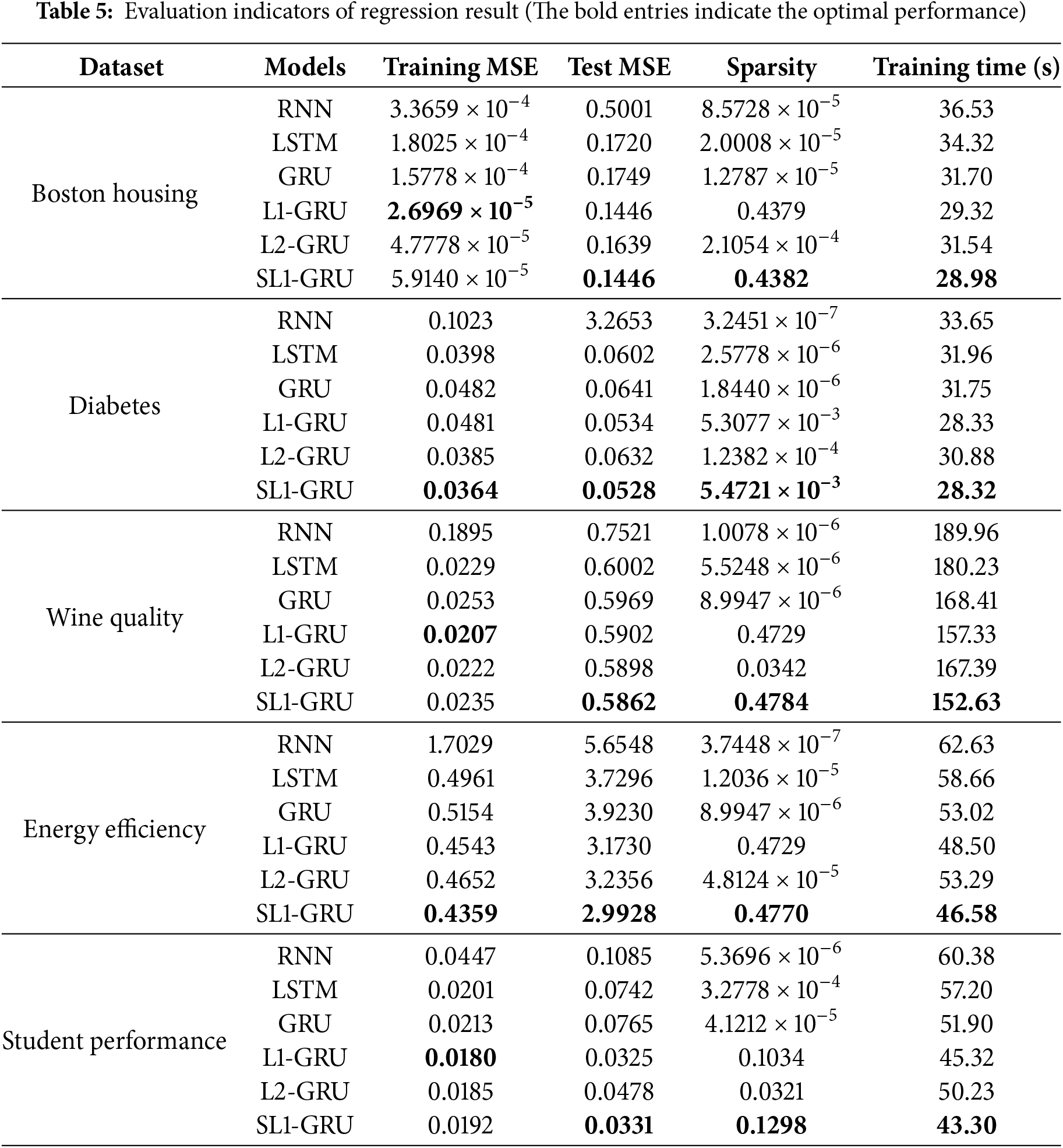
Table 5 shows that the Test MSE of SL1-GRU is consistently the smallest, indicating that it performs the best on the test set and has the strongest generalization ability. From the perspective of sparsity, the network weights of SL1-GRU remain the sparsest, which suggests that it eliminates unimportant parameters to enhance the computational efficiency of the model while maintaining its excellent performance.

5  Conclusions

This article proposes a GRU with smoothing L1 regularization to address the issue of non-differentiability at the origin inherent in traditional L1 regularization. This approach also aims to enhance the network sparsity and generalization capability. We theoretically demonstrate the monotonicity, weak convergence, and strong convergence of SL1-GRU in backpropagation algorithms and design simulation experiments to compare SL1-GRU with RNN, LSTM, GRU, L1-GRU, and L2-GRU. The simulation results align with the theoretical analysis, demonstrating that SL1-GRU effectively curbs excessive weight growth, reduces the risk of overfitting, and enhances the network’s generalization capability. In addition, SL1-GRU also performs well in handling classification and regression problems on real-world datasets, indicating its usability in practical problems. Future work will focus on conducting theoretical analysis under more relaxed assumptions. Furthermore, we will investigate whether dynamically adjusting the smoothing coefficients can further optimize model performance. For example, the smoothing coefficients could be adaptively adjusted based on gradient changes during training.

Acknowledgement: We would like to thank the editors and reviewers for their valuable work.

Funding Statement: This work was supported by the National Science Fund for Distinguished Young Scholarship (No. 62025602), National Natural Science Foundation of China (Nos. U22B2036, 11931015), the Fok Ying-Tong Education Foundation China (No. 171105), the Fundamental Research Funds for the Central Universities (No. G2024WD0151) and in part by the Tencent Foundation and XPLORER PRIZE.

Author Contributions: Qian Zhu: Conceptualization, Software, Writing—review & editing. Qian Kang: Data curation, Writing—review. Tao Xu: Conceptualization, Validation, Methodology. Dengxiu Yu: Methodology, Supervision, Validation. Zhen Wang: Supervision, Validation. All authors reviewed the results and approved the final version of the manuscript.

Availability of Data and Materials: The datasets used and/or analyzed during the current study are available from the corresponding author on reasonable request.

Ethics Approval: Not applicable.

Conflicts of Interest: The authors declare no conflicts of interest to report regarding the present study.

Appendix A

Detailed Proof: Lemma A1. The function f(x) is specified over a closed and bounded [a,b], with its derivative f′(x) being Lipschitz continuous, constant c>0. Then the following equationas holds:

f(x)≤f(x0)+f′(x0)(x−x0)+c2(x−x0)2,∀x0,x∈[a,b](A1)

Proof of Lemma A1. □

A new function is constructed as:

g(x)=f(x)−f(x0)−f′(x0)(x−x0)−c2(x−x0)2(A2)

where c denotes a positive constant.

Taking the derivative of x

g′(x)=f′(x)−f′(x0)−c(x−x0)(A3)

|f(x)−f′(x0)|≤c|x−x0|(A4)

{g′(x)≤0,x≥x0g′(x)≥0,x<x0(A5)

then,

g(x)≤g(x0)=0(A6)

Proof of Theorem 1. □

By (15), the errors at the k-th and (k+1)-th iterations are given as:

Ek+1=∑n=1Nσn(Woutk+1⋅htk+1,n)+λL1(Woutk+1)(A7)

Ek=∑n=1Nσn(Woutk⋅htk,n)+λL1(Woutk)(A8)

and the difference between them is:

Ek+1−Ek=∑n=1Nσn(Woutk+1⋅htk+1,n)+λL1(Woutk+1)−[∑n=1Nσn(Woutk⋅htk,n)+λL1(Woutk)]=∑n=1N[σn(Woutk+1⋅htk+1,n)−σn(Woutk⋅htk,n)]+λ[L1(Woutk+1)−L1(Woutk)]=∑n=1N[σ′n(Woutk⋅htk,n)(Woutk+1⋅htk+1,n−Woutk⋅htk,n)]+R1+λ[L1(Woutk+1)−L1(Woutk)]=∑n=1Nσ′n(Woutk⋅htk,n)ΔWoutk⋅htk,n+∑n=1Nσ′n(Woutk⋅htk,n)Woutk⋅Δhtk,n+∑n=1Nσ′n(Woutk⋅htk,n)ΔWoutk⋅Δhtk,n+R1+λ[L1(Woutk+1)−L1(Woutk)]=∑n=1Nσ′n(Woutk⋅htk,n)ΔWoutk⋅htk,n+λ[L1(Woutk+1)−L1(Woutk)]+∑n=1Nσ′n(Woutk⋅htk,n)Woutk⋅Δhtk,n+∑n=1Nσ′n(Woutk⋅htk,n)ΔWoutk⋅Δhtk,n+R1(A9)

where Lagrange remainder

R1=12∑n=1Nσ′′(sk,n)(Woutk+1htk+1,n−Woutkhtk,n)2(A10)

in the above equation, sk,n is a constant between Woutk+1htk+1,n and Woutkhtk,n.

To simplify, we use the following notation:

A1=∑n=1Nσ′n(Woutk⋅htk,n)ΔWoutk⋅htk,n+λ[L1(Woutk+1)−L1(Woutk)](A11)

A2=∑n=1Nσ′n(Woutk⋅htk,n)Woutk⋅Δhtk,n(A12)

A3=∑n=1Nσ′n(Woutk⋅htk,n)ΔWoutk⋅Δhtk,n(A13)

According to Lemma A1,

λ[L1(Woutk+1)−L1(Woutk)]≤λ[L1′(Woutk)[L1(Woutk+1)−L1(Woutk)]+c2[L1(Woutk+1)−L1(Woutk)]2]≤λL1′(Woutk)ΔL1(Woutk)+λc2[ΔL1(Woutk)]2(A14)

Using transition variables

Δhtk,n=htk+1,n−htk,n=[(1−ztk+1,n)∘ht−1n+ztk+1,n∘h~tk+1,n]−[(1−ztk,n)∘ht−1n+ztk,n∘h~tk,n]=ztk+1,n∘h~tk+1,n−ztk,n∘h~tk,n+(1−ztk+1,n)∘ht−1n−(1−ztk,n)∘ht−1n=(ztk+1,n−ztk,n)∘(h~tk+1,n−h~tk,n)+(ztk+1,n−ztk,n)∘h~tk,n+ztk,n∘(h~tk+1,n−h~tk,n)−(ztk+1,n−ztk,n)∘ht−1n=[σ(Wz,hk+1,n⋅ht−1n+Wz,xk+1,n⋅xtn)−σ(Wz,hk,n⋅ht−1n+Wz,xk,n⋅xtn)]∘[tanh(Wh~,rk+1,n⋅(rtk+1,n∘ht−1n)+Wh~,xk+1,n⋅xtn)−tanh(Wh~,rk,n⋅(rtk,n∘ht−1n)+Wh~,xk,n⋅xtn)]+[σ(Wz,hk+1,n⋅ht−1n+Wz,xk+1,n⋅xtn)−σ(Wz,hk,n⋅ht−1n+Wz,xk,n⋅xtn)]∘h~tk,n+ztk,n∘[tanh(Wh~,rk+1,n⋅(rtk+1,n∘ht−1n)+Wh~,xk+1,n⋅xtn)−tanh(Wh~,rk,n⋅(rtk,n∘ht−1n)+Wh~,xk,n⋅xtn)]−[σ(Wz,hk+1,n⋅ht−1n+Wz,xk+1,n⋅xtn)−σ(Wz,hk,n⋅ht−1n+Wz,xk,n⋅xtn)]∘ht−1n=[σ′(ξzh)(Wz,hk+1,n⋅ht−1n−Wz,hk,n⋅ht−1n)+σ′(ξzx)(Wz,xk+1,n⋅xtn−Wz,xk,n⋅xtn)]∘[tanh′(ξh~r)(Wh~,rk+1,n⋅(rtk+1,n∘ht−1n)−Wh~,rk,n⋅(rtk,n∘ht−1n))+tanh′(ξh~x)(Wh~,xk+1,n⋅xtn−Wh~,xk,n⋅xtn)]+[σ′(ξzh)(Wz,hk+1,n⋅ht−1n−Wz,hk,n⋅ht−1n)+σ′(ξzx)(Wz,xk+1,n⋅xtn−Wz,xk,n⋅xtn)]∘h~tk,n+ztk,n∘[tanh′(ξh~r)(Wh~,rk+1,n⋅(rtk+1,n∘ht−1n)−Wh~,rk,n⋅(rtk,n∘ht−1n))+tanh′(ξh~x)(Wh~,xk+1,n⋅xtn−Wh~,xk,n⋅xtn)]−[σ′(ξzh)(Wz,hk+1,n⋅ht−1n−Wz,hk,n⋅ht−1n)+σ′(ξzx)(Wz,xk+1,n⋅xtn−Wz,xk,n⋅xtn)]∘ht−1n=[σ′(ξzh)(ΔWz,hk,n⋅ht−1n)+σ′(ξzx)(ΔWz,xk+1,n⋅xtn)]∘[tanh′(ξh~r)(ΔWh~,rk,n⋅Δ(rtk,n∘ht−1n)+Wh~,rk,n⋅Δ(rtk,n∘ht−1n)+ΔWh~,rk,n⋅(rtk,n∘ht−1n))+tanh′(ξh~x)(ΔWh~,xk,n⋅xtn)]+[σ′(ξzh)(ΔWz,hk,n⋅ht−1n)+σ′(ξzx)(ΔWz,xk,n⋅xtn)]∘h~tk,n+ztk,n∘[tanh′(ξh~r)(ΔWh~,rk,n⋅Δ(rtk,n∘ht−1n)+Wh~,rk,n⋅Δ(rtk,n∘ht−1n)+ΔWh~,rk,n⋅(rtk,n∘ht−1n))+tanh′(ξh~x)(ΔWh~,xk,n⋅xtn)]−[σ′(ξzh)(ΔWz,hk,n⋅ht−1n)+σ′(ξzx)(ΔWz,xk+1,n⋅xtn)]∘ht−1n=A4+A5+A6+A7(A15)

References

1. Agarap AFM. A neural network architecture combining gated recurrent unit (GRU) and support vector machine (SVM) for intrusion detection in network traffic data. In: Proceedings of the 2018 10th International Conference on Machine Learning and Computing; 2018; Macau, China. p. 26–30. [Google Scholar]
2. Liang X, Wang J. A recurrent neural network for nonlinear optimization with a continuously differentiable objective function and bound constraints. IEEE Transact Neural Netw. 2000;11(6):1251–62. doi:10.1109/72.883412. [Google Scholar] [PubMed] [CrossRef]
3. Hochreiter S. Untersuchungen zu dynamischen neuronalen Netzen. Diploma, Technische Universität München. 1991;91(1):31. [Google Scholar]
4. Bengio Y, Simard P, Frasconi P. Learning long-term dependencies with gradient descent is difficult. IEEE Transact Neural Netw. 1994;5(2):157–66. doi:10.1109/72.279181. [Google Scholar] [PubMed] [CrossRef]
5. Hochreiter S, Schmidhuber J. Long short-term memory. Neural Comput. 1997;9(8):1735–80. doi:10.1162/neco.1997.9.8.1735. [Google Scholar] [PubMed] [CrossRef]
6. Cho K, Van Merriënboer B, Gulcehre C, Bahdanau D, Bougares F, Schwenk H, et al. Learning phrase representations using RNN encoder-decoder for statistical machine translation. arXiv:14061078. 2014. [Google Scholar]
7. Goodfellow I, Bengio Y, Courville A. Deep learning. Cambridge, MA, USA: MIT Press; 2016. [Google Scholar]
8. Shewalkar A, Nyavanandi D, Ludwig SA. Performance evaluation of deep neural networks applied to speech recognition: rNN, LSTM and GRU. J Artif Intell Soft Comput Res. 2019;9(4):235–45. doi:10.2478/jaiscr-2019-0006. [Google Scholar] [CrossRef]
9. Zaman U, Khan J, Lee E, Hussain S, Balobaid AS, Aburasain RY, et al. An efficient long short-term memory and gated recurrent unit based smart vessel trajectory prediction using automatic identification system data. Comput Mater Contin. 2024;81(1):1789–808. doi:10.32604/cmc.2024.056222. [Google Scholar] [CrossRef]
10. Alzubaidi L, Zhang J, Humaidi AJ, Al-Dujaili A, Duan Y, Al-Shamma O, et al. Review of deep learning: concepts, CNN architectures, challenges, applications, future directions. J Big Data. 2021;8:1–74.doi:10.1186/s40537-021-00444-8. [Google Scholar]
11. Bejani MM, Ghatee M. A systematic review on overfitting control in shallow and deep neural networks. Artif Intel Rev. 2021;54(8):6391–438. doi:10.1007/s10462-021-09975-1. [Google Scholar] [CrossRef]
12. Schittenkopf C, Deco G, Brauer W. Two strategies to avoid overfitting in feedforward networks. Neural Netw. 1997;10(3):505–16. doi:10.1016/S0893-6080(96)00086-X. [Google Scholar] [CrossRef]
13. Li H, Kadav A, Durdanovic I, Samet H, Graf HP. Pruning filters for efficient convnets. arXiv:160808710. 2016. [Google Scholar]
14. Girosi F, Jones M, Poggio T. Regularization theory and neural networks architectures. Neural Comput. 1995;7(2):219–69. doi:10.1162/neco.1995.7.2.219. [Google Scholar] [CrossRef]
15. Quasdane M, Ramchoun H, Masrour T. Sparse smooth group LL1/2 regularization method for convolutional neural networks. Knowl Based Syst. 2024;284:111327. [Google Scholar]
16. Van Laarhoven T. L2 regularization versus batch and weight normalization. arXiv:170605350. 2017. [Google Scholar]
17. Santos CFGD, Papa JP. Avoiding overfitting: a survey on regularization methods for convolutional neural networks. ACM Comput Surv. 2022;54(10s):1–25. doi:10.1145/3510413. [Google Scholar] [CrossRef]
18. Srivastava N, Hinton G, Krizhevsky A, Sutskever I, Salakhutdinov R. Dropout: a simple way to prevent neural networks from overfitting. J Mach Learn Res. 2014;15(1):1929–58. [Google Scholar]
19. Wu L, Li J, Wang Y, Meng Q, Qin T, Chen W, et al. R-drop: regularized dropout for neural networks. Adv Neural Inform Process Syst. 2021;34:10890–905. [Google Scholar]
20. Israr H, Khan SA, Tahir MA, Shahzad MK, Ahmad M, Zain JM. Neural machine translation models with attention-based dropout layer. Comput Mater Contin. 2023;75(2):2981–3009. doi:10.32604/cmc.2023.035814. [Google Scholar] [CrossRef]
21. Park MY, Hastie T. L1-regularization path algorithm for generalized linear models. J Royal Statist Soc Ser B: Statist Method. 2007;69(4):659–77. doi:10.1111/j.1467-9868.2007.00607.x. [Google Scholar] [CrossRef]
22. Salehi F, Abbasi E, Hassibi B. The impact of regularization on high-dimensional logistic regression. Adv Neural Inf Process Syst. 2019;32:1310–20. [Google Scholar]
23. Shi X, Kang Q, An J, Zhou M. Novel L1 regularized extreme learning machine for soft-sensing of an industrial process. IEEE Transact Indust Inform. 2021;18(2):1009–17. doi:10.1109/TII.2021.3065377. [Google Scholar] [CrossRef]
24. Zhang H, Wu W, Yao M. Boundedness and convergence of batch back-propagation algorithm with penalty for feedforward neural networks. Neurocomputing. 2012;89(3):141–6. doi:10.1016/j.neucom.2012.02.029. [Google Scholar] [CrossRef]
25. Wang J, Wu W, Zurada JM. Computational properties and convergence analysis of BPNN for cyclic and almost cyclic learning with penalty. Neural Netw. 2012;33(4):127–35. doi:10.1016/j.neunet.2012.04.013. [Google Scholar] [PubMed] [CrossRef]
26. Kang Q, Fan Q, Zurada JM. Deterministic convergence analysis via smoothing group Lasso regularization and adaptive momentum for Sigma-Pi-Sigma neural network. Inform Sci. 2021;553(1):66–82. doi:10.1016/j.ins.2020.12.014. [Google Scholar] [CrossRef]
27. Yu D, Kang Q, Jin J, Wang Z, Li X. Smoothing group L1/2 regularized discriminative broad learning system for classification and regression. Pattern Recognit. 2023;141(10–11):109656. doi:10.1016/j.patcog.2023.109656. [Google Scholar] [CrossRef]
28. Wang J, Wen Y, Ye Z, Jian L, Chen H. Convergence analysis of BP neural networks via sparse response regularization. Appl Soft Comput. 2017;61:354–63. doi:10.1016/j.asoc.2017.07.059. [Google Scholar] [CrossRef]
29. Fan Q, Kang Q, Zurada JM, Huang T, Xu D. Convergence analysis of online gradient method for high-order neural networks and their sparse optimization. IEEE Trans Neural Netw Learn Syst. 2023;35(12):18687–701. doi:10.1109/TNNLS.2023.3319989. [Google Scholar] [PubMed] [CrossRef]
30. Kang Q, Fan Q, Zurada JM, Huang T. A pruning algorithm with relaxed conditions for high-order neural networks based on smoothing group L1/2 regularization and adaptive momentum. Knowl Based Syst. 2022;257:109858. doi:10.1016/j.knosys.2022.109858. [Google Scholar] [CrossRef]
31. Fan Q, Peng J, Li H, Lin S. Convergence of a gradient-based learning algorithm with penalty for ridge polynomial neural networks. IEEE Access. 2021;9:28742–52. doi:10.1109/ACCESS.2020.3048235. [Google Scholar] [CrossRef]
32. Yang S, Yu X, Zhou Y. LSTM and GRU neural network performance comparison study: taking yelp review dataset as an example. In: 2020 International Workshop on Electronic Communication and Artificial Intelligence (IWECAI); 2020. Shanghai, China: IEEE. p. 98–101. [Google Scholar]
33. Ma R, Miao J, Niu L, Zhang P. Transformed L1 regularization for learning sparse deep neural networks. Neural Netw. 2019;119:286–98. doi:10.1016/j.neunet.2019.08.015. [Google Scholar] [PubMed] [CrossRef]
34. Campi MC, Caré A. Random convex programs with L1-regularization: sparsity and generalization. SIAM J Cont Optimiza. 2013;51(5):3532–57. doi:10.1137/110856204. [Google Scholar] [CrossRef]
Cite This Article
APA Style
Zhu, Q., Kang, Q., Xu, T., Yu, D., Wang, Z. (2025). Deterministic Convergence Analysis for GRU Networks via Smoothing Regularization. Computers, Materials & Continua, 83(2), 1855–1879. https://doi.org/10.32604/cmc.2025.061913
Vancouver Style
Zhu Q, Kang Q, Xu T, Yu D, Wang Z. Deterministic Convergence Analysis for GRU Networks via Smoothing Regularization. Comput Mater Contin. 2025;83(2):1855–1879. https://doi.org/10.32604/cmc.2025.061913
IEEE Style
Q. Zhu, Q. Kang, T. Xu, D. Yu, and Z. Wang, “Deterministic Convergence Analysis for GRU Networks via Smoothing Regularization,” Comput. Mater. Contin., vol. 83, no. 2, pp. 1855–1879, 2025. https://doi.org/10.32604/cmc.2025.061913
cc Copyright © 2025 The Author(s). Published by Tech Science Press.
This work is licensed under a Creative Commons Attribution 4.0 International License , which permits unrestricted use, distribution, and reproduction in any medium, provided the original work is properly cited.