Intelligent Vehicle Lane-Changing Strategy through Polynomial and Game Theory

1  Introduction

According to statistics, personal mistakes cause 94% of traffic accidents, including physical conditions and operational issues [1]. The breakthrough and development of vehicle sensors strongly support the development of autonomous driving technology to fully autonomous driving [2,3]. Therefore, the study of vehicle motion control algorithms is an integral part of automated driving technologies [4,5].

The lane-changing motion control can be divided into a decision-planning layer and a control execution layer [6,7]. Based on the algorithmic model, the decision planning layer determines the optimal driving behaviour of the current vehicle. It plans the optimal trajectory of the vehicle, which is transmitted to the control execution layer for implementation [8]. The control execution layer resolves the optimal trajectory given by the decision planning layer based on specific algorithms. It transforms it into signals that can be executed by the chassis power and steering systems [9]. The vehicle is guaranteed to execute the optimal trajectory given by the decision-planning layer to complete the driving strategy.

Many geometric curve plans for lane transformation exist, such as trapezoidal acceleration curves, sinusoidal curves, spline curves, and polynomial curves [10]. For planning based on trapezoidal acceleration profiles, it is not possible to replan the trajectory during lane-changing [11]. The planning trajectory based on sinusoidal curves is continuous and smooth, but the period and amplitude of the function are difficult to determine [12]. The planning trajectory is smooth and continuous for spline curves, but it does not apply to dynamic environments with moving obstacles [13]. In contrast, the polynomial trajectory is computationally inexpensive, and the polynomial order can be adjusted to obtain the desired trajectory performance [14]. Luo et al. [15] first proposed a dynamic lane change trajectory planning model in which a time-based polynomial curve is used to represent the lane change trajectory, which can respond dynamically to changes in the state of surrounding vehicles. Yang et al. [16] investigated the problem of reprogramming lane-changing trajectories in dynamic driving environments, using time-independent cubic polynomial curve representations of lane-change trajectory to make it more realistic. Wei et al. [17] represented the lane change trajectory as a sixth-degree polynomial curve. They solved the parameters by a nonlinear programming method, which reduces the computational effort and applies to a wide range of road conditions.

The trajectory planning process of a vehicle always involves complex interactions between itself and the surrounding obstacle vehicles. Kita [18] proposed combining game theory with vehicle lane-changing behaviour using a non-cooperative game to describe the interaction process and calculate payoffs by measuring time-to-collision and forward time. Ding et al. [19] applied the Stackelberg game to lane choice between vehicles at roundabout entrances and exits. Yu et al. [20] constructed a lane-changing controller for self-driving vehicles based on an incomplete information game model capable of estimating the aggressiveness of surrounding vehicles online. Guo et al. [21] proposed a human-machine shared steering approach incorporating non-cooperative game theory in a lane-changing environment. Lopez et al. [22] combined game theory and deep reinforcement learning to achieve lane change decisions. Cheng et al. [23] proposed a non-zero and non-cooperative game model for forced lane-changing in traditional environments and analysed its applicability in the Internet environment.

In summary, this paper combines traditional lane change trajectory methods with game theory for trajectory planning, modelling trajectory planning in the Frenet coordinate system based on fifth-degree polynomials. Then, alternative trajectories are evaluated using the game payoff matrix to select the optimal trajectory. The model predictive control (MPC) or linear quadratic regulator (LQR) is adopted for trajectory tracking according to the driving state. Finally, an automated driving simulation platform is built based on hardware-in-the-loop technology, and operations of right and left lane change and lane change abort are realized. A complete operation simulation was carried out, from decision-making and planning to control of the execution.

2  System Architecture

In the process of intelligent lane-changing of vehicle, not only the motion condition of the lane-changing vehicle is considered, but also the operation condition of the surrounding vehicles, so as to finally select and track the optimal lane-changing trajectory. Thus, this paper proposes a trajectory planning and trajectory tracking strategy combined with game theory. The system structure of this paper is shown in Fig. 1.

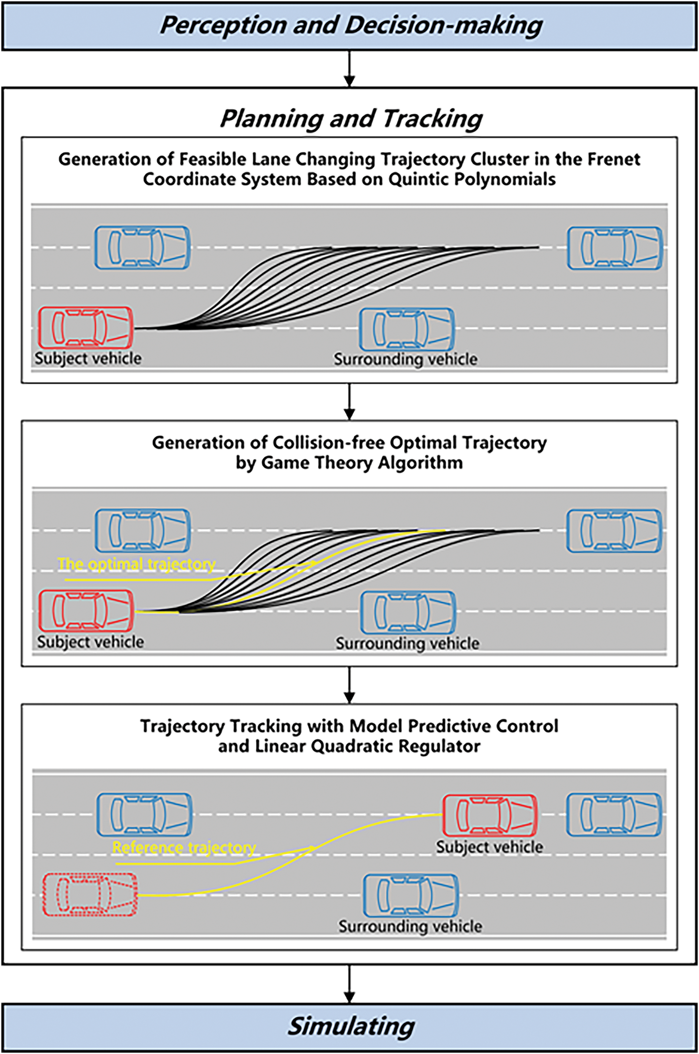
Figure 1: System framework for trajectory planning and tracking strategy

As shown in Fig. 1, the first step is to generate alternative trajectory clusters for different boundary conditions. Trajectory planning is carried out in the Frenet coordinate system using a fifth-degree polynomial and generates clusters of feasible trajectories that satisfy the horizontal and vertical boundary conditions.

The next step is to select collision-free trajectories from the alternative trajectory clusters using a collision avoidance algorithm based on game theory. A benefit matrix is constructed to measure the lane-changing benefits, including safety benefits, comfort benefits and speed benefits. The optimal lane-changing trajectories are selected to achieve vehicle collision avoidance at the trajectory planning level.

The final step is trajectory tracking by model predictive control (MPC) and linear quadratic regulator (LQR). In Fig. 1, the first step is performed by a decision mechanism based on a driving behaviour decision tree not discussed in this paper. It simplifies the vehicle operating state into three driving states: lane keeping, adaptive cruise and gaming lane-changing, analyses the lane-changing vehicles and the surrounding vehicles in each driving state, and performs threshold calculations. When a lane-changing is determined based on the threshold value, these three modules are executed sequentially with variable trigger times.

3  Generation of Alternative Trajectory

3.1 Constructing Trajectory Planning Sets

Traditional vehicle system modelling relies on geodetic coordinate systems, body coordinate systems and polar coordinates. As the motion trajectory of the self-driving vehicle grows, the trajectory becomes more difficult to fit and the cumulative error of the calculation increases. The Frenet coordinate system has excellent decoupling ability, which can plan the vehicle’s longitudinal and transverse motions independently and separately [24]. It can drastically improve the performance of decision models.

The polynomial-based lane change trajectory computation requires only the initial and target states of the vehicle. In the lane-changing scenario, there are FV (Front Vehicle) and RV (Rear Vehicle) in front and rear of the target lane, PV (Preceding Vehicle) in front of the current lane, and LV (Lane-changing Vehicle) in the current lane. Set Hfs as the safe lane-changing distance between LV and FV, Hfs = v·1.5·7/8; set Hrs as the safe lane-changing distance between LV and RV, Hrs = v·1.5·5/8. v is the vehicle speed, and the time interval between vehicles is 1.5 s. When the actual distances between LV, FV and RV are greater than the safe lane-changing distances, lane-changing planning is performed. The vehicle state at this time is the initial state. The target state is initially selected considering the predicted trajectory of the other vehicles in the target lane. The target state is finally adjusted by the safety constraints described below. As shown in Fig. 2, the boundary conditions in a complete lane-changing process can be expressed in terms of vertical and horizontal constraints as follows:

{S(0)=s0,S˙(0)=vs0,S¨(0)=as0,d(0)=d0,d˙(0)=vd0,d¨(0)=ad0S(τ)=sτ,S˙(τ)=vsτ,S¨(τ)=asτ,d(τ)=dτ,d˙(τ)=vdτ,d¨(τ)=adτ(1)

where S and d are the longitudinal and lateral distances of the vehicle along the reference path in the Frenet coordinate system, respectively. τ is the lane-changing duration.

Figure 2: Trajectory planning constraint

To facilitate solving for the curvature of the planned trajectory, the lateral boundary conditions are expressed by the geodetic to Frenet coordinate system transformation formula as [25]:

d(s0)=d0,d˙(s0)=vd0vs0,d¨(s0)=ad0−d˙(s0)⋅as0vs0,d(sτ)=dτ,d˙(sτ)=vdτvsτ,d¨(sτ)=adτ−d˙(sτ)⋅asτvsτ(2)

The fifth-degree polynomial plan obtained by re-coupling the vertical and horizontal boundary conditions is:

{S(t)=a0+a1⋅t+a2⋅t2+a3⋅t3+a4⋅t4+a5⋅t5d(s)=b0+b1⋅s+b2⋅s2+b3⋅s3+b4⋅s4+b5⋅s5(3)

where S(t) and d(t) are the coordinates of the vehicle mass center at time t in the Frenet coordinate system. a0, …, a5 and b0, …, b5 are the polynomial coefficients.

θh is the heading angle of the vehicle on the planning trajectory at any moment during the planning period. kh is the curvature of the vehicle on the planning trajectory at any moment during the planning period, which can be represented by Fig. 2 as:

tan⁡(θh)=limt→0d(n+t)−d(n)S(n+t)−S(n)=d(d(S))dS(4)

kh=d′′(S)(1+(d′(S))2)1.5(5)

As shown in Fig. 3, different alternative target points can be taken before and after the target point (Sτ, dτ) to get the alternative trajectory set in trajectory planning.

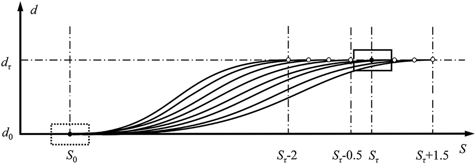
Figure 3: Alternative set of trajectories in Frenet coordinate system

3.2 Vehicle Dynamics Modelling in the Frenet Coordinate System

In order to clearly describe the motion law of the vehicle, as shown in Fig. 4, a two-degree-of-freedom vehicle dynamics model is established as follows [26]:

[y¨φ¨]=[Cαf+CαrmvxaCαf−bCαrmvx−vxaCαf−bCαrIvxa2Cαf+b2CαrIvx][y˙φ˙]+[−CαfmCαfI]δ(6)

where vx is the component of v in the x-direction, Cαf and Cαr are the lateral stiffnesses of the front and rear wheels, a and b are the distances of the vehicle’s center of gravity from the front and rear axles, I is the rotational moment of inertia of the whole vehicle, and m is the vehicle mass. The vehicle parameters are in Table 1. As shown in Fig. 4, αf and αr are the front and rear wheel lateral deflection angles, Fyf and Fyr are the front and rear axle lateral forces, δ is the turning angle of the driving wheels, φ is the transverse pendulum angle, and β is the lateral deflection angle of the center of mass. It is usually assumed that cos(δ) = 1.

Figure 4: Two-Degrees-of-Freedom (2-DOF) vehicle dynamic model

Once again, through the coordinate transformation, the vehicle system dynamics in the Frenet coordinate system can be obtained as follows:

e˙r=A⋅er+B⋅δ+C⋅θ˙r(7)

where

er=[ede˙deφe˙φ]′,u=δ,ed=d,eφ=φ−θr,

A=[01000Cαf+Cαrmvx−Cαf+CαrmaCαf−bCαrmvx00010aCαf−bCαrIvx−aCαf−bCαrIa2Cαf+b2CαrIvx],B=[0−Cαfm0−a⋅CαfI],C=[0aCαf−bCαrmvx−vx0a2Cαf+b2CαrIvx].

er is the new state variable, u is the control vector, ed is the lateral error, eφ the heading error, and θr is the angle between the reference heading angle at the vehicle projection point and the x-axis of the Cartesian coordinate system.

4  Selection of Optimal Trajectories

4.1 Revenue Matrix Design

Game theory can be classified into non-cooperative and cooperative games based on the ability to form binding agreements between participants. Because vehicles travelling on non-smart networked roads cannot share the driving strategies of other vehicles, the lane-changing game discussed in this paper is a non-cooperative game. During the game, each participant prioritizes their payoffs. In such Prisoner’s Dilemma situations, the Nash equilibrium is a suboptimal solution acceptable to all participants [27]. During lane-changing, vehicles are concerned with metrics such as safety, comfort, and speed payoffs [28]. The payoffs from adopting different strategies vary, so a payoff function needs to be designed to include the set of strategies among all participants [29].

The LV’s lane change strategy is divided into two types, lane change and keep moving, which are set to C and N, respectively. The corresponding probabilities are l1 and l2 (l1 + l2 = 1), respectively. FV and RV have both incentive and disincentive strategies for lane-changing. Their corresponding probabilities are f1, f2 (f1 + f2 = 1), r1, and r2 (r1 + r2 = 1), respectively. When LV makes different strategies, the payoff matrix is shown in Table 2.

When there is only FV or RV in the target lane, it is a two-party game. When both cars exist, to improve driving safety and traffic efficiency, this model assumes that the two vehicles maintain goal consistency. It can still be regarded as a two-party game, which simplifies the complexity of the game and also considers the impact of FV and RV on lane changing. Table 2 shows the two-party game payoff matrix. The following equation gives the payoffs for the three vehicles with different strategies:

[LijFijRij]=α[EsLijEsFijEsRij]+β[EvLijEvFijEvRij]+γ[EaLijEaFijEaRij](8)

where Lij, Fij, and Rij denote their payoffs. EsLij, EvLij, and EaLij denote LV’s safety, speed and comfort payoff, respectively. FV and RV are similar to LV, α, β, and γ are regulation factors.

4.2 Payoff Function Design

The positions of the vehicles participating in the game before and after the lane-changing are shown in Fig. 5. Taking LV as an example, L0 and Lτ denote the position of LV before and after the change of channel.

Figure 5: Position of participating vehicles in the game before and after lane-changing

Es is the safety payoff and is understood as the safety space expansion factor for the corresponding vehicle before and after lane-changing. Similarly, Ev is the speed payoff and is embodied as the spatial potential for acceleration of the corresponding vehicle before and after the adoption of the corresponding strategy. Es and Ev are defined as:

{EsL=min(|Lτ−Rτ|,|Lτ−Fτ|,|Lτ−Pτ|)min(|L0−R0|,|L0−F0|,|L0−P0|)EsF=min(|Fτ−Rτ|,|Fτ−Lτ|)min(|F0−R0|,|F0−L0|)EsR=min(|Rτ−Fτ|,|Rτ−Lτ|)min(|R0−F0|,|R0−L0|)(9)

{EvL=|Fτ−Lτ||P0−L0|EvF=EvL+EvR2EvR=|Lτ−Rτ||F0−R0|(10)

where vL and vR are the LV and RV vehicle speeds, respectively. Because the speed payoff for FV is not probable, the average speed payoff for LV and RV is assigned to EvF. Ea is the comfort payoff, which expresses the change in acceleration of the vehicle when the strategy is taken and is defined as follows:

{EaL=1∫0Td⃛(t)2dt+∫0TS⃛(t)2dtEaF=0EaR=0(11)

The overall payoffs before and after changing lanes are focused on LV, the size of which is determined by EsL and EvL. When EsL = 1 and EvL = 1, there are no payoffs to safety space and acceleration space potential, regardless of whether the vehicle changes lanes. Thus, the lane-changing strategy probability is obtained by ab normalization.

{l1={0,(EsL⋅EvL≤lD)EsL⋅EvL−lDlU−lD,(lD<EsL⋅EvL<lU)1,(lU≤EsL⋅EvL)l2=1−l1(12)

where lU > 1, 0 < lD < 1. lU and lD are the maximum and minimum values set during the normalization process. LV’s lane-changing aggressiveness is determined by its values; the smaller all values are, the more this vehicle tends to change lanes in the game.

The respective strategy probability for FV and RV is calculated similarly for LV. The relative position change between vehicles measures the strategies adopted by competing vehicles. At the initial stage of lane change the changes in the position, velocity, and acceleration of the LV are small and complex. The PV will not actively respond to the behavior of the LV, and the stability of the PV can be obtained through the onboard sensors. Using PV instead of LV as the calculation anchor can also express relative distance changes. And enlarge the calculation target and improve the calculation efficiency.

As shown in Fig. 6, the position of each vehicle change in a short period after the LV gives the intention to change lane is used to calculate the strategy probabilities of FV.

{f1={0,(Ff≤fD)Ff−fDfU−fD,(fD<Ff<fU)1,(fU≤Ff)f2=1−f1Ff=EsF⋅EvF⋅|Pt−Rt||P0−R0|(13)

where fU and fD are the extremes set during the normalization process. Strategy probability for RV is calculated in the same way. Their value determines the tolerance of competing vehicles for lane-changing aggressiveness; the closer the upper and lower limits are, the more sensitive the aggressiveness judgements of competing vehicles becomes.

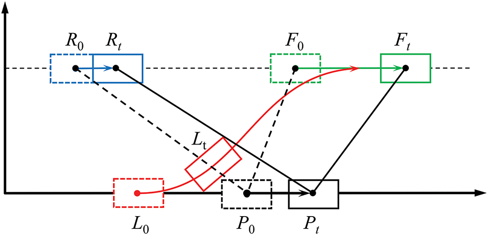
Figure 6: Prediction of aggressiveness

4.3 Nash Equilibrium

The mixed expected payoffs under each strategy combination are:

{EL(l,f,r)=∑i=12li[(∑j=i2fj⋅Lij)+(∑j=i2rj⋅Lij)]EF(l,f,r)=∑i=12li(∑j=i2fj⋅Lij)ER(l,f,r)=∑i=12li(∑j=i2rj⋅Rij)(14)

where EL, EF, and ER denote their mixed expected payoffs. When the set of strategies is finite, there must exist an optimal solution for the game model, where all participants can achieve maximum returns when adopting these strategies. The maximum value of each participant’s expected payoff can be computed by Eq. (15). By letting the mixed probability of maximum payoff be (l*, f*, r*), the following equation can be obtained:

{EL(l∗,f∗,r∗)≥EL(l,f∗,r∗)EF(l∗,f∗,r∗)≥EF(l∗,f,r∗)ER(l∗,f∗,r∗)≥ER(l∗,f∗,r)(15)

The resulting l*, f*, and r* are the Nash equilibrium solutions for the three vehicles in the game’s current state. Focusing only on LV’s payoff during lane-changing, the maximum payoff table for all optimal strategies in the strategy set of LV can be obtained. The maximum payoff determines the lane-changing strategy and optimal trajectory.

4.4 Validity Verification

There are three types of game participants in this article: (1) only FV (2) only RV, (3) both FV and RV. Trajectory planning from initial to target state, with the subject vehicle speed of 60 km/h and the curvature of 1/300 m−1 on the bend. Difine the individual payoff weights and aggressiveness prediction parameters, lU = 1.2, lD = 0.8, fU = 1.3, fD = 0.8, rU = 1.3, rD = 0.7.

(1)   The first scenario is ‘on FV’. In this scenario, there is FV ahead of the target lane, indicating that the presence of acceleration space is crucial for lane-changing behaviour. The payoff of safety, speed, and comfort are respectively: α = 0.3, β = 0.5, γ = 0.2. The payoff matrix for this vehicle can be obtained by performing a blended expected payoff calculation from the payoff matrices of all strategies, as shown in Tables 3 and 4. The optimal trajectory is the alternative trajectory #4, with the largest payoff during the lane-changing game. LV has the best safety, comfort, and acceleration potential in this condition. Fig. 7 shows the performance of the optimal trajectory in different coordinate systems. In curved road scenarios, the Frenet coordinate system can simplify complex path problems. In the initial stage, the Cartesian coordinate system is converted to the Frenet coordinate system, and the conversion error is taken into account. It is particularly suitable for the set highway scene and can achieve higher trajectory tracking accuracy. The Cartesian coordinate system more clearly shows the actual planned trajectory and driving trajectory. It is more intuitive and easier to determine whether a collision occurs.

(2)   The second scenario is ‘on RV’. This scene only has rear vehicles in the target lane, and the priority of acceleration space is lower than in the previous scene. The payoffs of safety, speed, and comfort are respectively: α = 0.3, β = 0.3, γ = 0.4. At this point, it is a two-car game, hence Fij = 0, as shown in Table 5. The game result is that the optimal trajectory is the alternative trajectory #5. It was verified that the model can change weights to generate different driving strategies. In practice, the weights in the payoff matrix can be dynamically adjusted through machine learning methods to adapt to different driving scenarios. Compared to the previous scenario, the alternative trajectory sets are denser in Fig. 8a, which is consistent with the calculation results presented in Table 4.

(3)   The third scenario is ‘both FV and RV’. When there are cars in front and behind the target lane, the space at the beginning of the game is relatively small. The presence of the vehicle in front of the target lane makes the importance of acceleration space the same as in scenario 1. The presence of a vehicle behind makes the potential danger of lane change higher than that of a single-vehicle scenario. Therefore, the payoffs of safety, speed, and comfort are respectively: α = 0.35, β = 0.5, γ = 0.15, as shown in Table 6. Fig. 9 and Table 4 show that the strategy can effectively calculate the optimal trajectory.

Figure 7: (a) Cartesian coordinate system planning trajectories; (b) Frenet coordinate system planning trajectories

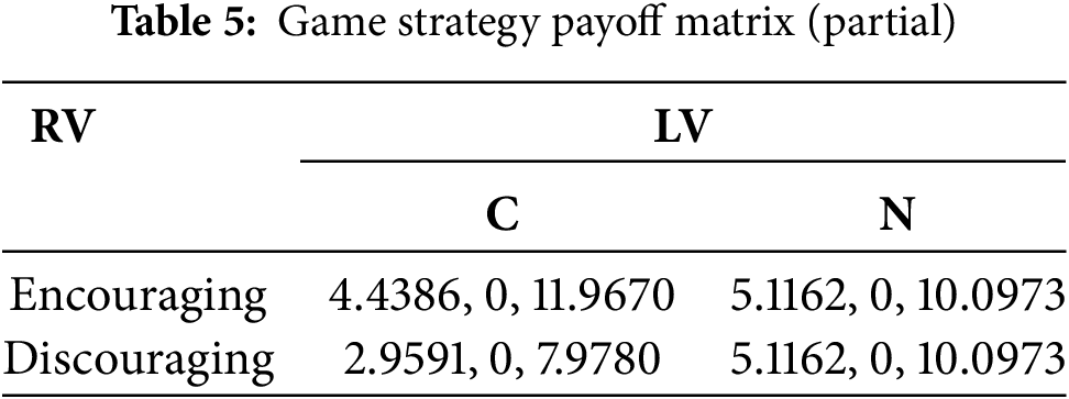
Figure 8: (a) Cartesian coordinate system planning trajectories; (b) Frenet coordinate system planning trajectories

Figure 9: (a) Cartesian coordinate system planning trajectories; (b) Frenet coordinate system planning trajectories

To evaluate whether the optimal trajectory is applicable to real traffic, the NGSIM data is used for validation. NGSIM is a general tool that collects video to capture real traffic information and verify the effectiveness of trajectory planning. The data used mainly includes road data and status data of related vehicles. A series of vehicles with lane-changing behaviors are selected as target vehicles in NGSIM. The evaluation is performed by calculating the overlap rate and similarity between the actual trajectory and the planned trajectory.

Fig. 10 shows a representative trajectory planning diagram. The red curve is an actual left lane change trajectory in the NGSIM dataset. Select the target vehicle, surrounding vehicles, and road status information when the lane change starts. The blue curve represents the trajectory planned by substituting this information into the model. Find overlapping points by computing the closest point match between two trajectory point sets. The distance threshold is set to 0.3 m. Points less than this threshold are considered to be overlapping points. The overlap rate of the two trajectories shown in Fig. 10 is 88.7%. The Euclidean distance between two trajectory points is calculated, and the root mean square error (RMSE) is used to quantify the difference between the trajectories. The smaller the RMSE, the more similar the trajectories are. The RMSE of the planned trajectory shown in Fig. 10 is 0.1371. Trajectories with overlap greater than 80% and RMSE less than 0.2 were considered usable plans. Table 7 shows that there are 110 trajectories available for this model, and the lane-changing accuracy is 82.7%.

Figure 10: Trajectory comparison

5  Trajectory Tracking Control Algorithm

5.1 LQR Tracking Algorithm

Since the actual system is discrete, Eq. (7) needs to be converted to a discrete-time model. Defining the sampling time as Tsa and the time step as k, the discrete-time model is expressed as:

e(k+1)=A¯⋅e(k)+B¯⋅u(k)(16)

where A¯=A⋅Tsa+I,B¯=B⋅Tsa, I is the unit matrix. Define the cost function:

JL=∑k=0+∞(e(k)T⋅Q⋅e(k)+u(k)T⋅R⋅u(k))(17)

where Q and R are the state weighting matrix and control weighting matrix, which influence the rate at which deviations converge to zero and the magnitude of the control inputs.

For closed-loop control, construct the Hamiltonian function. Multiplying the front of the constraint equation by the covariance matrix λ yields the Hamilton function as follows:

H(k)=e(k)T⋅Q⋅e(k)+u(k)T⋅R⋅u(k)+λ(k+1)T⋅(A¯⋅e(k)+B¯⋅u(k))(18)

Performance metrics rewritten according to system constraints and design control laws.

JL=∑k=0n−1(H(k)−λ(k+1)T⋅e(k+1))+e(k)T⋅Q⋅e(k)(19)

u(k)=−R−1⋅B¯Tsa⋅λ(k+1)(20)

Construct the Riccati differential equation, where P(k) is a semi-positive definite symmetric matrix, λ(k)=P(k)⋅e(k).

PA+ATP−PBR−1BPT+Q=0(21)

The control law and final state feedback control are calculated as follows:

u(k)=−R−1⋅BT⋅P(k)⋅e(k)(22)

UL=−K⋅er(23)

where K is a 1 × 4 matrix, denoting the gain of the LQR controller.

Solving the Riccati differential equation offline improves the speed of solving the system controller. Create a look-up table of feedback gain coefficients for different vehicle speeds. This offline look-up table approach improves the system computation speed and enhances the real-time performance of the control system.

5.2 MPC Tracking Algorithm

On this basis of Eq. (17), the equations for predicting the future system output can be derived. In order to unify e(k) and u(k − 1), let ξ(k) be the new state variable and η(k) be the system output η(k), which leads to the state space expression:

{ξ(k+1)=A~⋅ξ(k)+B~⋅Δu(k)η(k)=C~⋅ξ(k)(24)

where ξ(k)=[e(k)u(k−1)],Δu(k)=u(k)−u(k−1),A~=[A¯B¯0I],B~=[B¯I],C~=[I0]

Hp is the system prediction time domain, and Hc is the control time domain, where k = Hc, Hc + 1, …, Hp − 1. The prediction model is obtained by iteration.

Y(k+1|k)=Φ⋅ξ(k)+Θ⋅ΔU(k)(25)

Similar to Eq. (20), the cost function in the prediction process is defined as:

JM=Y(k)T⋅QQ⋅Y(k)+ΔU(k)T⋅RR⋅ΔU(k)(26)

QQ and RR are the state weighting matrix and control weighting matrix. The following are essential regarding vehicle driving effects: steering angle constraints, steering angle increment constraints, and acceleration constraints. Considering the need to improve the smoothness of the vehicle travelling and to fit the desired path, the amount of control and the control increments are also constrained.

{umin(k+i)≤u(k+i)≤umax(k+i),i=0,…,Hc−1Δumin(k+i)≤Δu(k+i)≤umax(k+i),i=0,…,Hc−1(27)

On this basis, the quadratic objective function can be obtained as follows [30]:

JM=ΔU(k)T⋅Ht⋅ΔU(k)+Gt⋅ΔU(k)(28)

where Ht=ΘT⋅QQ⋅Θ+RR, Gt=2(Φ⋅ξk)T⋅QQ⋅Θ.

The optimal sequence of ΔU(k) is obtained by solving for the minimum value of JM under constraints Eq. (27). The control input for time step k is obtained by iteration:

u(k|k)=u(k−1|k)+[10⋯0]δU∗(k)(29)

where ΔU*(k) denotes the optimal sequence of ΔU(k).

6  Simulations and Discussion

This section first verifies the effectiveness of the LQR and MPC trajectory tracking controllers. The simulation platform of MATLAB and CarSim is built for simulation verification, and the vehicle parameters are shown in Table 1. The single shift line in the straight road environment and the single shift line trajectory in the curved road environment were used as reference trajectories. Further experimental tests were conducted on a driving simulator. The feasibility and effectiveness of the proposed lane-changing strategy under complex working conditions are verified. The feasibility and real-time implementation capability of the proposed algorithm are demonstrated.

6.1 Verification of Single Shift Line on Straight Road

Experimental validation was carried out under straight road single shift line conditions, as shown in Fig. 11. In straight-line scenarios, the Cartesian coordinate system is used directly for planning and control. The coordinate conversion step can be omitted, which reduces errors and optimizes calculation speed. Where the speed of the subject vehicle is 100 km/h, the road friction coefficient is 0.75, the lane width is 3.6 m, and the sampling time is 0.01 s. Fig. 11a shows the lateral displacement of the subject vehicle relative to the road edge line Y. Fig. 11b–d illustrates the yaw angle, front wheel angle of rotation, and lateral acceleration of the subject vehicle, respectively.

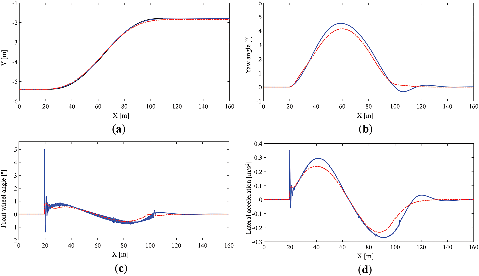
Figure 11: (a) Lateral displacement; (b) Yaw angle; (c) Front wheel angle; (d) Lateral acceleration

In detail, the black line represents the planning trajectory, the blue line represents the simulation of LQR tracking, and the red line represents the simulation of MPC tracking. The lateral displacement shows that the LQR and MPC controllers do well in tracking the planned trajectory. Compared to the LQR control, the vehicle lateral error under MPC control is greater, up to a maximum of 0.2 m. The vehicle sway angle shows that the vehicle controlled by the MPC controller has a smaller peak sway angle and better stability during lane-changing. The front wheel angle of the vehicle shows that the vehicle starts to change lanes at 20 m and completes the change at around 85 m. In this case, the front wheel angle of the vehicle controlled by the MPC controller is smoother, with a sudden change in the initial phase of lane-changing and a maximum value of no more than 1° during the process. In contrast, the control of the front wheel angle by the LQR controller suffers from the jitter phenomenon. The lateral acceleration curve shows that both the LQR and MPC controllers have lateral acceleration within 0.3 g during vehicle lane-changing. Moreover, the lateral acceleration profile of the vehicle controlled by the MPC controller is smoother, indicating good comfort.

6.2 Verification of Single Shift Line on Curved Road

Similar to the straight road, the vehicle state response curve under single shift condition of constant curvature curved road can be obtained in Fig. 12. The radius of curvature of the road is 300 m.

Figure 12: (a) Lateral displacement; (b) Yaw angle; (c) Front wheel angle; (d) Lateral acceleration

Like state response curve for a curved road would result in proportional compression if the identical X is taken as the transverse axis, so the longitudinal displacement S in the Frenet coordinate system is taken as the transverse axis in describing the vehicle’s transverse swing angle, front wheel angle of rotation, and transverse acceleration.

The tracking effect of curved roads is similar to that of straight roads. Fig. 12b–d shows that the vehicle starts to change lanes at 40 m and completes the change at around 140 m, in which the front wheel angle of the vehicle controlled by the MPC controller is stable in the interval of 1°–2° change during the initial phase of the lane-changing. The LQR controller’s front wheel angle judder is still present and severe. The lateral acceleration change is slightly larger than the straight line but still within control. Furthermore, MPC control is still better than LQR control. Therefore, a dual controller trajectory tracking approach is used, with the MPC controller for the lane-changing process and the LQR controller for the road-holding process. It can effectively increase the speed of calculation.

6.3 Lane-Changing Strategy Verification under Complex Road Conditions

In this subsection, the effectiveness of the lane-changing strategy is further validated through hardware-in-the-loop driving simulator experiments. The hardware-in-the-loop driving simulator shown in Fig. 13 consists of a model Lenovo ThinkCentre M910t-D158 host computer, a model HP Compaq DC7700p CMT implementation target machine, five joint flat-screen displays, sensors, motors, and acquisition cards. The real-time system is built with LabVIEW Real-Time module as the software core.

Figure 13: Autopilot simulator

In the experiment, the driving route was set up as an S-shaped road with straight and left and right curves. In order to validate the effectiveness of the driving scheme, game lane-changing, adaptive cruise, lane-changing abort, and direct lane-changing are implemented continuously for four working conditions.

Fig. 14 shows that the black line is the expected steering wheel angle, and the red line is the actual steering wheel angle. The steering wheel angle during lane-changing can achieve a better tracking effect. In conjunction with the in-software timer, at 6.392 s, the following threshold is calculated to be zero, the lane-changing speed threshold to be one, and the lane-changing distance threshold to be zero. The game lane change is performed, as shown in Fig. 14a, and the lane change is performed at 6.392~9.557 s.

Figure 14: (a) Steering wheel angle in game changing lane; (b) Steering wheel angle in adaptive cruise control; (c) Steering wheel angle in lane-changing stop; (d) Steering wheel angle in direct lane change

At 9.557 to 23.712 s, the calculation of the following and lane-changing speed threshold is zero. In the process, the subject vehicle enters the curve and gets closer to the vehicle in front of it, but there is no opportunity to change lanes. Adaptive cruise is maintained to follow the vehicle in front based on driving behaviour decisions. The actual and desired steering wheel angle is within 1°, as shown in Fig. 14b.

At 23.712 s, by calculating the thresholds, this vehicle again generates the intention to change lanes and starts a two-sided game with the vehicle behind the target lane. 24.6–25.8 s, the speed of the vehicle behind the target lane increases from 90 to 110 km/h. At 25.843 s, based on the calculation of the abort threshold of 1, the lane-changing abort command is triggered, and the vehicle immediately returns to the original lane. The steering wheel angle deviation is not more than 1.5°, as shown in Fig. 14c. The actual tracking effect is satisfactory for sudden changes in steering wheel angle within 0.5 s.

At 29.829 s, by calculating the lane-changing distance threshold, which is zero, indicating that there are no gaming vehicles, this vehicle adopts a direct lane-changing strategy. As shown in Fig. 14d, the two curves coincide, and the steering wheel angle changes smoothly during the lane-changing.

The simulations were run on a desktop computer with an Intel Core i7-12700KF (3.6 GHz), 32.0 GB RAM, Microsoft Windows 10 (64-bit), and MATLAB 2016b (64-bit). The key indicators are shown in Table 8. Lane-changing conditions are divided into the straight road and the curved road. The maximum safety distance meets the safe driving conditions. The maximum acceleration on curved roads is less than 0.52°, ensuring driving stability. The average error is within the controllable range of 0.5 m. The total computation time for the two cases including planning and control is 0.642 and 0.813 s, respectively.

The LQP controller has a small amount of calculation while the MPC controller has a higher calculation complexity. In most cases, the LQR controller provides good performance in real-time systems. The MPC controllers require stronger computing resources. Adaptive optimization algorithms and machine learning-assisted optimization controller design and parameter selection are future research directions.

7  Conclusion

This paper proposes a lane change decision system for trajectory planning and tracking control of intelligent vehicles. The quintic polynomial is used for vehicle trajectory planning on straights and curves. On this basis, the trajectories are evaluated according to a game-theoretic approach. An automated driving simulation platform is built based on hardware-in-the-loop technology, and automated driving in simple traffic is achieved. The experimental results show that the strategy can plan an optimal lane change trajectory with collision avoidance capability while balancing safety, acceleration, and comfort. Future works will focus on optimizing the algorithms and the driving simulator’s data communication architecture to improve real-time performance further.

Acknowledgement: This paper grateful thanks to all reviewers for their selfless contributions to science and to all editors for their outstanding work in improving the quality of the paper.

Funding Statement: This work is supported by the Science and Technology Program of Shandong Higher Education Institutions (Grant J18KA048).

Author Contributions: The authors confirm contribution to the paper as follows: study conception and design: Buwei Dang, Huanming Chen, Heng Zhang; data collection: Jixian Wang, Jian Zhou; analysis and interpretation of results: Buwei Dang, Jian Zhou; draft manuscript preparation: Buwei Dang, Huanming Chen. All authors reviewed the results and approved the final version of the manuscript.

Availability of Data and Materials: The authors confirm that the data supporting the findings of this study are available within the paper.

Ethics Approval: Not applicable.

Conflicts of Interest: The authors declare no conflicts of interest to report regarding the present study.

References

1. Zhou J, Zheng H, Wang J, Wang Y, Zhang B, Shao Q. Multiobjective optimization of lane-changing strategy for intelligent vehicles in complex driving environments. IEEE Trans Veh Technol. 2020;69(2):1291–308. doi:10.1109/TVT.2019.2956504. [Google Scholar] [CrossRef]

2. Ersal T, Kolmanovsky I, Masoud N, Ozay N, Scruggs J, Vasudevan R, et al. Connected and automated road vehicles: state of the art and future challenges. Veh Syst Dyn. 2020;58(5):672–704. doi:10.1080/00423114.2020.1741652. [Google Scholar] [CrossRef]

3. Montanaro U, Dixit S, Fallah S, Dianati M, Stevens A, Oxtoby D, et al. Towards connected autonomous driving: review of use-cases. Veh Syst Dyn. 2019;57(6):779–814. doi:10.1080/00423114.2018.1492142. [Google Scholar] [CrossRef]

4. Nadeem Ahangar M, Ahmed QZ, Khan FA, Hafeez M. A survey of autonomous vehicles: enabling communication technologies and challenges. Sensors. 2021;21(3):706. doi:10.3390/s21030706. [Google Scholar] [PubMed] [CrossRef]

5. Arrigoni S, Braghin F, Cheli F. MPC trajectory planner for autonomous driving solved by genetic algorithm technique. Veh Syst Dyn. 2022;60(12):4118–43. doi:10.1080/00423114.2021.1999991. [Google Scholar] [CrossRef]

6. Badue C, Guidolini R, Carneiro RV, Azevedo P, Cardoso VB, Forechi A, et al. Self-driving cars: a survey. Expert Syst Appl. 2021;165:113816. doi:10.1016/j.eswa.2020.113816. [Google Scholar] [CrossRef]

7. Cao H, Zhao S, Song X, Bao S, Li M, Huang Z, et al. An optimal hierarchical framework of the trajectory following by convex optimisation for highly automated driving vehicles. Veh Syst Dyn. 2019;57(9):1287–317. doi:10.1080/00423114.2018.1497185. [Google Scholar] [CrossRef]

8. He Y, Feng J, Wei K, Cao J, Chen S, Wan Y. Modeling and simulation of lane-changing and collision avoiding autonomous vehicles on superhighways. Phys A Stat Mech Appl. 2023;609:128328. doi:10.1016/j.physa.2022.128328. [Google Scholar] [CrossRef]

9. Dixit S, Fallah S, Montanaro U, Dianati M, Stevens A, McCullough F, et al. Trajectory planning and tracking for autonomous overtaking: state-of-the-art and future prospects. Annu Rev Contr. 2018;45:76–86. doi:10.1016/j.arcontrol.2018.02.001. [Google Scholar] [CrossRef]

10. Wang Y, Wei C, Li S. QPNet: lane-changing trajectory planning combining quadratic programming and neural network under the convex optimization framework. IET Intell Transp Syst. 2022;16(11):1578–99. doi:10.1049/itr2.12234. [Google Scholar] [CrossRef]

11. Guo L, Ge PS, Yue M, Zhao YB. Lane changing trajectory planning and tracking controller design for intelligent vehicle running on curved road. Math Probl Eng. 2014;2014(1):478573. doi:10.1155/2014/478573. [Google Scholar] [CrossRef]

12. Suh J, Chae H, Yi K. Stochastic model-predictive control for lane change decision of automated driving vehicles. IEEE Trans Veh Technol. 2018;67(6):4771–82. doi:10.1109/TVT.2018.2804891. [Google Scholar] [CrossRef]

13. Zeng D, Yu Z, Xiong L, Zhao J, Zhang P, Li Z, et al. A novel robust lane change trajectory planning method for autonomous vehicle. In: 2019 30th IEEE Intelligent Vehicles Symposium; 2019 Jun 9–12; Paris, France. p. 486–93. doi:10.1109/ivs.2019.8814151. [Google Scholar] [CrossRef]

14. You F, Zhang R, Lie G, Wang H, Wen H, Xu J. Trajectory planning and tracking control for autonomous lane change maneuver based on the cooperative vehicle infrastructure system. Expert Syst Appl. 2015;42(14):5932–46. doi:10.1016/j.eswa.2015.03.022. [Google Scholar] [CrossRef]

15. Luo Y, Xiang Y, Cao K, Li K. A dynamic automated lane change maneuver based on vehicle-to-vehicle communication. Transp Res Part C Emerg Technol. 2016;62:87–102. doi:10.1016/j.trc.2015.11.011. [Google Scholar] [CrossRef]

16. Yang D, Zheng S, Wen C, Jin PJ, Ran B. A dynamic lane-changing trajectory planning model for automated vehicles. Transp Res Part C Emerg Technol. 2018;95:228–47. doi:10.1016/j.trc.2018.06.007. [Google Scholar] [CrossRef]

17. Wei C, Li S. Planning a continuous vehicle trajectory for an automated lane change maneuver by nonlinear programming considering car-following rule and curved roads. J Adv Transp. 2020;2020:8867447. doi:10.1155/2020/8867447. [Google Scholar] [CrossRef]

18. Kita H. A merging-giveway interaction model of cars in a merging section: a game theoretic analysis. Transp Res Part A Policy Pract. 1999;33(3–4):305–12. doi:10.1016/S0965-8564(98)00039-1. [Google Scholar] [CrossRef]

19. Ding N, Meng X, Xia W, Wu D, Xu L, Chen B. Multivehicle coordinated lane change strategy in the round about under Internet of vehicles based on game theory and cognitive computing. IEEE Trans Ind Inform. 2020;16(8):5435–43. doi:10.1109/TII.2019.2959795. [Google Scholar] [CrossRef]

20. Yu H, Tseng HE, Langari R. A human-like game theory-based controller for automatic lane changing. Transp Res Part C Emerg Technol. 2018;88:140–58. doi:10.1016/j.trc.2018.01.016. [Google Scholar] [CrossRef]

21. Guo W, Cao H, Song X, Wang J, Zhao S, Yi B. Adaptive authority allocation for shared steering control considering social behaviours: a hybrid fuzzy approach with game-theoretical vehicle interaction model. Veh Syst Dyn. 2024;62(5):1203–29. doi:10.1080/00423114.2023.2220840. [Google Scholar] [CrossRef]

22. Lopez VG, Lewis FL, Liu M, Wan Y, Nageshrao S, Filev D. Game-theoretic lane-changing decision making and payoff learning for autonomous vehicles. IEEE Trans Veh Technol. 2022;71(4):3609–20. doi:10.1109/TVT.2022.3148972. [Google Scholar] [CrossRef]

23. Cheng G, Sun Q, Bie Y. Mandatory lane-changing modelling based on a game theoretic approach in traditional and connected environments. Transp Saf Environ. 2023;5(1):tdac035. doi:10.1093/tse/tdac035. [Google Scholar] [PubMed] [CrossRef]

24. Werling M, Ziegler J, Kammel S, Thrun S. Optimal trajectory generation for dynamic street scenarios in a Frenét frame. In: 2010 IEEE International Conference on Robotics and Automation ICRA; 2010 May 3–7; Anchorage, AK, USA. p. 987–93. doi:10.1109/ROBOT.2010.5509799. [Google Scholar] [CrossRef]

25. Xing X, Zhao B, Han C, Ren D, Xia H. Vehicle motion planning with joint Cartesian-frenét MPC. IEEE Robot Autom Lett. 2022;7(4):10738–45. doi:10.1109/LRA.2022.3194330. [Google Scholar] [CrossRef]

26. Zheng H, Zhou J, Li B. Design of adjustable road feeling performance for steering-by-wire system. SAE Int J Veh Dyn Stab NVH. 2018;2(2):121–34. doi:10.4271/10-02-02-0008. [Google Scholar] [PubMed] [CrossRef]

27. Qu D, Zhang K, Song H, Jia Y, Dai S. Analysis and modeling of lane-changing game strategy for autonomous driving vehicles. IEEE Access. 2022;10:69531–42. doi:10.1109/ACCESS.2022.3187431. [Google Scholar] [CrossRef]

28. Hang P, Lv C, Xing Y, Huang C, Hu Z. Human-like decision making for autonomous driving: a noncooperative game theoretic approach. IEEE Trans Intell Transp Syst. 2021;22(4):2076–87. doi:10.1109/TITS.2020.3036984. [Google Scholar] [CrossRef]

29. Ali Y, Zheng Z, Haque MM, Wang M. A game theory-based approach for modelling mandatory lane-changing behaviour in a connected environment. Transp Res Part C Emerg Technol. 2019;106:220–42. doi:10.1016/j.trc.2019.07.011. [Google Scholar] [CrossRef]

30. Zhu M, Chen H, Xiong G. A model predictive speed tracking control approach for autonomous ground vehicles. Mech Syst Signal Process. 2017;87:138–52. doi:10.1016/j.ymssp.2016.03.003. [Google Scholar] [CrossRef]