An Enhanced Fuzzy Routing Protocol for Energy Optimization in the Underwater Wireless Sensor Networks

1  Introduction

Underwater control and monitoring systems are among the challenging topics in electronics and computer sciences. It has been discussed that the lower the cost-to-efficiency ratio under the same working conditions and quality, the greater the popularity of that method. The equipment known as a sensor can be used to monitor changes in the surrounding environment or the status of each set [1,2]. Every sensor can sense and present changes in the desired environment using specific parameters such as temperature, humidity, and pressure. For example, monitoring and controlling the underwater environment is feasible using information from sensors embedded in the water. The data link layer protocol is responsible for coordinating the access of nodes to the shared wireless media in underwater sensor networks with high throughput and energy efficiency. Network nodes can share a broadcast channel through a media access control protocol [3,4]. For its core functionality, the Medium Access Control (MAC) protocol is developed to prevent concurrent data transmissions and manage packet collision resolution [5]. Additionally, it ensures energy efficiency, minimizes channel access delays, and maintains a balanced load across network nodes. Due to the harsh and weak underwater audio channels, the Media Access Control layer protocol is critical in using the underwater sensor network. Developing an interlayer protocol is a significant challenge in developing underwater sensors. It is ideal for an interlayer protocol (between the network and the data link layer) to simultaneously provide optimal underwater media access control with high throughput, low energy consumption, and high-reliability paths for data exchange to select the desired destination [6]. Due to the strain on the medium in underwater sensor networks (UWSNs), the transmission speed of audio frequency is significantly reduced. The delays in the transmission and distribution of information packets in this network will result in the packets not reaching their intended recipients on time, and the meetings between the networks will be lost due to the delays in transmission and distribution. Instead, the simultaneous sending of neighbors, known as hidden terminal, results in congestion in the media environment and noise passing through the surface. As determined by the above decision, crowding and collision are the most significant challenges facing underwater sensor networks. Path congestion, collisions, and queue slippage will also be added to these challenges in the following stage. To address the issues and problems raised in this research, a method is proposed to prevent congestion and, in the event of congestion, a way to reduce and address it. Additionally, we would like to avoid time waste by dynamically varying the work cycle time of meetings between the neighbors of the member nodes of the main paths [7].

Motivation and Contributions

Developing UWSNs faces significant challenges due to a few factors, e.g., adverse node positioning, environmental noise interference, and Doppler frequency shifts, all of which negatively impact network throughput, data transmission efficiency, and communication reliability. These factors make data transmission to the central node collecting data (Sink) particularly challenging. Consequently, effective route planning is essential to ensure seamless data propagation from nodes to the sink. However, deep-water environments inherently exhibit slow data propagation speeds which leads to high energy consumption for inter-node communication. Furthermore, UWSNs operate within a dynamic and complex system, distinct from Terrestrial Wireless Sensor Networks (TWSNs) due to their lower energy consumption and reduced latency. Given the harsh underwater conditions, it is fundamental to develop highly secure and efficient network links [8]. To ensure network reliability during emergencies, underwater routing protocols must be adaptable to frequent topology modifications. The routing protocol plays a critical role in determining how data is transmitted between underwater source nodes and surface destination nodes. With increasing research interest in UWSNs, a growing number of studies focus on specific aspects of routing protocols, such as energy consumption or geographic location. However, most existing surveys lack a comprehensive comparative analysis of multi-path underwater routing protocols, which leaves a gap in the literature [7,9,10]. Concequntly in this paper, we address this gap by presenting a structured evaluation of routing protocols in UWSNs. First, we provide a Routing Protocol Review, classifying protocols into geographical-based, energy-based, and data-centric categories, with a focus on multi-hop and multi-path transmission. Second, we propose a Fuzzy-Based RPL Enhancement, where fuzzy logic is employed for more effective parent selection, leading to improved energy efficiency and enhanced data delivery. Third, we introduce Queue Management & Performance Analysis, integrating congestion control mechanisms and evaluating the enhanced UWF-RPL. Our findings demonstrate significant improvements in packet delivery, network stability, and energy efficiency. Furthermore, we categorize energy-based routing protocols into reactive, proactive, hybrid, depth-based, reinforcement learning-based, bio-inspired, and cooperative reliability models. The paper is structured as follows: Section 2 discusses the fundamental architecture and concepts of underwater sensor networks, followed by a review of existing management techniques in Section 3. Section 4 focuses on routing protocols, while Section 5 details our proposed approach. Section 6 presents the evaluation, simulation results, and comparative analysis, and finally, Section 7 concludes with key findings and future research directions.

2  Concept and Architecture of UWSN

UWSN architecture is classified based on node mobility into static, mobile, and hybrid types. Static nodes are fixed to buoys or the ocean floor, while mobile nodes move autonomously or with water currents, such as Autonomous Underwater Vehicles (AUVs), Unmanned Underwater Vehicles (UUVs), and Remotely Operated Vehicles (ROVs) [1,11]. Hybrid UWSNs combine both static and mobile nodes. Depending on the application, UWSNs can be 2D, 3D, or 4D (with ROVs) [12]. This section outlines UWSN topology as the foundation for its applications [13,14]. In the next part, we will consider the basic requirements for UWSNs, i.e., One-Dimensional Underwater Wireless Sensor Network (1D-UWSN): A one-dimensional underwater network where sensors collect, process, and send data to a base station. An example is a buoy that submerges to gather data and resurfaces to transmit it. 2D-UWSN: A two-dimensional network with clustered sensor nodes. Each cluster has a leader (anchor node) that gathers and forwards data to surface nodes via horizontal and vertical communication. 3D-UWSN: Sensors are deployed at different depths, forming clusters that communicate within and across levels. Cluster heads manage communication and relay data efficiently. 4D-UWSN: An advanced 3D network that includes ROVs. These ROVs collect and forward data to buoys or directly to the network.

Design Challenges for UWSN Routing Protocols

It is important to note that UWSNs and TWSNs differ in many ways. TWSNs communicate using a Radio Frequency (RF), whereas UWSNs communicate using an acoustic signal. UWSNs have sensor nodes that are either stationary or mobile in a specified direction, whereas TWSNs have sensor nodes that are moving because of water currents [7,8,11]. In this regard, directly using the routing protocols in TWSN for UWSN is impossible. As a result of its unique characteristics, the acoustic communication used in UWSNs is unique. UWSN routing algorithms should be designed considering the multiple challenges that UWSNs face, as outlined in, e.g., [1,15–17].

•   Limited Bandwidth: Acoustic signals replace radio waves underwater, but they have low bandwidth and require more energy to transmit data.

•   Dynamic Network: Water currents move sensor nodes 1–3 m/s, making it hard for them to stay in place, leading to constant topology changes.

•   High Propagation Delay: Acoustic signals travel at 1500 m/s, which is five times slower than radio waves, causing delays in data transmission.

•   Connectivity Voids: If a node fails or loses power, communication gaps may occur, and the system must find alternative routing paths.

•   Energy Constraints: Underwater sensors have non-replaceable batteries and consume more energy than terrestrial networks, requiring energy-efficient routing.

•   Difficult Localization: Global Positioning System (GPS) does not work underwater, making position estimation slow and resource-intensive for routing.

•   High Energy Usage: UWSNs consume more energy than TWSNs, with transmission using more power than receiving or idle states.

•   3D Deployment Challenges: Nodes operate in a three-dimensional space, requiring multi-hop communication and depth adjustments for better connectivity.

•   Doppler Effect: Changes in distance between transmitter and receiver shift the signal frequency, affecting data transmission accuracy.

•   High Maintenance Costs: Underwater sensors are expensive to maintain, adding to operational challenges.

•   Noise & Interference: UWSNs experience higher noise levels than TWSNs due to water surface reflections, the seabed, and marine life.

•   Limited Memory: Sensor nodes have a small storage capacity, restricting data processing and transmission.

•   Data Compression Needs: Large amounts of environmental data must be compressed to save energy and bandwidth, and then decompressed at the sink.

•   Data Aggregation: Sensors combine collected data before sending it to the sink, improving reliability and efficiency [18].

•   Path Loss: Acoustic waves lose energy due to attenuation, spreading, and scattering. Multi-hop routing is preferred to reduce transmission loss.

3  Related Works

3.1 UWSN Localization Techniques

Node localization in UWSNs is crucial for accurate data collection [19,20]. Since GPS does not work underwater, specialized techniques are used, classified into range-based and range-free methods. Range-based methods, like Time of Arrival (ToA), Time Difference of Arrival (TDoA), Angle of Arrival (AoA), and RSSI, measure distance or angles to determine location. Range-free methods estimate position using area-based or hop-count techniques, making them useful for layered ocean deployment [20]. The classification of localization algorithms in UWSNs has been a focal point of research due to the challenges posed by the underwater environment. Based on the deployment of sensor nodes, localization techniques can also be classified into static, mobile, and hybrid categories [20,21]. Static nodes, often attached to buoys or moored to the seabed, contrast with mobile nodes, such as AUVs or ROVs, which move either autonomously or due to water currents. Hybrid systems utilize both static and mobile nodes to enhance localization accuracy. Moreover, depending on the application and network scale, UWSN localization techniques can be further divided into small-scale and large-scale approaches, with additional classification based on anchor usage—anchor-based or anchor-free methods [21,22]. Researchers have extensively explored UWSN-based localization methods from various perspectives, addressing the need for accurate and efficient algorithms [23]. The choice of a specific localization method often depends on the network’s requirements and the desired accuracy. Hybrid techniques, which combine multiple localization methods, have also gained attention for their ability to improve localization performance in complex underwater environments. As UWSNs continue to evolve, the ongoing refinement of these algorithms will be crucial in overcoming the inherent challenges of underwater communication and enhancing the reliability and precision of node localization [20,24].

3.2 Methods of Collecting UWSN Data

The data collection process in UWSNs involves measuring water properties like temperature, salinity, pressure, and pH. Unlike TWSNs, UWSNs face 3D deployment, limited bandwidth, high delays, and energy constraints, making traditional mobile data collection methods ineffective [25]. AUVs are ideal for large-scale UWSNs as they reduce transmissions, balance energy use, and extend sensor lifespan [26]. Acting as mobile sinks, AUVs continuously collect data while moving and transfer it to a fixed base station [27]. This method ensures efficient energy use and wider network coverage as also discussed in [8]. Generally, UWSN’s data collection methods can be grouped into several categories [28,29] as follows:

•   Void-handling algorithms help route data efficiently, especially in networks with void nodes. They are divided into location-based and pressure-based methods. Location-based techniques, like Adaptive Hop-by-Hop Vector-Based Forwarding (AHH-VBF) and Void Bypass Vector Assignment (VBVA), use node positions and strategies such as unicast and geo-cast to navigate around voids. These methods are commonly used in geo-routing protocols, which adjust transmission power or use mobility assistance to avoid void areas. Pressure-based methods, including Localized Link State Routing (LLSR) and Inter-Vehicle Ad Hoc Routing (IVAR) [26], rely on depth and pressure data to maintain stable communication in dynamic environments. Other techniques, such as geographical and opportunistic routing, duty cycling, and mobility-based data collection, further enhance network efficiency. Together, these methods highlight the importance of void-handling algorithms in maintaining robust network performance [30].

•   Geographic routing is simple and scalable, using nearby nodes without extra infrastructure but fails with communication gaps. It includes greedy (Reliable and Energy Balanced Routing (REBAR), Hop-by-Hop Vector-Based Forwarding (HH-VBF), Directional flooding-based (DFR), Sector-based Routing with Destination Location Prediction SBR-DLP), and Location-based Clustering Algorithm for Data gathering (LCAD) methods [31].

•   Opportunistic routing involves selecting a nominee node from the void area to give priority to all nodes. The sensor node with the highest priority will collect data from the chosen nominee node. In addition to location-based routing, opportunistic routing can be classified into pressure-based routing. Vector-Based Forwarding (VBF), Hop-by-Hop Vector-Based Forwarding (HH-VBF), and GEographic And opportunistic Routing protocol (GEDAR) are some examples of location-based opportunistic routing. Depth based Routing (DBR) and Void-Aware Pressure Routing (VAPR) can be cited as pressure-based opportunistic routing [32,33].

•   To achieve an extended lifetime in UWSN’s loaded traffic, the duty cycling technique relies on a periodic sleep-wake cycle for every node in the network. Some duty cycling protocols are Simulated Annealing (SA) and Long BaseLine (LBL) [34,35].

•   Cluster-based clustering is a valuable technique for extending the life of sensor networks. CH is selected as part of this approach, and packet forwarding is switched regularly among cluster nodes with the most energy [36,37]. This may result in network partitioning due to the overloading of the Cluster Head (CH) closest to the base station because of relay traffic [38]. Various protocols can be used to implement cluster-based computing: Distributed Underwater Clustering Scheme (DUCS), Channel-Aware Distributed Clustering (CADC), Adaptive Energy-efficient Clustering (AEC), and Mobile-Controlled Clustering Protocol (MCCP).

•   By incorporating mobility into sensor networks, new opportunities exist for improving network performance in terms of lifetime and latency [39,40].

3.3 The Characteristics of Underwater Acoustic Channels

Since underwater acoustic channels have limited transmission bandwidths and poor communication efficiency, they are commonly regarded as harsh communication channels. The channel’s highly frequency-selective and time-varying nature makes developing a robust communication strategy challenging. Different parameters are considered when designing an acoustic communication system [41,42]. The simulation analysis considers several characteristics of the underwater acoustic communication channel, outlined in the following paragraphs.

3.3.1 The Sound Speed in the Water

The speed of an acoustic signal is influenced by three factors: the temperature and salinity of the water, as well as the depth of the water [43]. A mathematical formula called the Mackenzie formula is used to calculate the speed of an acoustic signal [44].

C=1448.9+4.591T−5.304∗10−2T2+2.374∗10−4T3+1.340(S−35)+1.63∗10−2D+1.675∗10−7D2−1.025∗10−2T(S−35)−7.139∗10−3TD3C=1448.9+4.591T−5.304∗10−2T2+2.374∗10−4T3+1.340(S−35)+1.63∗10−2D+1.675∗10−7D2−1.025∗10−2T(S−35)−7.139∗10−3TD3(1)

C represents the speed of the acoustic signal calculated in Celsius degrees (0°C ≤ T ≤ 30°C), T represents the temperature of the underwater environment, S represents the salinity of the water (30 ≤ S ≤ 40 PPT), and D represents the depth of the water (0 ≤ D ≤ 8000 m). As we can see from Eq. (1), as water temperature, salinity, and depth increase, the acoustic channel’s speed increases.

3.3.2 Attenuation and Propagation Loss

We will first define a few related concepts to understand the propagation of energy loss. When sound waves propagate from an underwater environment, some of their strength is converted into heat. There are two categories of energy loss associated with sound wave propagation [14,29,45]:

•   The acoustic signal generated by the source nodes propagates outward in wavefronts due to the geometric spreading loss [46]. In this case, the signal does not depend on the wave’s frequency but rather on its distance from the source. There are generally two parts to the ocean. The shallow ocean ranges from the water’s surface up to 100 m, and the deep sea has a depth ranging from 100 m up to 10,000 m. Geometric spreading can be classified into two categories. Firstly, the cylindrical spreading describes communication in shallow water; secondly, the spherical spreading represents communication in deep water.

•   The acoustic communication involves converting sound energy into heat, which is then absorbed by water, reducing attenuation. Attenuation is directly linked to distance (d) and frequency (f), as shown in Eq. (2). Underwater acoustic signals experience path loss, calculated using specific equations. This loss depends on two key factors: distance (km) and frequency (kHz).

10logA(d,f)=k∗10logd+d∗10logα(f)10logA(d,f)=k∗10logd+d∗10logα(f)(2)

•   A(d, f) represents acoustic path loss. It includes propagation and absorption losses. The coefficient k defines wave propagation: k = 1 in shallow water, k = 1.5 for practical waves, and k = 2 in deep water. α(f) is the absorption coefficient (dB/km), and f is the frequency (kHz). This study uses f = 25 kHz.

•   represents the path loss of the acoustic signal. On the right side, the first part represents propagation loss, and the second represents absorption loss. k represents the propagation’s geometry, represented by the propagation coefficient. A spherical wave propagates in shallow water with, a practical wave with k = 1.5, and a spherical wave in deep water with k = 2. Where α(f) denotes the absorption coefficient in dB/km, and f represents the frequency in kHz. The frequency f = 25 kHz was used in this paper.

•   The coefficient of absorption is represented by Eq. (3). Eq. (1) applies to high frequencies, while Eq. (2) applies to low frequencies. For lower frequencies, the fourth option is appropriate [7,47].

10logα(f)=0.11f21+f2+44f24100+f2+2.75f2104+0.003forf≥0.4(dBkm)10log⁡α(f)=0.11f21+f2+44f24100+f2+2.75f2104+0.003forf>=0.4(dBkm)(3)

10logα(f)=0.11f21+f2+0.001f2+0.002forf<0.4(dBkm)10logα(f)=0.11f21+f2+0.001f2+0.002forf<0.4(dBkm)(4)

3.3.3 Noise

All communication systems are subject to noise, which is an unavoidable characteristic. Noise is a quality communication system that reduces the intensity of the signal. It is important to note that underwater acoustic communication involves two types of noise. The two types of noise are those produced by humans and those generated by the environment. There are two types of noise that we will discuss [48,49]:

•   Human-Made Noise: Comes from ships, military units, fishing vessels, sonar, heavy machinery, and aircraft. These cause interference during acoustic communication.

•   Ambient noise consists of multiple unidentified sources and is classified into four categories: turbulence, shipping, wind, and thermal noise (Eq. (5)). Turbulence noise (Eq. (6)) results from low-frequency disturbances caused by tides and waves, disrupting underwater acoustic communication. Shipping noise (Eq. (7)) is generated by distant ships, creating traffic noise that interferes with signals. Wind noise (Eq. (8)) arises from air bubbles and breaking waves, and its intensity depends on wind speed, making it predictable through weather forecasts. Thermal noise (Eq. (9)) represents the baseline noise level, increasing with frequency. The total ambient noise in underwater communication is mathematically represented as:

N(f)=Nt(f)+Ns(f)+Nω(f)+Nth(f)(5)

where Nt(f), Ns(f), Nω(f), and Nth(f) refer to the noise caused by turbulence, shipping, wind, and thermal conditions, respectively, and are measured in dB re μ Pa and frequency in kHz. The following are some examples of these noises:

10log⁡Nt(f)=17−30log⁡f10log⁡Nt(f)=17−30log⁡f(6)

10logNs(f)=40+20(s−0.5)+26logf−60log⁡(f+0.03)10logNs(f)=40+20(s−0.5)+26logf−60log(f+0.03)(7)

10log⁡Nω(f)=50+7.5w12+20log⁡f−40log⁡(f+0.4)(8)

10log⁡Nth(f)=−15+20log⁡f10log⁡Nth(f)=−15+20log⁡f(9)

4  Routing Methods in UWSN

4.1 Classification of Routing Protocols

This section describes two types of routing protocols based on their localization requirements [7,8,16]. There are two protocols within each class: (1) protocols that consider node mobility and (2) protocols that do not. There are two types of routing protocols: location-based and location-free. Fig. 1 illustrates how routing protocols are classified for UWSNs, which are adapted and updated from [8].

Figure 1: Classification routing protocols in UWSN

4.2 Location-Based Routing Protocols for UWSN

The location information of the sensor nodes is required to determine the routes between a source and sink node in this routing protocol category [50,51]. Location-based routing protocols can also be classified according to whether they consider the mobility of the nodes. Vector-based routing and cluster-based routing are location-based routing protocols that consider node mobility.

4.3 Routing Protocols Based on Energy Awareness

In each node, the amount of energy consumed is determined by the communication mode and the amount of processing load applied to the signal [12,38]. Three trivial factors determine a node’s energy consumption. Considering the distance between nodes is vital since sending a signal to a node further away from the source requires a more significant amount of energy. In addition, it is essential to consider the node’s surroundings since harsher environmental conditions would require a considerable amount of energy to transmit a signal. Finally, battery capacity should also be considered. For the sender, all these factors are taken into consideration, and the following equation is derived:

Etx={l∈elec+l∈fsd2,d<d0l∈elec+l∈fsd4,d≥d0(10)

In Eq. (10), l denotes the number of bits in each packet, and d refers to the distance separating the transmitter from the receiver. In this context, d0 represents the minimum distance for data transmission, ∈elec represents the energy required for radio transmission. The parameter mp is the multi-path transmitter amplifier coefficient and fs is the coefficient for free-space transmission. Unlike terrestrial WSNs, which do not account for the acoustic signal’s distinct energy consumption characteristics, UWSNs have unique energy models. An amplifier coefficient a(fd) is used to compute the energy required for acoustic signal transmission. In this scenario, the transmitter and receiver are separated by distance d, and the signal frequency is represented by f. Since acoustic signals consume less energy compared to radio signals, the energy model designed for terrestrial WSNs is inadequate for UWSNs. UWSNs rely on both multi-path and free-space models. The amplifier coefficient is expressed as a(fd), where the absorption coefficient is a(f), the distance between the sender and receiver is d, and the acoustic signal frequency is f. The value of a(f) can be estimated using Thorp’s empirical formula. For example, at a frequency of 1000 Hz [7]:

log⁡a(f)=0.011f21+f2+4.4f24100+f2+2.75∗10−5f2+0.003(11)

This leads to the following calculation for energy consumption in UWSNs. The transmission of data packets in an underwater environment can be expressed using the formula below, where d represents the distance between two nodes, and f denotes the signal frequency:

Etx={l∈elec+la(f)dd2,d<d0l∈elec+la(f)dd4,d≥d0(12)

As a result of receiving data packets, energy is required as follows:

Etx=l∈elec(13)

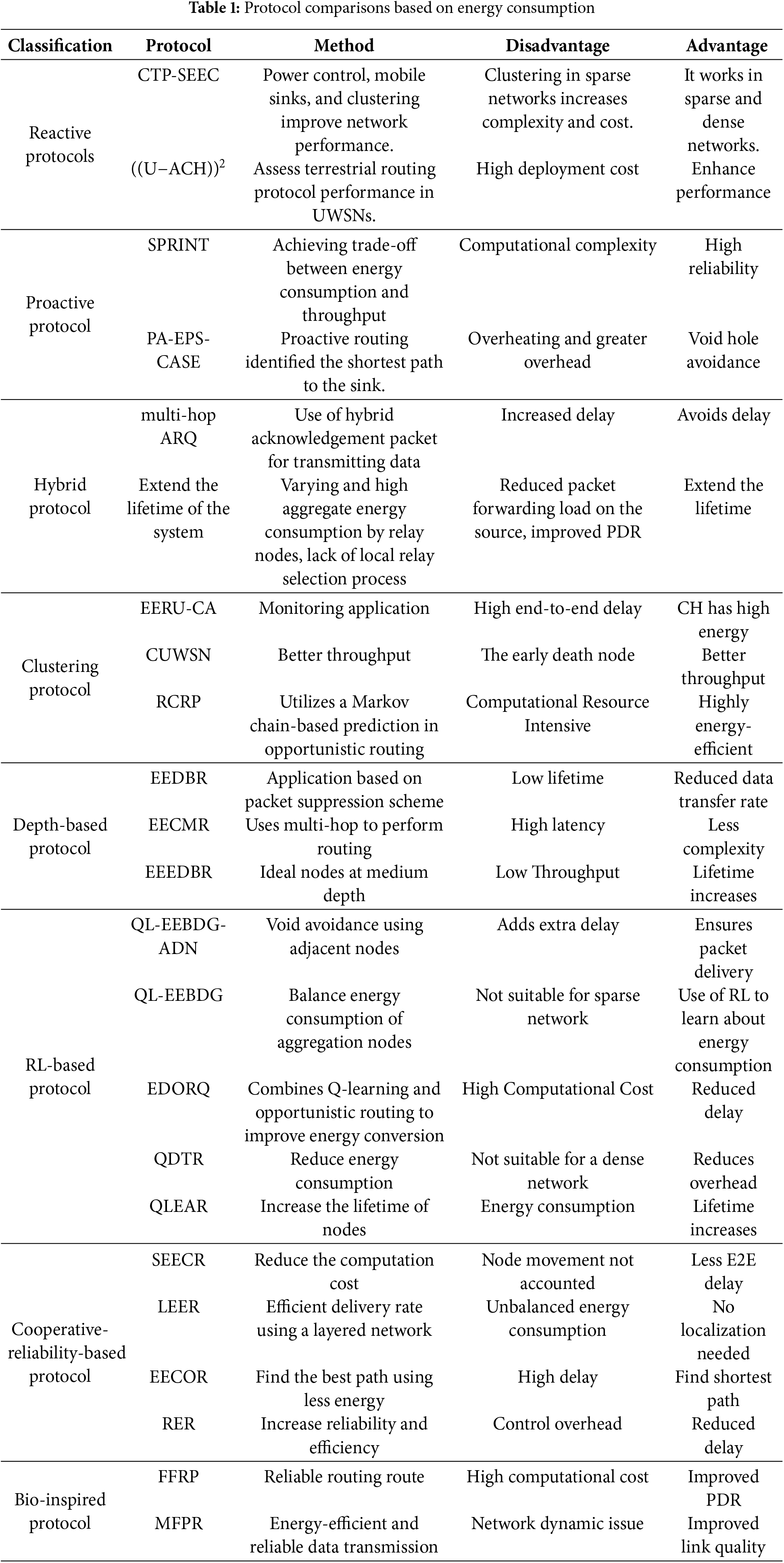
In the network layer, sensors are linked to observers, facilitating data routing and enabling cooperative sensing. To meet the desired levels of energy efficiency, scalability, stability, and convergence in UWSNs, routing protocols must be carefully established. These protocols aim to ensure reliable, energy-efficient paths for nodes while extending the overall network lifespan. Various factors impact the energy consumption of a routing system, such as neighbor discovery, communication processes, and computational demands. Table 1 shows the protocol comparisons based on energy consumption [11,38,52–54].

4.4 Routing Protocols Based on Geographic Information

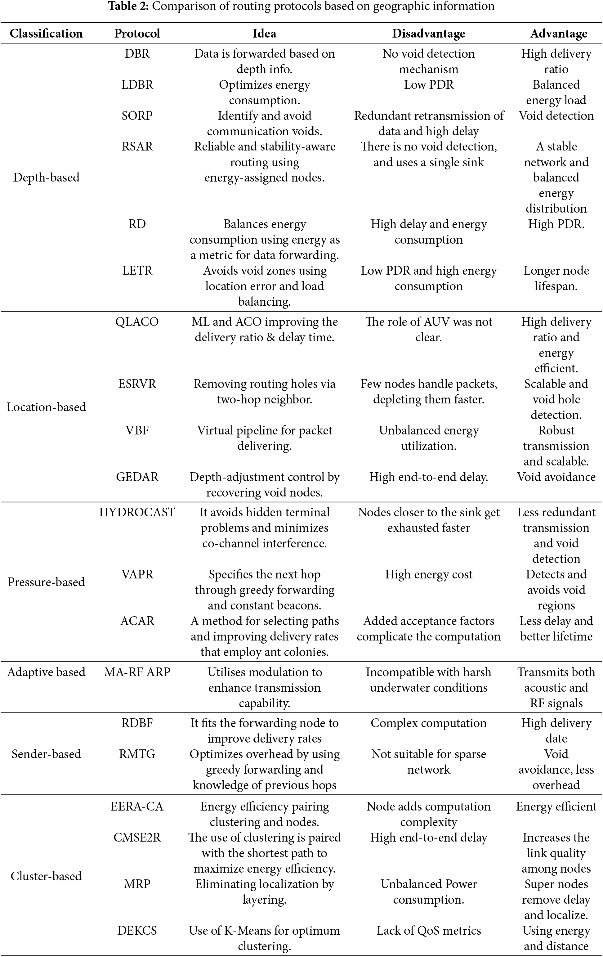
Position-based routing, also referred to as geographic routing, is considered an effective and scalable method for data transmission. Unlike traditional routing approaches, it does not require the establishment or maintenance of an end-to-end path to the destination, nor does it rely on routing messages to update path states. Instead, the routing decisions are made locally at each hop, where the node closest to the destination is selected as the next-hop forwarder. This process continues iteratively until the packet reaches its final destination [7]. A hybrid approach that combines geographic routing with opportunistic routing (OR) enhances data delivery efficiency and reduces energy consumption compared to conventional packet retransmissions [11]. In opportunistic routing, all packets are sent to a list of pre-selected forwarding neighbors ordered by suitability as the next-hop candidate. When the highest-priority node receives the packet successfully, lower-priority nodes abort their scheduled transmissions. When no high-priority node receives the packet, lower-priority nodes proceed and forward, ensuring reliable delivery. Opportunistic routing is highly effective when conventional forwarding methods fail, and it offers an efficient alternative for packet delivery. However, geo-opportunistic routing is susceptible to the communication void region problem. A forwarder node is a void node if it does not have any neighboring nodes that are closer to the destination. When packets arrive at such nodes, routing protocols must perform recovery processes to route packets through empty regions or discard them to prevent unnecessary energy consumption. It is necessary to solve this issue to guarantee the reliability and efficiency of geographic routing methods. Table 2 presents a comparative analysis of routing protocols based on geographic information, highlighting their strengths and limitations [8,55–58].

5  Proposed Algorithm

The proposed network architecture is designed to improve efficiency, scalability, and energy conservation in underwater sensor networks. By reducing waiting times between nodes, data transmission becomes faster and more reliable, which is essential in underwater environments where communication is naturally slow. Additionally, the system enables localized decision-making, allowing each node to analyze its past interactions and adjust its behavior accordingly. This reduces reliance on a central controller, leading to a more adaptive and resilient network. The decentralized approach also enhances scalability, as nodes can function independently without generating excessive control messages, which helps save bandwidth and energy. By minimizing the need for constant coordination, the network remains stable, efficient, and capable of supporting more nodes without performance bottlenecks. Overall, this architecture ensures high throughput, energy efficiency, and scalability, making it well-suited for the challenges of underwater communication.

5.1 Network Model

The network model in this study is designed for a 3D underwater environment, with key assumptions to ensure realistic and efficient operation. Nodes are randomly distributed to reflect practical underwater deployments, and each node starts with predefined energy levels and communication ranges, ensuring a uniform baseline for evaluating energy consumption over time. The model also incorporates standard data transmission rules, including the effects of noise and signal attenuation, to simulate real-world underwater communication challenges. To maintain consistency in performance evaluation, a standard dataset is used to regulate data generation across the network, making results comparable to other studies. Node mobility is kept minimal, simplifying the analysis by focusing on energy consumption and data transmission under near-static conditions. Additionally, each node is equipped with a depth gauge module, allowing it to adjust operations based on its vertical position in the 3D underwater space. These assumptions create a structured and realistic framework for analyzing energy efficiency and communication effectiveness in underwater sensor networks.

5.2 The System Model

This IPv6 distance vector routing protocol works at the physical layer using IEEE 802.15.4, making it suitable for low-power, low-bandwidth sensor networks. Recent advances have improved communication for these networks. This study introduces UWF-RPL, a modified RPL protocol for underwater environments, supporting both stationary and limited-mobility nodes. Significant structural changes were made to adapt RPL for underwater use. Highlights key differences between the proposed UWF-RPL and standard RPL as follows:

•   Rank R(u, j): This metric defines the logical distance of node u, a member of the network set N (u ∈ N), from the root of the network graph J, as calculated by the RPL protocol’s objective function (OF). The rank value R typically increases as the node moves further from the graph’s root. Depending on the specific application, this rank can be determined by the node’s depth relative to the water surface or by combining both step depth and node depth.

•   Destination Oriented Directed Acyclic Graph (DODAG) Preferred Parent (DPP): Let u be a node within the graph G, N(u) its set of one-hop neighbors, and DPP(u,j) a finite subset of N(u). For any neighbor node v in N(u), v will be part of DPP(u,j) if it has the lowest rank relative to the root R(u, j) in the specified DODAG j ∈ B. In the enhanced version of RPL, each node will have multiple preferred parents rather than just one. Node u will select the best parent dynamically based on conditions when sending a packet, ensuring more efficient and reliable data transmission.

•   DODAG Root List (DRL): Every node v ∈ N(u) is required to broadcast DODAG Information Object (DIO) packets, which must include information about the location of the DODAG root. Thus, each node u in the network maintains a root location list, DRL(j), which stores the locations of DODAG roots. This allows nodes to efficiently route data by referencing the root locations stored in their DRL.

•   The parameters we aim to make fuzzy for the proposed system are outlined below:

•   Depth or Vertical Distance: The vertical distance of each sensor node from the water surface plays a critical role in determining communication efficiency and signal strength.

•   Energy Consumption per Communication: The total energy consumed by each node during data transmission influences the network’s overall energy efficiency and the node’s operational lifespan.

•   RSSI/ETX Ratio per Link: The RSSI to ETX ratio for each link helps assess the link quality and reliability between nodes.

•   Packet Latency: The delay encountered during the transmission of each packet or the cumulative latency from the source to the destination, which impacts the speed and efficiency of the data delivery process.

These parameters are crucial for optimizing underwater sensor networks, allowing the system to adapt to dynamic conditions using fuzzy logic. This research employs a triangular cross-layer design, where information is exchanged across different network layers to enhance performance. Given the constraints of underwater environments, integrating RPL with the IEEE 802.15.4 MAC and Physical Layers is essential for improving service quality, link reliability, and energy efficiency. By combining depth, RSSI, energy consumption, and latency into a composite metric, our approach optimizes parent node selection, leading to more efficient and reliable routing. Building on Reference [59], we adapted and refined its concepts for underwater environments, addressing acoustic propagation, dynamic topology, and energy constraints. While the original work focused on terrestrial networks, significant modifications were required for UWSNs. We carefully selected parameters tailored to underwater conditions, ensuring improved routing performance. Sections 5.1 and 5.2 detail the differences in selected metrics and their impact, demonstrating how our approach diverges from Reference [60] to better suit underwater applications.

5.3 Metrics of Interest

This section reviews the key metrics in developing our OF and their impact. Our method improves energy efficiency, selecting routes with low energy consumption to extend network lifespan, incorporating the IEEE 802.15.4 PHY EC parameter. Reliability is ensured by prioritizing a high packet delivery ratio, considering environmental challenges like interference and ocean conditions, and using RSSI and ETX for assessment. Real-time delivery is crucial for applications like accident response and underwater drilling, so latency is included to ensure timely data transmission. The next section presents the mathematical analysis of these metrics.

•   Depth Measurement: Pressure gauges in the underwater sensor network measure the depth of each node based on pressure per unit surface. Depth is calculated by the distance from the water surface, helping nodes adjust their operations accordingly.

•   Energy Consumption: A critical physical layer metric, energy consumption includes both network communication and local CPU processing. The Network Simulator version 2.31 underwater motes datasheet sets the energy range between 0 and 1000 J. Our method calculates total energy consumption along the path to the DODAG root, incorporating both individual and multi-node energy use.

•   Latency Metric: Based on the MAC (Layer 2) link, latency measures the total time needed for a packet to travel from source to destination. It is a cumulative indicator, summing the delays across all nodes on the path. NS2 does not natively measure RPL latency, so we define it based on DIO transmission time from sender to destination. Extensive simulations determine an upper latency bound (n seconds), ensuring realistic performance analysis. This formula is used to calculate the latency factor:

Latency(n)={Latency(P)+Latencyn→P0,Ifnistheroot(14)

In this case, n and P correspond to the node and its parent, respectively. Latency n→P indicates the time delay between nodes n and their parents.

5.4 Fuzzification

This section describes the fuzzy logic architecture, including fuzzification, inference, and defuzzification for selecting the preferred parent node. Our proposed Objective Function (OF) improves underwater RPL performance by combining multiple metrics effectively. Fuzzy logic is a powerful method for integrating different parameters into a single decision-making process. It takes four input metrics—depth, energy consumption, latency, and RSSI/ETX ratio—and processes them to generate a single output: neighbor quality. Fig. 2 illustrates the key steps in the UWF-RPL fuzzy logic design.

Figure 2: The quality of the neighbor output metric (Adapted from [59])

5.4.1 Procedure for Fuzzification

In fuzzification, numerical input variables are allocated to fuzzy sets with some membership level. A description of the fuzzification technique is provided in the following subsections, including the identification of linguistic variables and membership functions for each metric.

5.4.2 Homogenization or Normalization of Variables

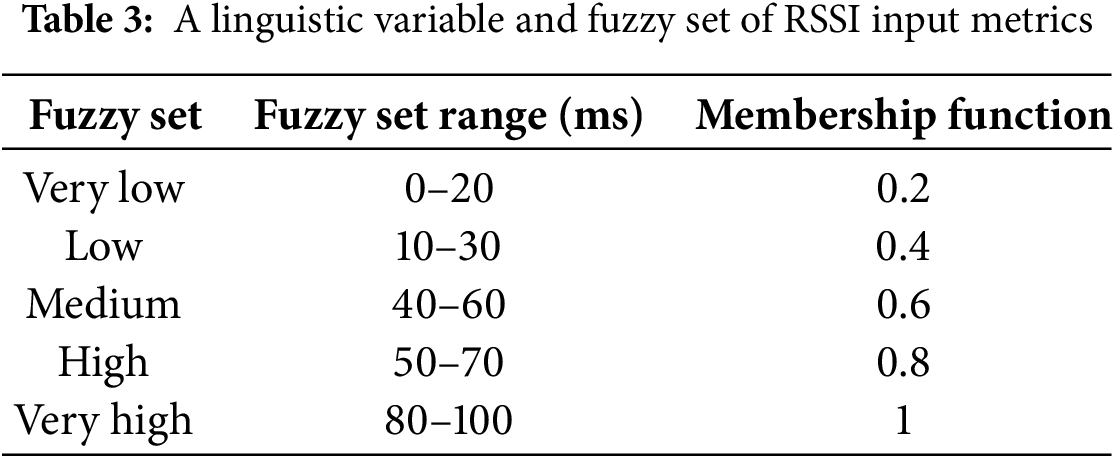
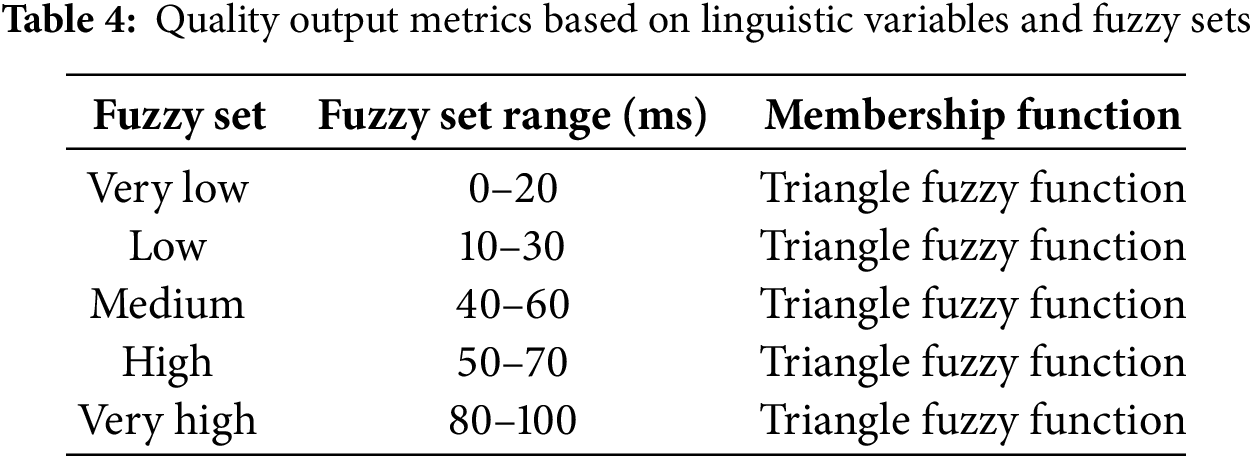
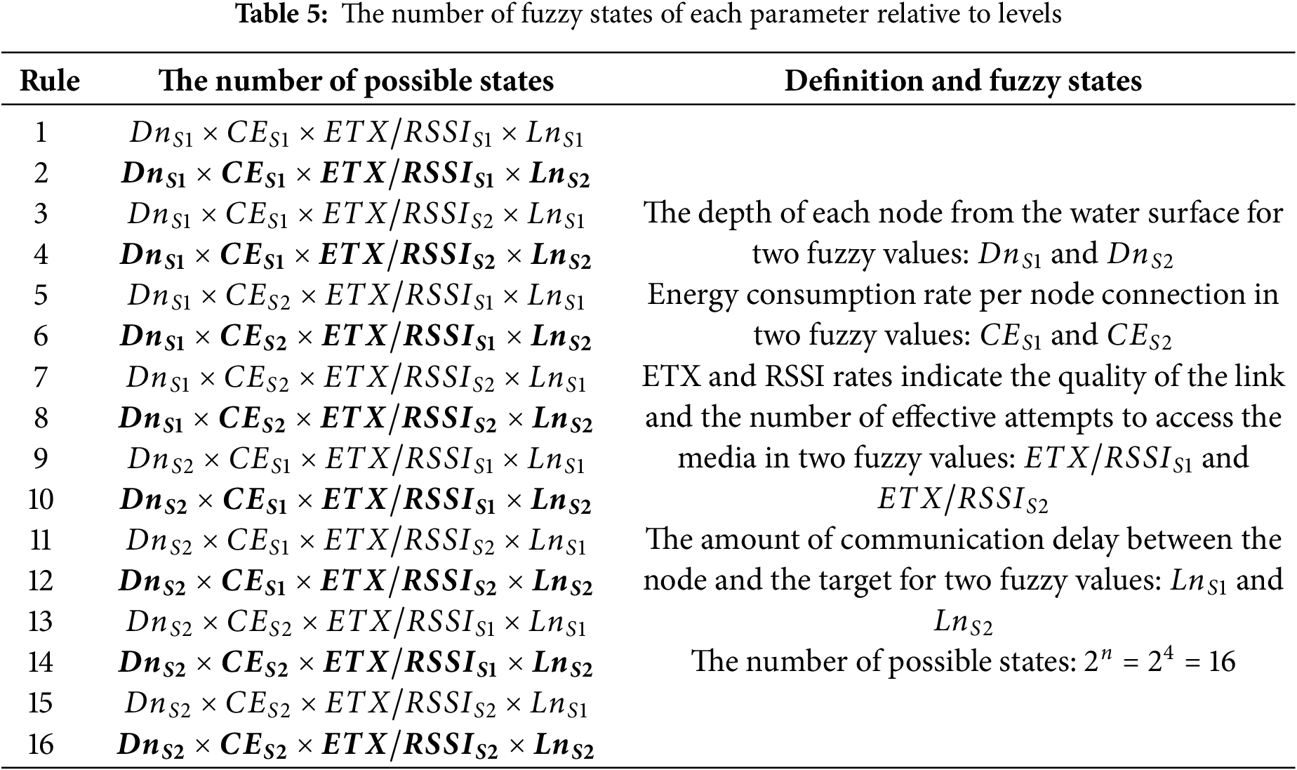
In Fuzzy systems, rather than numbers, the values of the linguistic variable are words. There are three fuzzy sets for each input metric in the UWF-RPL’s OF, while eight are for each output variable. In addition, the following details are provided. Fuzzifying the X input variable. The fuzzy sets of metrics input metrics have five linguistic names, “Very Low”, “Low”, “Medium”, “High”, and “Very High”. Table 3 presents the fuzzy sets along with their ranges, besides the membership function of this metric. Enhancing the quality of neighbor output variables by fuzzing. There are eight fuzzy sets of linguistic names for the quality of neighbor output.

These metrics are in Tables 4 and 5 as fuzzy sets, their ranges, and their membership functions.

5.4.3 The Membership Functions

A fuzzy set is visually represented using a membership function, which assigns values between 0 and 1 to indicate the degree of belonging. The choice of a membership function depends on several factors, such as trial-and-error simulations, previous research, specific application needs, and device datasheets. Since trapezoidal functions are widely used in fuzzy logic, we selected them as input metrics for our design [59]. Aside from the Trapezoidal process, two special functions, R- and L-functions, are derived from it [60–62].

5.4.4 System of Fuzzy Inferences

These subsections explain the procedures for evaluating rules based on fuzzy sets and aggregating rules using the Mamdani inference system and how rules are evaluated in Section 5.4.5. In the following, we introduce the rule evaluation. (A fuzzy logic rule is constructed at this stage using IF-THEN conditions (i.e., rules of the form “If condition, then result”). According to the UWF-RPL’s OF, the number of generated rules depends on the number of input metrics and fuzzy sets associated with each metric).

5.4.5 Fuzzy Base Rules

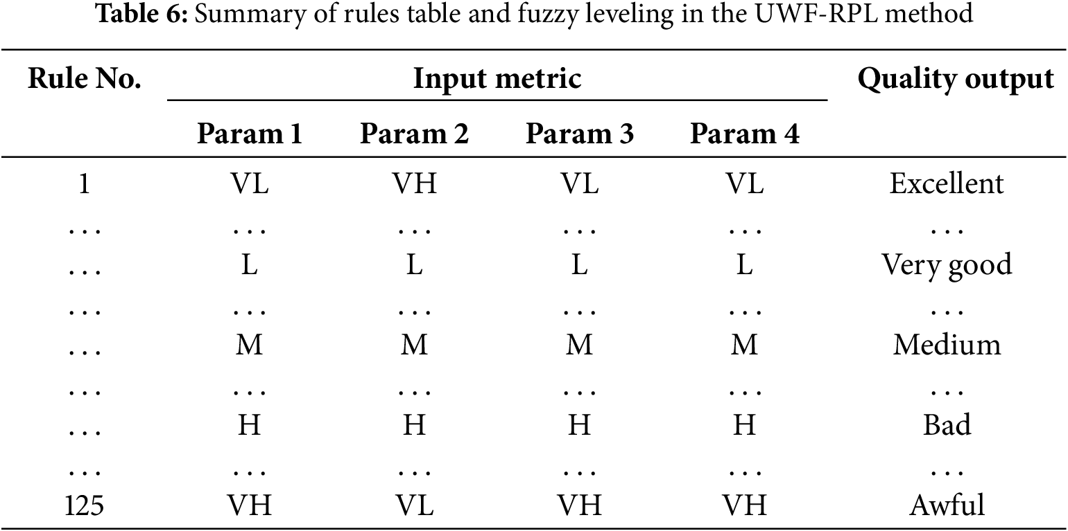
In the fuzzy system, we have applied the Mamdani leveling method, ensuring that each specific situation is assigned a corresponding fuzzy value for that level. While some results may appear similar due to the closeness of levels, combining all factors in the fuzzy output effectively resolves these similarity percentages, ensuring distinct and accurate outcomes (Table 6).

5.4.6 Membership Fuzzy

Our research uses the Mamdani inference system for fuzzy logic decision-making, combining rule outputs through fuzzy aggregation. We apply “AND” (Minimum) and “OR” (Maximum) operators to determine how rules are integrated into the final decision. The “Maximum” operator prioritizes the most influential rule, ensuring accurate outcomes. In our design, five out of eleven possible rules are triggered to determine the “Average” fuzzy output quality. A formula calculates this quality based on the number of activated rules and their contributions. This flexible approach allows the system to adapt dynamically, improving decision-making even when only a subset of rules is applied, enhancing overall fuzzy logic performance.

Average=Max(Min(FarDn,CE,ETX&RSSI, and longLn),Min(NearDn,CE,ETX&RSSI,and ShortLn)Min(CloseDn,CE,ETX&RSSI, and longLn), Min(NearDn,CE,ETX&RSSI, and AverageLn),)(15)

5.4.7 Defuzzification Process

Optimizing the fitness function is necessary to improve the efficiency of the network and reduce congestion.

NCn=(∑i=116Ui×wj)/(∑i=116Ui)(16)

Fitness Function(fi)=Max(1min(∑i=116((w1×Di)+(w2×CEi)+(w3×ETX&RSSi)+(w4×Lni))∑i=116Ui)(17)

where i is the number of fuzzy rules ranging from 1 to 16 (based on Table 5). And w1, w2, w3, w4 are the weights of each state on the algorithm and fuzzy calculations.

5.4.8 Selecting Parent

This section explains how UWF-RPL constructs a DODAG allowing nodes to choose a preferred parent for data transmission. The DODAG root (sink node) collects network data and distributes DIO messages to inform nodes about the network structure. Nodes within range process this information and decide whether to join the DODAG based on its attributes. Each RPL instance can contain multiple DODAGs, each with a unique identifier assigned by the root as an 8-bit value. A node can join only one DODAG per instance, but all DODAGs in the same instance use the same Objective Function (OF). The DODAG root also assigns IPv6 addresses for identification. When a new DODAG version is created, the version number is updated at the root (Fig. 3).

Figure 3: The process of node’s parent selection

An increase in the DODAG version number signals a global repair process at the root, releasing a new version to fix loop detection and link failures. Local repairs try to resolve issues without rebuilding the entire DODAG, but if unsuccessful, global repair is needed. Each DODAG version is identified by a unique ID, consisting of the RPL instance identifier, DODAG identifier, and version number. The root sends a DIO message to neighbors, which verify its authenticity using the DODAG version and parent ID before adding the sender to their parent list. Network stability improves when DIO message frequency decreases, but in unstable conditions, the interval is minimized, maximizing DIO transmissions. The DIO message contains an OCP (Objective Code Point), a 16-bit identifier for selecting the appropriate Objective Function (OF). Existing OFs use single or multiple criteria, while our research introduces a new OF based on fuzzy logic. The fuzzification step determines membership functions for each input, forming the basis of our fuzzy logic design.

5.5 Queue Management Phase

In the second phase of the proposed protocol, after the network graph is formed and data is transferred to the root, the network state changes due to bottlenecks, traffic fluctuations, and queue status. The standard RPL method lacks mechanisms to manage node direction, control congestion, or prevent queue overflow. To address this, our approach estimates and prevents bottlenecks at parent nodes, particularly those near the sink. Our method monitors incoming and outgoing packets at parent nodes, modeling this process using Eq. (18). When a queue reaches a critical threshold, the parent notifies child nodes via a beacon, the smallest control message. Based on this signal, child nodes can either continue sending data, pause transmission or resume once congestion reduces.

A third option is switching to a new parent, but this increases network overhead. If a node itself is congested, its children must adjust their sending rates instead. The queue indicator, calculated using Eq. (18), helps manage this process efficiently.

QueueState={(λΔtμΔt)≤1(λΔtμΔt)>1(18)

In this context, λΔt represents the rate at which packets enter the node’s queue, while μΔt signifies the rate at which packets leave the queue. In the first scenario, when the entry rate is lower than the exit rate, the probability of congestion is low. In the second scenario, the likelihood of congestion increases when the entry rate exceeds the exit rate. The difference between these rates, λΔt−μΔt, plays a critical role in determining the node’s behavior. If the difference between the entry and exit rates is smaller than the remaining slots in the queue, the node will refrain from sending a beacon message. However, if the difference exceeds the number of available slots in the queue, the node will send a beacon to reduce incoming traffic by half. Should the queue overflow again, the node will broadcast another beacon to its neighboring nodes, requesting an additional 50% reduction in traffic. This stepwise reduction typically results in a total traffic decrease of around 75%, as illustrated in Fig. 4.

Figure 4: The process of Queue management

6  Evaluation and Comparison

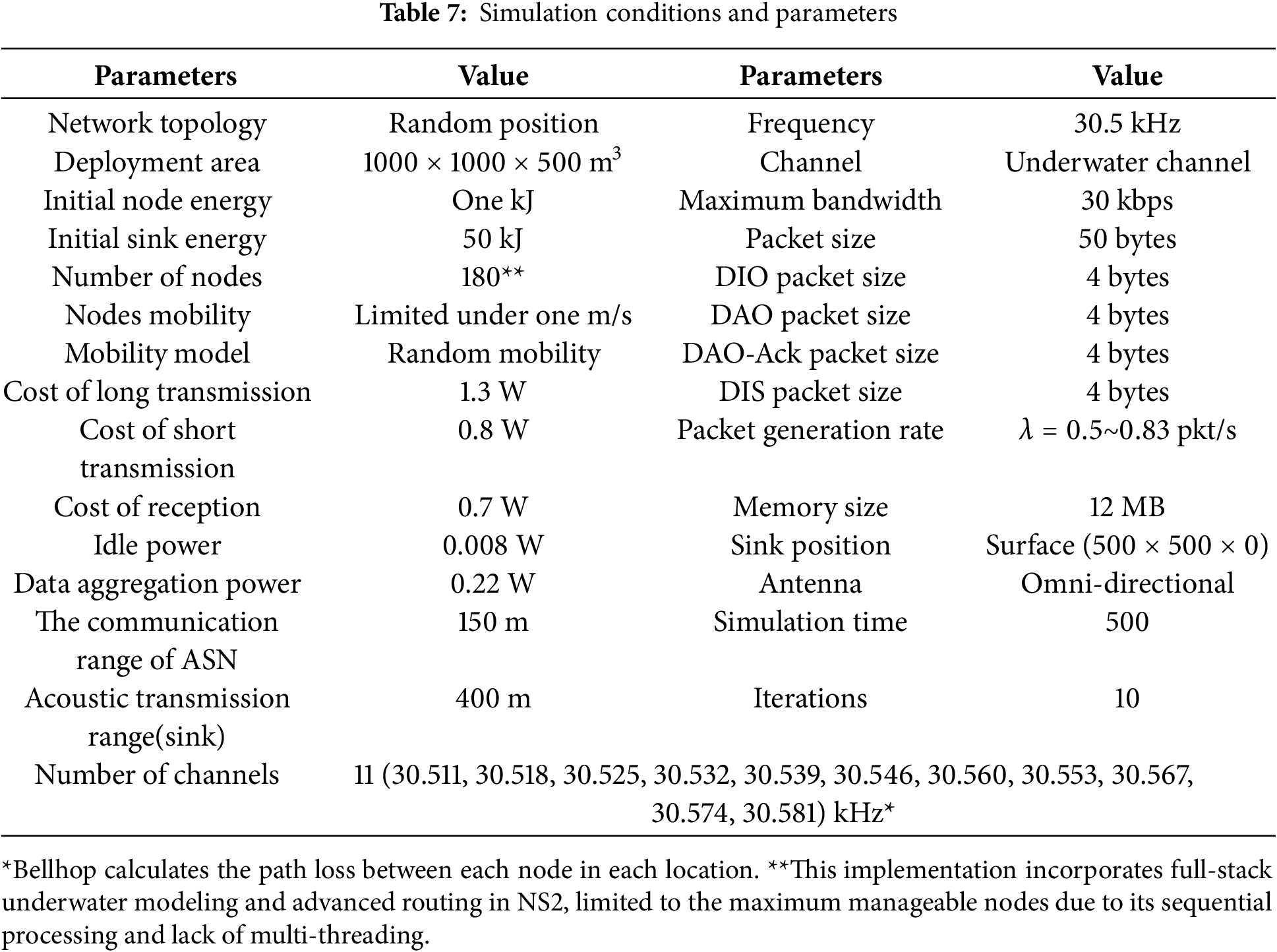
In this section, we expand our evaluation to include comparisons of the UWF-RPL method with traditional RPL, the Distance and Energy constrained K-means Clustering Scheme (DEKCS) method from 2022, and the newly integrated Reliable Cluster Based Routing Protocol (RCRP) from 2024. Our simulations, conducted in NS version 2.31 with the Aquasim package, adjust the basic RPL model for the underwater environment by shifting from magnetic to acoustic channels and revising all network layers for optimal underwater functionality. The UWF-RPL method enhances the basic RPL’s Objective Function to improve parent selection criteria, while RCRP introduces a cluster-based and opportunistic routing strategy, tailored to manage the dynamic nature and energy constraints of underwater networks. Our analysis focuses on key performance metrics such as network convergence time, the number of surviving nodes, packet delivery ratio, delay per hop, energy consumption, and network overhead, providing a comprehensive view of each method’s effectiveness in the simulated underwater conditions (Table 7).

6.1 Network Convergence Time Test

This test lasts when the network is formed; in other words, the network graph is created, and the nodes are ready to send packets to the well. To perform this test, we considered the network traffic and data production rate at two values of 30 and 50 packets per minute to measure efficiency in the quiet and busy traffic environment. The convergence time criteria will change during the simulation time because network nodes may be lost, and local repairs are required. In the UWF-RPL network, fuzzy calculations are performed in each node and periodically sent to the neighbors by the DIO message in the RPL structure.

As a result, no additional overhead is imposed on the network. To calculate this time, cumulatively sampled in time units every 25 s, the duration of local and global convergence is aggregated in the network. As expected, the UWF-RPL method in this test has performed better than the other two methods point-wise and, finally, on average. Fig. 5 shows the timing diagram of local and global convergences. In this test, due to the instability of RPL, DEKCS, and RCRP methods, a difference of about 10%–23% is observed. The higher the number of instabilities on the network, the worse the results will be. Fig. 6 shows the average graph of this convergence time for three protocols in two modes with transmission densities of 30 and 50 packets per minute.

Figure 5: Convergence time of network nodes in 500 s and with two traffics of 30 and 50 pkt/m

Figure 6: The average convergence time of network nodes with two traffic rates of 30 and 50 pkt/m

6.2 Testing the Number of Live Network Nodes

In the underwater sensor network, it is evident that the aggregation and exchange of packets consume energy with the passage of time and the activity of network nodes. If a node has exhausted its battery energy, it is removed from the network. Nodes consume energy for each of their internal and network activities (Fig. 7). Even though the network nodes may not be necessary at the edges of the graph when they appear as routers or aggregators, their death can harm the system’s performance.

Figure 7: Number of live network nodes during 500 s simulations

Therefore, we can expect to see a postponement of the death time of the nodes as the energy consumption rate is distributed throughout the network. Based on a fuzzy OF, the UWF-RPL method selects the next step in the network based on the fuzzy value of the neighboring node. If the node does not have the desired value, it is separated from the parent list of children by agreement and acts as a leaf node until its neighbors have reached the same level. As part of the OF of this case, the network nodes need to interact more in this process, and the control overhead is considerably less than the control overhead incurred by the early death of network nodes or messages from parentless children.

6.3 Packet Delivery Rate Test

Another important factor in wireless networks’ qualitative and quantitative assessment is their ability to deliver network packets to their destinations. The number of attempts to transfer and the percentage of successful transfers are considered in this test. This criterion directly relates to route control, flow rate, and the number of active routes in front of network trace nodes. It is possible to achieve a higher delivery rate when network flows are more distributed. It is important to note that the shortest path is sometimes the best. In our UWF-RPL fuzzy method, delay measures, ETX rate, and RSSI are critical players in reducing collisions and packet failures. In the UWF-RPL method, a combination of these metrics and queue management has been included in the decisions of the nodes to select the parent.

Simulation results show that the UWF-RPL method achieves packet delivery rates of 91%–73% in low-density networks and 86%–64% in high-density networks. On average, the UWF-RPL approach maintains an 84% delivery rate for low traffic and 76% for high traffic. In comparison, the base RPL method achieves 68% and 60%, the DEKCS method reaches 78% and 73%, and the RPRC method attains 81% and 70%, respectively (Fig. 8).

Figure 8: The delivery rate is low and high-traffic environments during 500 s simulation

6.4 Delay per Hop Test

Network latency is defined by the average end-to-end packet transmission delay time. Therefore, the network’s delay parameter depends on the number of steps a packet takes to reach its destination. According to the definition of overall delay caused by processing, it is queuing, transmission, and propagation.

The more steps between the source and destination of a packet, the more cumulative the end-to-end delay rate increases. On the other hand, due to the funnel effect in the network, the packet delay rate in the lower layers close to the leaves is lower due to the lack of density and crowding, and the closer we get to the root, the more likely the collision and funnel effect will be. This test measured the average end-to-end delay rate of network packets in steps between 1 and 4 (Figs. 9–11).

Figure 9: Evaluation of UWF-RPL network for the traffic of 30 packets per minute

Figure 10: Evaluation of UWF-RPL network for the traffic of 50 packets per minute

Figure 11: The average delay concerning the number of steps per traffic of 30 and 50 packets per minute

6.5 Network Energy Consumption Test

In underwater sensor networks, node batteries cannot be recharged, making energy consumption a critical factor. A slower decline in energy indicates better energy management by the protocol. This test examines the relationship between remaining nodes and time, as network lifetime depends on how long individual nodes remain active. The network’s lifetime is measured until the first node dies. In static sink networks, nodes near the sink drain energy faster due to higher relay workloads, eventually disconnecting the sink—a process called sink encirclement. Since recharging or replacing nodes is nearly impossible, monitoring network lifespan is essential. This test tracks the decrease in live nodes over rounds, considering node position and remaining energy to assess stability and energy consumption trends as per Figs. 12 and 13.

Figure 12: Network energy consumption rate in 500 s of simulation

Figure 13: The total energy consumed after 500 s of simulation

6.6 Overhead Control Packets

This parameter evaluates how well UWF-RPL establishes a path and delivers packets from the source to the destination. In simulations, UWF-RPL and the baseline method were compared by analyzing the number of sent and received packets, measuring the protocol’s ability to safely transmit data. To transfer these packets, control messages such as DIO, DAO, and Destination Advertisement Object Acknowledgement (DAO-Ack) are required. While UWF-RPL still uses these messages, their content and transmission frequency have been optimized, reducing control packet overhead. Since network node distribution is random in simulations, results vary across runs. However, UWF-RPL consistently outperforms the baseline method, as shown in Fig. 14.

Figure 14: Chart of control message rate in 500 s of simulation

7  Conclusion

The proposed UWF-RPL protocol employs a multi-metric, fuzzy-based parent-selection process and an adaptive queue-management strategy to tackle major constraints in underwater wireless sensor networks, such as high propagation delays, bandwidth limitations, and stringent energy requirements. By incorporating depth, residual energy, link quality (RSSI/ETX), and latency into its decision-making mechanism, UWF-RPL optimally balances data forwarding across the network, reduces queue overflow, and extends the operational lifetime of sensor nodes. The result justifies the possibility of improving RPL, DEKCS, and RCRP in packet delivery, convergence time, and energy consumption to ensure efficient and robust network performance. Our future research will focus on integrating machine learning methods, in particular deep reinforcement learning to enhance routing decisions and predict bottlenecks. Researchers can also study new underwater sensing technologies with multimode sensing capabilities e.g., hybrid acoustic-optical nodes to enhance data capture fidelity and reduce overhead in communication. Finally, real-world testing of UWF-RPL at a large scale and synchronization with autonomous underwater vehicles would provide further evidence of its resilience and scalability and make the protocol practical for several underwater applications.

Acknowledgement: Not applicable.

Funding Statement: The authors received no specific funding for this study.

Author Contributions: The authors confirm contribution to the paper as follows: Study conception and design: Mehran Tarif, Mohammadhossein Homaei; Data collection: Mohammadhossein Homaei; Analysis and interpretation of results: Mehran Tarif, Mohammadhossein Homaei, Amir Mosavi; Draft manuscript preparation: Mohammadhossein Homaei, Amir Mosavi; Final approval: All authors. All authors reviewed the results and approved the final version of the manuscript.

Availability of Data and Materials: The datasets generated and/or analyzed during the current study are available from the corresponding author on reasonable request.

Ethics Approval: Not applicable.

Conflicts of Interest: The authors declare no conflicts of interest to report regarding the present study.

References

1. Bello O, Zeadally S. Internet of underwater things communication: architecture, technologies, research challenges and future opportunities. Ad Hoc Netw. 2022;135(6):102933. doi:10.1016/j.adhoc.2022.102933. [Google Scholar] [CrossRef]

2. Nkenyereye L, Nkenyereye L, Ndibanje B. Internet of underwater things: a survey on simulation tools and 5G-based underwater networks. Electronics. 2024;13(3):474. doi:10.3390/electronics13030474. [Google Scholar] [CrossRef]

3. Khan ZU, Gang Q, Muhammad A, Muzzammil M, Khan SU, Affendi MEI, et al. A comprehensive survey of energy-efficient mac and routing protocols for underwater wireless sensor networks. Electronics. 2022;11(19):3015. doi:10.3390/electronics11193015. [Google Scholar] [CrossRef]

4. Ali ES, Saeed RA, Eltahir IK, Khalifa OO. A systematic review on energy efficiency in the internet of underwater things (IoUTrecent approaches and research gaps. J Netw Comput Appl. 2023;213(3):103594. doi:10.1016/j.jnca.2023.103594. [Google Scholar] [CrossRef]

5. Qiu T, Li Y, Feng X. Distributed channel sensing MAC protocol for multi-UUV underwater acoustic network. IEEE Internet Things J. 2024;11(9):16119–33. doi:10.1109/JIOT.2024.3352007. [Google Scholar] [CrossRef]

6. Mohsan SAH, Li Y, Sadiq M, Liang J, Khan MA. Recent advances, future trends, applications and challenges of internet of underwater things (IoUTa comprehensive review. J Mar Sci Eng. 2023;11(1):124. doi:10.3390/jmse11010124. [Google Scholar] [CrossRef]

7. Shovon II, Shin S. Survey on multi-path routing protocols of underwater wireless sensor networks: advancement and applications. Electronics. 2022;11(21):3467. doi:10.3390/electronics11213467. [Google Scholar] [CrossRef]

8. Ismail AS, Wang X, Hawbani A, Alsamhi S, Abdel AS. Routing protocols classification for underwater wireless sensor networks based on localization and mobility. Wirel Netw. 2022;28(2):797–826. doi:10.1007/s11276-021-02880-z. [Google Scholar] [CrossRef]

9. Datta A, Dasgupta M. Time synchronization in underwater wireless sensor networks: a survey. In: Proceedings of the Seventh International Conference on Mathematics and Computing; 2022 Feb 21–24; London, UK. p. 427–37. [Google Scholar]

10. Tarif M, Moghadam BN. A review of energy efficient routing protocols in underwater internet of things. arXiv:231211725. 2023. [Google Scholar]

11. Menon VG, Midhunchakkaravarthy D, Sujith A, John S, Li X, Khosravi MR. Towards energy-efficient and delay-optimized opportunistic routing in underwater acoustic sensor networks for IoUT platforms: an overview and new suggestions. Comput Intell Neurosci. 2022;2022(1):7061617. doi:10.1155/2022/7061617. [Google Scholar] [PubMed] [CrossRef]

12. Islam KY, Ahmad I, Habibi D, Waqar A. A survey on energy efficiency in underwater wireless communications. J Netw Comput Appl. 2022;198(7):103295. doi:10.1016/j.jnca.2021.103295. [Google Scholar] [CrossRef]

13. Mohsan SAH, Mazinani A, Othman NQH, Amjad H. Towards the internet of underwater things: a comprehensive survey. Earth Sci Inform. 2022;15(2):735–64. doi:10.1007/s12145-021-00762-8. [Google Scholar] [CrossRef]

14. Dai M, Li Y, Li P, Wu Y, Qian L, Lin B, et al. A survey on integrated sensing, communication, and computing networks for smart oceans. J Sens Actuator Netw. 2022;11(4):70. doi:10.3390/jsan11040070. [Google Scholar] [CrossRef]

15. Dhongdi SC. Review of underwater mobile sensor network for ocean phenomena monitoring. J Netw Comput Appl. 2022;205(3):103418. doi:10.1016/j.jnca.2022.103418. [Google Scholar] [CrossRef]

16. Ragavi B, Baranidharan V, John CSA, Pavithra L, Gokulraju S. A comprehensive survey on different routing protocols and challenges in underwater acoustic sensor networks. In: Yadav S, Chaudhary KP, Gahlot A, Arya Y, Dahiya A, Garg N, editors. Recent advances in metrology. Berlin/Heidelberg, Germany: Springer; 2023. p. 309–20. [Google Scholar]

17. Ali MA, Mohideen SK, Vedachalam N. Current status of underwater wireless communication techniques: a review. In: 2022 Second International Conference on Advances in Electrical, Computing, Communication and Sustainable Technologies (ICAECT); 2022 Apr 21–22; Bhilai, India. p. 1–9. [Google Scholar]

18. Homaei MH, Salwana E, Shamshirband S. An enhanced distributed data aggregation method in the internet of things. Sensors. 2019;19(14):3173. doi:10.3390/s19143173. [Google Scholar] [PubMed] [CrossRef]

19. Mei H, Wang H, Shen X, Jiang Z, Yan Y, Sun L, et al. Node load and location-based clustering protocol for underwater acoustic sensor networks. J Mar Sci Eng. 2024;12(6):982. doi:10.3390/jmse12060982. [Google Scholar] [CrossRef]

20. Kumar M, Goyal N, Singh AK, Kumar R, Rana AK. Analysis and performance evaluation of computation models for node localization in deep sea using UWSN. Int J Commun Syst. 2024;37(11):1–23. doi:10.1002/dac.5798. [Google Scholar] [CrossRef]

21. Nanthakumar S, Jothilakshmi P. A comparative study of range based and range free algorithm for node localization in underwater. E-Prime-Adv Electr Eng Electron Energy. 2024;9(7):100727. doi:10.1016/j.prime.2024.100727. [Google Scholar] [CrossRef]

22. Omari M, Kaddi M, Salameh K, Alnoman A, Elfatmi K, Baarab F. Enhancing node localization accuracy in wireless sensor networks: a hybrid approach leveraging bounding box and harmony search. IEEE Access. 2024;12(3):86752–81. doi:10.1109/ACCESS.2024.3417227. [Google Scholar] [CrossRef]

23. Abdulhussein AS, Al-Qurabat KM. Exploring radio frequency-based UAV localization techniques: a comprehensive review. Int J Comput Digit Syst. 2024;15(1):1565–81. doi:10.12785/ijcds/1501111. [Google Scholar] [CrossRef]

24. Gola KK. A comprehensive survey of localization schemes and routing protocols with fault tolerant mechanism in UWSN-Recent progress and future prospects. Multimed Tools Appl. 2024;83(31):76449–503. doi:10.1007/s11042-024-18525-0. [Google Scholar] [CrossRef]

25. Wei X, Guo H, Wang X, Wang X, Qiu M. Reliable data collection techniques in underwater wireless sensor networks: a survey. IEEE Commun Surv Tutor. 2022;24(1):404–31. doi:10.1109/COMST.2021.3134955. [Google Scholar] [CrossRef]

26. Gupta O, Goyal N. The evolution of data gathering static and mobility models in underwater wireless sensor networks: a survey. J Ambient Intell Humaniz Comput. 2021;12(10):9757–73. doi:10.1007/s12652-020-02719-z. [Google Scholar] [CrossRef]

27. Ghanem M, Mansoor AM, Ahmad R. A systematic literature review on mobility in terrestrial and underwater wireless sensor networks. Int J Commun Syst. 2021;34(10):e4799. doi:10.1002/dac.4799. [Google Scholar] [CrossRef]

28. Choudhary M, Goyal N. Data collection routing techniques in underwater wireless sensor networks. In: 2021 9th International Conference on Reliability, Infocom Technologies and Optimization (Trends and Future Directions) (ICRITO); 2021 Sep 3–4; Noida, India. p. 1–6. [Google Scholar]

29. Sandhiyaa S, Gomathy C. A Survey on underwater wireless sensor networks: challenges, requirements, and opportunities. In: 2021 Fifth International Conference on I-SMAC (IoT in Social, Mobile, Analytics and Cloud) (I-SMAC); 2021 Nov 11–13; Palladam, India. p. 1417–27. [Google Scholar]

30. Gupta O, Goyal N, Anand D, Kadry S, Nam Y, Singh A. Underwater networked wireless sensor data collection for computational intelligence techniques: issues, challenges, and approaches. IEEE Access. 2020;8:122959–74. doi:10.1109/ACCESS.2020.3007502. [Google Scholar] [PubMed] [CrossRef]

31. Ding J, Wang C, Jiang M, Lin S, Yang H. Cross media routing and clustering algorithm for autonomous marine systems. In: 2021 4th IEEE International Conference on Industrial Cyber-Physical Systems (ICPS); 2021 May 10–12; Victoria, BC, Canada. p. 289–96. [Google Scholar]

32. Rajasekaran L, Santhanam SM. Optimum frequency selection for localization of underwater AUV using dynamic positioning parameters. Microsyst Technol. 2021;27(12):4291–303. doi:10.1007/s00542-021-05222-3. [Google Scholar] [CrossRef]

33. Nazareth P, Chandavarkar BR. Void-aware routing protocols for underwater communication networks: a survey. Evol Comput Mob Sustain Netw. 2021;53:747–60. doi:10.1007/978-981-15-5258-8. [Google Scholar] [CrossRef]

34. Pal A, Campagnaro F, Ashraf K, Rahman MR, Ashok A, Guo H. Communication for underwater sensor networks: a comprehensive summary. ACM Trans Sens Netw. 2022;19(1):1–44. doi:10.1145/3546827. [Google Scholar] [CrossRef]

35. Zhang S, Yang Y, Xu T, Qin X, Liu Y. Long-range LBL underwater acoustic navigation considering Earth curvature and Doppler effect. Measurement. 2025;240:115524. doi:10.1016/j.measurement.2024.115524. [Google Scholar] [CrossRef]

36. Gupta S, Singh NP. Underwater wireless sensor networks: a review of routing protocols, taxonomy, and future directions. J Supercomput. 2024;80(4):5163–96. doi:10.1007/s11227-023-05646-w. [Google Scholar] [CrossRef]

37. Homaei M. Low energy adaptive clustering hierarchy protocol (LEACH). [cited 2025 Jan 1]. Available from: https://www.mathworks.com/matlabcentral/fileexchange/44073-low-energy-adaptive-clustering-hierarchy-protocol-leach. [Google Scholar]

38. Datta A, Dasgupta M. Energy efficient layered cluster head rotation based routing protocol for underwater wireless sensor networks. Wirel Pers Commun. 2022;125(3):2497–514. doi:10.1007/s11277-022-09671-5. [Google Scholar] [CrossRef]

39. Gite P, Shrivastava A, Krishna KM, Kusumadevi GH, Dilip R, Potdar RM. Under water motion tracking and monitoring using wireless sensor network and machine learning. Mater Today Proc. 2023;80(3):3511–6. doi:10.1016/j.matpr.2021.07.283. [Google Scholar] [CrossRef]

40. Sathish K, Venkata RC, Anbazhagan R, Pau G. Review of localization and clustering in USV and AUV for underwater wireless sensor networks. Telecom. 2023;4(1):43–64. doi:10.3390/telecom4010004. [Google Scholar] [CrossRef]

41. Liu Y, Wang H, Cai L, Shen X, Zhao R. Fundamentals and advancements of topology discovery in underwater acoustic sensor networks: a review. IEEE Sensors J. 2021;21(19):21159–74. doi:10.1109/JSEN.2021.3104533. [Google Scholar] [CrossRef]

42. Kulla E, Matsuo K, Barolli L. MAC layer protocols for underwater acoustic sensor networks: a survey. In: International Conference on Innovative Mobile and Internet Services in Ubiquitous Computing; 2022 Jun 29–Jul 1; Kitakyushu, Japan. p. 211–20. [Google Scholar]

43. Sun K, Cui W, Chen C. Review of underwater sensing technologies and applications. Sensors. 2021;21(23):7849. doi:10.3390/s21237849. [Google Scholar] [PubMed] [CrossRef]

44. Amoroso PP, Parente C. The importance of sound velocity determination for bathymetric survey. Acta IMEKO. 2021;10(4):46–53. doi:10.21014/acta_imeko.v10i4.1120. [Google Scholar] [CrossRef]

45. Kumara S, Vatsb C. Underwater communication: a detailed review. In: CEUR Workshop Proceedings; 2021 Oct 4–5; Naples, Italy. [Google Scholar]

46. Niu Q, Zhang Q, Shi W. Waveform design and signal processing method for integrated underwater detection and communication system. IET Radar Sonar Navig. 2023;17(4):617–27. doi:10.1049/rsn2.12365. [Google Scholar] [CrossRef]

47. Sathish K, Hamdi M, Chinthaginjala VR, Alibakhshikenari M, Ayadi M, Pau G, et al. Acoustic wave reflection in water affects underwater wireless sensor networks. Sensors. 2023;23(11):5108. doi:10.3390/s23115108. [Google Scholar] [PubMed] [CrossRef]

48. Huang F, Zhang Y, Guo Q, Tao J, Zakharov Y, Wang B. A robust iterative receiver for single carrier under-water acoustic communications under impulsive noise. Appl Acoust. 2023;210(1):109438. doi:10.1016/j.apacoust.2023.109438. [Google Scholar] [CrossRef]

49. Wang J, Zhou M, Cui Y, Sun H, Han G. Underwater acoustic noise modeling based on generative-adversarial-network. In: Lyu Z, editor. Applications of generative AI. Berlin/Heidelberg, Germany: Springer; 2024. p. 351–69. [Google Scholar]

50. Luo J, Yang Y, Wang Z, Chen Y. Localization algorithm for underwater sensor network: a review. IEEE-Ternet Things J. 2021;8(17):13126–44. doi:10.1109/JIOT.2021.3081918. [Google Scholar] [CrossRef]

51. Menaka D, Gauni S. An energy efficient dead reckoning localization for mobile Underwater Acoustic Sensor Networks. Sustain Comput Inform Syst. 2022;36(3):100808. doi:10.1016/j.suscom.2022.100808. [Google Scholar] [CrossRef]

52. Hayder IA, Khan SN, Althobiani F, Irfan M, Idrees M, Ullah S, et al. Towards controlled transmission: a novel power-based sparsity-aware and energy-efficient clustering for underwater sensor networks in marine transport safety. Electronics. 2021;10(7):854. doi:10.3390/electronics10070854. [Google Scholar] [CrossRef]

53. Khisa S, Moh S. Survey on recent advancements in energy-efficient routing protocols for underwater wireless sensor networks. IEEE Access. 2021;9:55045–62. doi:10.1109/ACCESS.2021.3071490. [Google Scholar] [CrossRef]

54. Zhu R, Boukerche A, Chen Y, Yang Q. A reliable cluster-based opportunistic routing protocol for underwater wireless sensor networks. Comput Netw. 2024;251(1):110622. doi:10.1016/j.comnet.2024.110622. [Google Scholar] [CrossRef]

55. Raja BA. A review on wireless sensor networks: routing. Wirel Pers Commun. 2022;125(1):897–937. doi:10.1007/s11277-022-09583-4. [Google Scholar] [CrossRef]

56. Sakthivel T, Balaram A. The impact of mobility models on geographic routing in multi-hop wireless networks and extensions—a survey. Int J Comput Netw Appl. 2021;8(5):364. doi:10.22247/ijcna/2021/209993. [Google Scholar] [CrossRef]

57. Kumar D, Arora VK, Sawhney R. Different categories of forwarding routing protocols in WSN (Wireless Sensor Networka review. In: Shakya S, Ntalianis K, Kamel KA, editors. Mobile computing and sustainable informatics. Berlin/Heidelberg, Germany: Springer; 2022. p. 509–21. [Google Scholar]

58. Luo J, Chen Y, Wu M, Yang Y. A survey of routing protocols for underwater wireless sensor networks. IEEE Commun Surv Tutor. 2021;23(1):137–60. doi:10.1109/COMST.2020.3048190. [Google Scholar] [CrossRef]

59. Darabkh KA, Al-Akhras M, Ala’F K, Jafar IF, Jubair F. An innovative RPL objective function for broad range of IoT domains utilizing fuzzy logic and multiple metrics. Expert Syst Appl. 2022;205(2):117593. doi:10.1016/j.eswa.2022.117593. [Google Scholar] [CrossRef]

60. Nguyen AT, Taniguchi T, Eciolaza L, Campos V, Palhares R, Sugeno M. Fuzzy control systems: past, present and future. IEEE Comput Intell Mag. 2019;14(1):56–68. doi:10.1109/MCI.2018.2881644. [Google Scholar] [CrossRef]

61. Homaei MH, Soleimani F, Shamshirband S, Mosavi A, Nabipour N, Varkonyi-Koczy AR. An enhanced dis-tributed congestion control method for Classical 6LowPAN Protocols using fuzzy decision system. IEEE Access. 2020;8:20628–45. doi:10.1109/ACCESS.2020.2968524. [Google Scholar] [CrossRef]

62. Tarif M, Effatparvar M, Moghadam BN. Enhancing energy efficiency of underwater sensor network routing aiming to achieve reliability. In: 2024 Third International Conference on Distributed Computing and High Performance Computing (DCHPC); 2024 May 14–15; Tehran, Islamic Republic of Iran. p. 1–7. [Google Scholar]