A UAV Path-Planning Approach for Urban Environmental Event Monitoring

1  Introduction

The accelerated development of urbanization has brought about a series of environmental challenges [1], among which the frequent occurrence of urban environmental events is of particular concern. These events, including natural disasters [2], traffic accidents [3], and fire accidents [4], among others, have profound consequences for individuals and communities. In addition to their immediate impact on human life, these events can also lead to significant economic consequences and damage to urban infrastructure. A case study of a major fire and explosion accident [5] at the Tianjin Ruihai International Logistics Co., Ltd. (Tianjin, China) dangerous goods warehouse in 2015 serves as a pertinent example, this incident resulted in significant casualties, substantial economic losses, and prolonged ecological damage to the surrounding area.

In view of the aforementioned content, it is essential that such incidents are monitored and responded to in a timely and accurate manner. This is of particular relevance to reducing economic losses and improving urban safety. As emerging monitoring tools, UAVs [6] offer significant potential for urban environmental event monitoring due to their high flexibility, relatively low cost, and ability to access areas that are difficult for humans to reach. UAVs have been applied in a variety of fields, including environmental monitoring [7], power inspection [8], post-disaster detection [9], etc. For instance, according to the study by Yang et al. [10], 1130 articles from 1993 to 2022 were analyzed to reveal the application knowledge field of UAV in marine monitoring. It is pointed out that UAV remote sensing technology has become an important means of ocean monitoring due to its flexibility, high efficiency, and low cost, which can generate system data with high spatial and temporal resolution. According to Asadzadeh et al. [11], UAVs are expected to revolutionize mapping, monitoring, inspection, and surveillance processes in the oil industry with their flexible, low-cost, and efficient data acquisition capabilities. Sudhakar et al. [12] employed UAVs to monitor forest fires, which significantly enhanced the efficiency of fire prevention and control. Similarly, Xiao et al. [13] utilized UAVs for monitoring the water quality of urban rivers, providing crucial data for the management of urban water environments.

When the UAV performs an urban environmental event monitoring mission, path planning [14] technology is crucial for ensuring both monitoring efficiency and flight safety. Current path-planning algorithms are generally classified into two primary categories: traditional algorithms and intelligent bionic algorithms. Traditional algorithms, including graph search-based methods such as the Dijkstra algorithm [15], the A* algorithm [16], and sampling-based approaches like the Rapidly-Exploring Random Tree (RRT) algorithm [17], offer high accuracy but are constrained by the state space and have a high optimization space. For example, the improved Multiple Search Strategy A* (MSSA) algorithm proposed by Liu et al. [18] has demonstrated notable performance advantages. The efficacy of this algorithm is evidenced by its ability to enhance search efficiency and the stability of path planning through the integration of several key components, including the node direction discrimination rule, the two-layer domain extension search strategy, the multi-factor heuristic evaluation function, and the dynamic adaptive weighting strategy. Experimental results show that the MSSA algorithm exhibits superiority over the traditional A* algorithm and other path planning algorithms in terms of reducing the number of turns and decreasing the calculation time. Intelligent bionic algorithms, such as the genetic algorithms [19], the PSO algorithm [20], and the ACO algorithm [21], inspired by biological behaviors and evolutionary mechanisms in nature, have been the focus of extensive research in recent years. Despite their advantages in adaptivity, robustness, flexibility, and scalability, for example, Xu et al. [22] proposed a bionic 3D path planning algorithm for plant protection UAVs based on swarm intelligence algorithms and krill swarm behavior. By simulating the biological strategies of Antarctic krill clusters, including “foraging behavior”, “enemy avoidance behavior”, and “cruising behavior”, the algorithm integrates adaptive state-switching mechanisms and third-order B-spline curve smoothing to enhance global exploration and local optimization capabilities. Experimental results demonstrate that the algorithm reduces path length by 1.1%–17.5%, operation time by 27.56%–75.15%, energy consumption by 13.91%–27.35%, and iteration counts by 46%–75% compared to traditional swarm intelligence algorithms. This approach significantly improves the efficiency and safety of UAV operations in complex mountainous terrains, offering a robust technical solution for agricultural automation in challenging environments. However, intelligent bionic algorithms continue to encounter difficulties in preserving the diversity of optimal solutions in computing time or high-dimensional problems.

The prevailing focus of contemporary research on UAV path-planning algorithms is on the optimization of path length. For instance, Garip et al. [23] proposed a novel hybrid metaheuristic algorithm, CS-PSO-FA, which combines the PSO algorithm, Firefly Algorithm (FA), and Cuckoo Search (CS) to enhance the efficiency of path planning for mobile robots. This hybrid algorithm was shown to produce shorter paths in comparison to the individual CS, PSO, and FA algorithms. Similarly, Bai et al. [24] proposed an enhanced path planning algorithm that integrates the A* algorithm and the Dynamic Window Algorithms (DWA) to optimize global path planning for UAVs. This approach addresses irregular obstacles and enhances path efficiency, safety, and smoothness. Experimental results demonstrate that this algorithm reduces path length and planning time. However, in UAV path planning, it is not enough to focus only on path length optimization. Hu et al. [25] further emphasized the significance of incorporating economic, environmental, and social factors into UAV path planning. The study notes that, in the presence of uncertain weather conditions, the stochastic planning model can effectively reduce operating costs and enhance the sustainability of UAV operations. Consequently, for the UAV path planning for urban environmental event monitoring, it is one-sided to only take the path length as the optimization goal, which needs to comprehensively consider the path length, the significance of node monitoring, the complexity of the environment, and the accuracy of modeling.

In light of the aforementioned issues, this paper proposes a UAV path planning method for urban environmental event monitoring. This method utilizes an improved ACO algorithm for global path planning and integrates it with the OJPS algorithm for local path optimization. The traditional ACO algorithm can optimize the path length during global path planning, thereby enabling UAVs to reach their destinations with greater expediency. In response to environmental events, the risk level exhibited by different regions is subject to variation. Consequently, the monitoring path must not only consider the shortest path but must also be optimized according to the risk value of the region. To this end, this paper introduces a “regional risk value” factor based on the traditional ACO algorithm, this factor enables path planning that considers not only the distance between nodes but also the risk weight of those nodes. This improvement ensures that the monitoring pathways of UAVs are more aligned with actual requirements, enabling the prioritization of monitoring in high-risk areas. Consequently, this enhancement enhances the efficiency and accuracy of monitoring. Local path optimization is a key component in UAV path planning. Traditional path-planning methods frequently result in an excessive number of turns in the path, thereby compromising the flight efficiency and safety of the UAV. The OJPS algorithm reduces the number of turns in the path by restricting the path planning to orthogonal directions through constraints on the jump points. This approach has advantages when dealing with complex obstacles in urban environments because urban grid maps often contain a multitude of regular obstacles, and OJPS can quickly and efficiently identify the optimal jump points and improve the optimization efficiency of local paths. The combination of global and local optimization in this approach enhances the efficiency of path planning while ensuring the safety and reliability of the UAV during the monitoring process. Consequently, the UAV can respond promptly to unexpected environmental events. Numerical experiments and comparative analysis with other algorithms demonstrate the significant performance advantages of the proposed method.

The main contributions of this paper are as follows:

(1)   An improved ACO algorithm is proposed for global path planning, which is based on the traditional ACO algorithm, introduces the environmental event risk value into the pheromone initialisation, the heuristic function and the pheromone updating strategy, so that the improved ACO algorithm considers both the path length and the monitoring value in the path planning.

(2)   The OJPS algorithm is introduced for local path optimization, which effectively reduces the number of flight turns of the UAV in localised complex environments by restricting the search direction to the orthogonal direction strategy.

(3)   A UAV path planning framework combining global and local path optimisation is proposed, and the combination of the improved ACO algorithm and the OJPS algorithm solves the global risk prioritisation and local obstacle avoidance problems, which is verified by simulating the real environment.

2  Model Description

The UAV path-planning method proposed in this paper is a staged and systematic process, as illustrated in Fig. 1, to achieve an efficient and safe UAV monitoring task. The method is comprised of three fundamental steps, as outlined below:

Step 1: Grid delineation and information collection of the urban environment. Firstly, the urban environment area to be monitored is gridded, and grid information is collected to provide basic data for subsequent risk assessment and path planning.

Step 2: Calculation of environmental event risk values. Based on the grid division, the risk value of environmental events is further calculated for each grid cell, which involves the historical environmental events in the area as well as the possible triggering factors to assess the risk level of different grids.

Step 3: Detection target node selection and path planning. According to the risk value obtained in Step 2, the monitoring target node is selected, and the global planning of the UAV monitoring path is carried out based on the improved ACO algorithm, which is combined with the OJPS algorithm to locally optimize the nodes with complex obstacles.

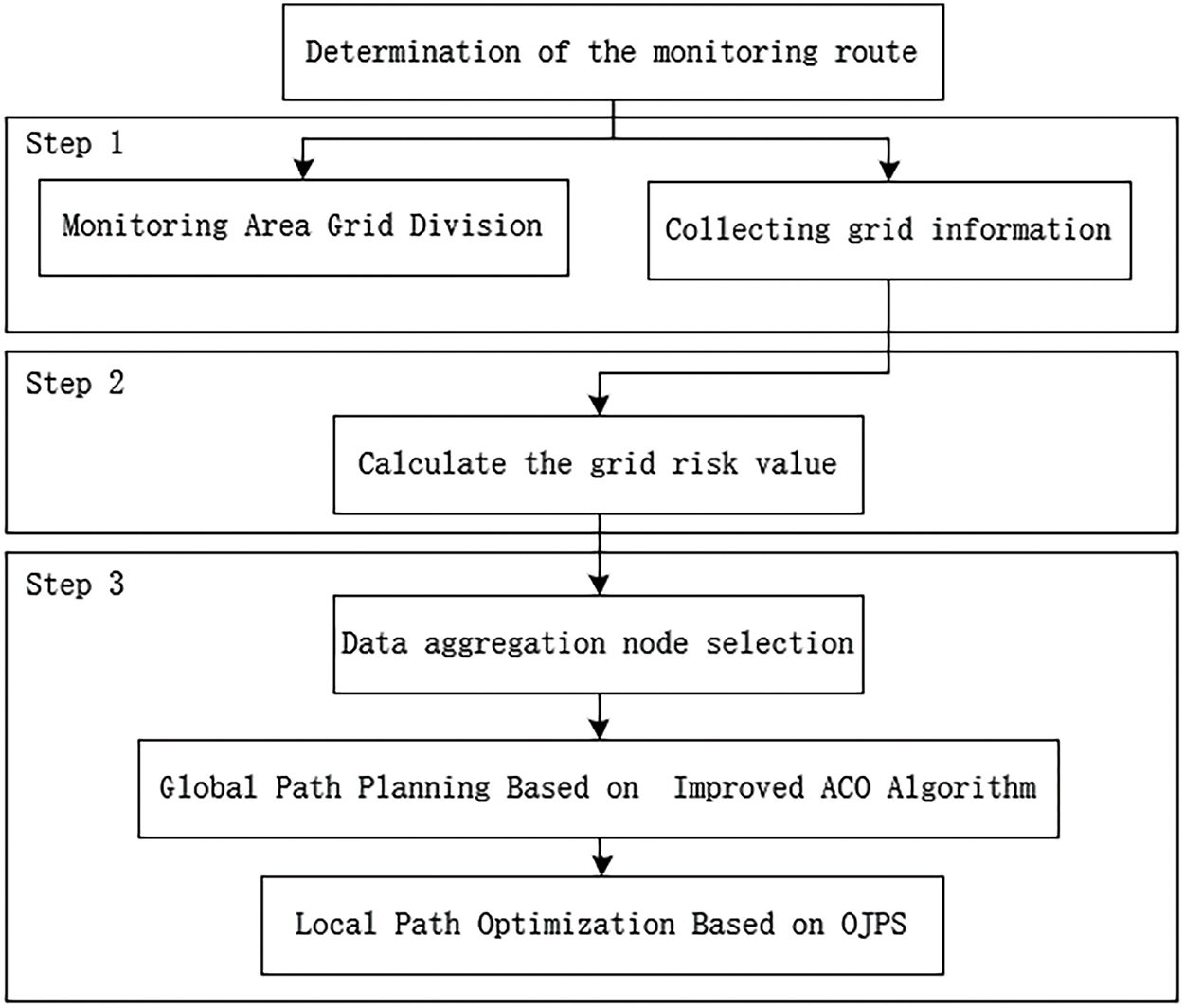
Figure 1: UAV monitoring path planning method

2.1 Environmental Event Gridding

In UAV path planning, the accurate two-dimensional modeling of the UAV’s motion environment constitutes a fundamental aspect of effective path planning. Commonly used modeling methods include the free space method, the grid method, and the topology method. After evaluating factors such as model complexity, validity, ease of implementation, and the clarity of obstacle representation, this paper adopts the grid method for modeling. Fig. 2 demonstrates an example of grid mapping, where the environment is divided into a series of grid cells, numbered sequentially from left to right and top to bottom. White grids indicate feasible regions, while black grids denote infeasible regions. Each grid cell is assigned specific positional coordinates, with the grid-coordinate relationship defined as follows:

{Xn={mod(n,N)−0.5,Xn≠−0.5N−0.5,Xn=−0.5Yn=ceil(nN)−0.5,(1)

where N denotes the number of grids per row, mod denotes the remainder operation, and ceil denotes the rounding operation.

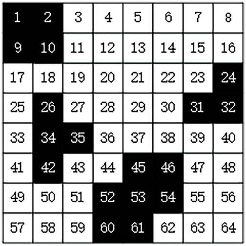
Figure 2: Schematic diagram of grid map

2.2 Data Aggregation Node Selection

In the process of constructing the grid map, each subdivided grid is defined as a node, and these nodes are the key units for data aggregation in monitoring path planning. The data aggregation nodes of monitoring paths need to be filtered based on the risk value of environmental events. The calculation of the risk value is a comprehensive assessment process, which is based on the number of environmental events inducing factors within each grid and the consequence severity of these inducing factors. The formula used to calculate the risk value is provided below:

R=∑i=1nωiDi,(2)

where R is the risk value of environmental events in the node area; n is the total number of inducing factors; ωi is the weight of the severity of the consequences of the i-th inducing factor; Di is the probability of occurrence of the i-th inducing factor. In order to ensure the comparability of the risk values, R is standardized so that it has a full score of 100, and a higher score indicates a higher risk of urban environmental events in the node region. The core of risk value calculation is to comprehensively evaluate the influence of multiple predisposing factors. Each inducing factor has a weight and an occurrence probability. The weight reflects the degree of influence of the inducing factors on the occurrence of environmental events, and the occurrence probability can reflect the extent of the potential risks in the area. Through the weighted sum of all inducing factors, the overall risk value R can be obtained so as to provide a decision basis for path planning. After completing the calculation of all grids corresponding to the corresponding risk value R, sorting from high to low is performed. Based on the sorting results, the top 5% of grids with the highest risk values are selected as data aggregation nodes for the UAV monitoring path.

2.3 Global Path Optimization with ACO Algorithm Based on Environmental Event Risk Value

2.3.1 Description of the Global Path Optimization Algorithm

The ACO algorithm is a metaheuristic algorithm inspired by the foraging behavior of ants. Its applications include a wide variety of optimization problems [26]. The core principle of the ACO algorithm is to emulate the collective behavior of ants in their search for food. Ants utilize pheromones for communication and guidance, which enables the gradual emergence of an optimal path.

In the field of urban environmental event monitoring, the application of ACO algorithms needs to be adapted to specific requirements. Traditional shortest path strategies are not always applicable to monitoring tasks, as the effectiveness of monitoring is often closely related to the environmental risk value of the path. To address this gap, this paper improves the ACO algorithm by introducing the environmental event risk value (R value) as a key factor in the algorithm’s decision-making process, so that the improved ant colony algorithm (R-ACO) comprehensively considers both the distance and the R value of the monitoring area when planning the path, in order to ensure that the planned paths cover the high-risk areas, to improve the effectiveness of the monitoring, and to achieve the objective of better data aggregation.

The traditional ACO algorithm sets the initial value of the pheromone as a constant, leading to the algorithm’s initial blind search and a significant reduction in search efficiency. The R-ACO algorithm incorporates the R value in the initial setting of the pheromone to enhance the accuracy of the initial search. The initial value of the pheromone is calculated according to the following equation:

τi,j(0)=k⋅Ridi,j+δ,(3)

where Ri is the R value of grid i, that is, the larger the R value is, the more valuable the region is to explore and the more ants tend to this region; k is a positive constant used to adjust the influence intensity of the R value; di,j is the distance from grid i to grid j; and δ is a very small positive number used to ensure numerical stability.

Furthermore, to further optimize the path selection so that the ants tend to explore an optimal path with monitoring value, R-ACO adapts the heuristic function to reduce the preference of the ants for nodes that are in close proximity but with low R-value during the search process. The improved heuristic function is defined by the following equation:

ηi,j(t)=Rjadi,j,(4)

where Rj is the risk value of the grid j to be transferred; a is a constant used to adjust the influence of R in the heuristic function.

In the pheromone updating strategy, the R-ACO algorithm considers the R value and length of the path to motivate the ants to explore the nodes with high R value and guide the ants to proceed in a more optimal direction. The improved pheromone update strategy is shown in the following equation:

τi,j(t+1)=ρ0⋅τi,j(t)+∑k=1mΔτi,jk(t),(5)

ρ0=(1−ρ)Rj,(6)

Δτi,jk(t)=RjLk,(7)

where Rj is the risk value of grid j to be transferred, ρ0 is the evaporation rate after considering the risk value; ∑k=1mΔτi,jk(t) is the pheromone left behind by all the ants in the current iteration iteration, and Lk is the path distance of ant k from grid i to grid j. This improved pheromone update strategy adds the consideration of R value on the basis of traditional information evaporation. The higher the R value of the path, the more pheromones the ants will leave, so as to guide the ants in the next iteration to explore this more, and finally form a positive feedback mechanism, which makes the algorithm realize effective monitoring in path planning. Ensure that high-risk areas receive more attention.

Finally, R-ACO uses the following state transfer probability formula to guide the ants in selecting the grid to be transferred next:

Pi,jk(t)={[τi,j(t)]α⋅[ηi,j(t)]β∑s∈allowedk[τi,s(t)]α⋅[ηi,s(t)]β,jϵallowedk0,j∉allowedk,(8)

where α and β denote the degree of influence of pheromone and distance on the ants’ path selection, respectively; allowedk is the set of grids to be transferred; τi,j(t) represents the pheromone concentration between the paths of grids i and j at the moment t; ηi,j(t) is the heuristic function.

2.3.2 Time Complexity Analysis of the R-ACO Algorithm

During the initialization phase of the R-ACO algorithm, an initial pheromone value is assigned to each grid node through a complete traversal of all nodes, resulting in a time complexity of O(N), where N denotes the total number of grid nodes. In the iterative phase, each ant evaluates and selects its next location at every step by traversing all feasible transition nodes. This operation exhibits an average time complexity of O(M) per ant per step, where M represents the average number of candidate nodes evaluated. After each iteration, a global pheromone update is performed across all grid nodes, contributing an additional O(N) complexity. Assuming the algorithm executes I iterations with A ants participating in each iteration, the overall time complexity of the improved ant colony algorithm is expressed as:

O(I⋅A⋅(N+M)).(9)

2.3.3 Space Complexity Analysis of the R-ACO Algorithm

The spatial complexity of the R-ACO algorithm is primarily driven by three key components: the pheromone matrix, ant position tracking, and the candidate node set during state transitions. The pheromone matrix, which stores pheromone values for all N grid nodes, requires O(N2) space. Additionally, maintaining the current positions of A ants occupies O(A) space. During state transitions, the algorithm must temporarily store feasible candidate nodes, and in the worst-case scenario where all N nodes are considered, this operation contributes O(N) space. Therefore, the total spatial complexity of the R-ACO algorithm is expressed as:

O(N2+A+N).(10)

2.4 Local Path Optimization Based on the OJPS Algorithm

2.4.1 Description of the OJPS Algorithm

In the complex background of an urban environment, UAVs performing global path planning tasks often encounter localized dead zones caused by the dense distribution of obstacles, which may trigger the algorithm’s deadlock state [27]. To overcome this issue, this paper proposes an innovative local path optimization strategy, termed the OJPS algorithm.

The OJPS algorithm is a derived version of the Jump Point Search (JPS) algorithm [28], which in itself is an improvement on the A* algorithm. The JPS algorithm markedly enhances the efficiency of path search by identifying and retaining the pivotal nodes (i.e., jump points) in the path search while discarding the non-critical nodes. This approach not only optimizes the search process but also maintains the accuracy of path planning. The core innovation of the OJPS algorithm is its further simplification of the search space. The algorithm considers only orthogonal (i.e., horizontal and vertical) movements in the grid map and excludes the search in the diagonal direction, as shown in Fig. 3, which shows the flowchart of the OJPS algorithm. This strategy is based on the observation that obstacles in urban environments are usually arranged in an orthogonal grid, which reduces the number of nodes that need to be evaluated during the search process, thereby enhancing the efficiency of the algorithm and the accuracy of path planning.

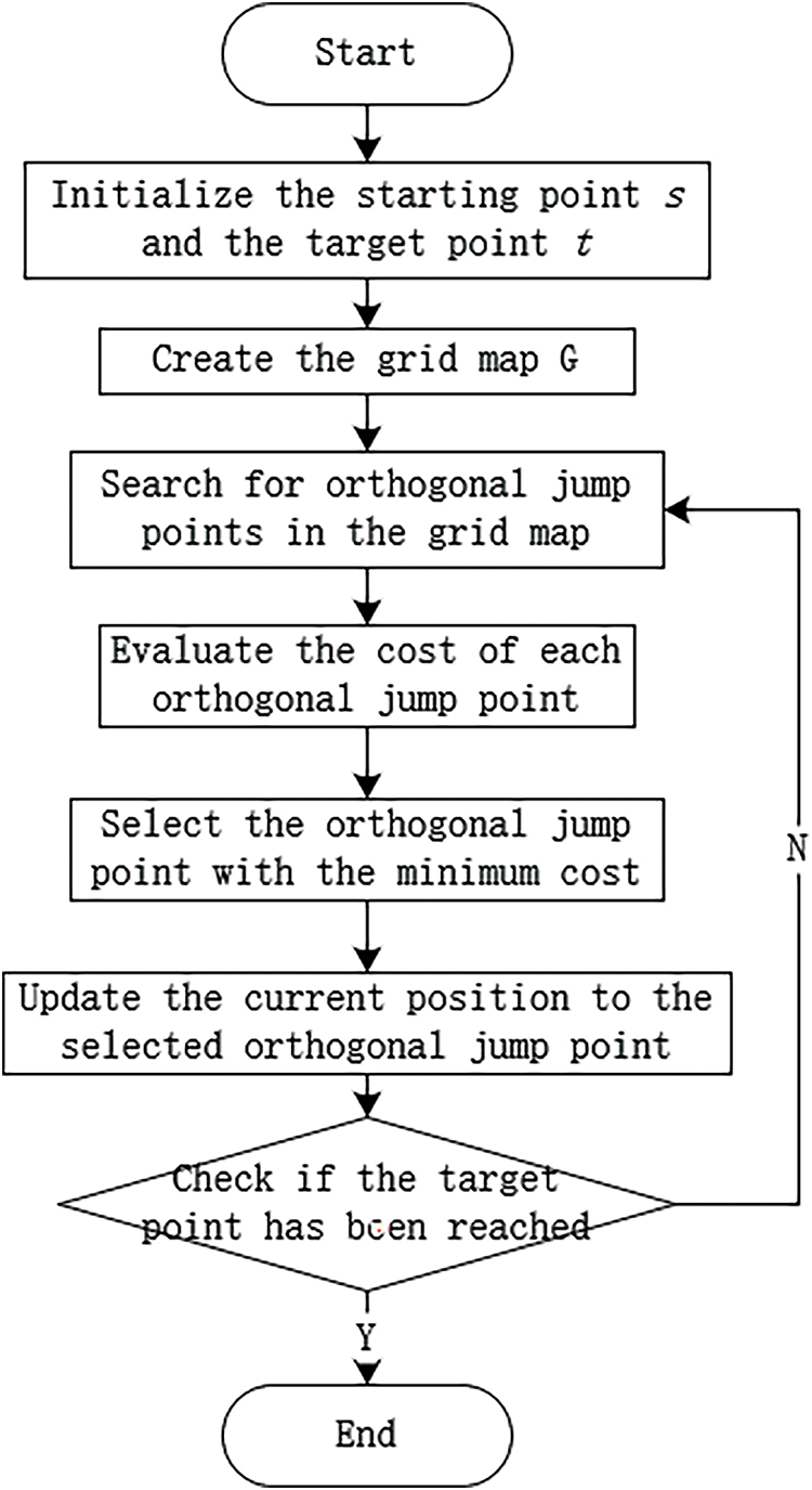
Figure 3: Flowchart of OJPS algorithm

With this orthogonal direction search strategy, the OJPS algorithm is able to effectively avoid local dead zones and provide a clearer path planning scheme for UAVs. In addition, the simplified search space characteristic of the OJPS algorithm makes it scalable and adaptable while maintaining high efficiency, which is suitable for a variety of complex urban environmental event monitoring tasks.

In the OJPS algorithm, an orthogonal jump point is defined as a move from the current position to the next reachable position along an orthogonal direction, that is, only along the horizontal or vertical axes. The screening of orthogonal jump points represents the core of the OJPS algorithm, as it determines the accuracy of node selection during the search process. In the grid map G, each grid is considered as a node, and the eight grids adjacent to the current node are called the set of nodes “around the current node”. Let the current node position be the parent node P(x), and the next node to be moved to is x. The jump-point filtering mechanism can be divided into two cases: one is when there is no obstacle around the current node, and the other is when there is an obstacle.

2.4.2 No Obstacles around the Current Node

As shown in Fig. 4, when searching upward from point P(x) in an obstacle-free environment, the path through node x to reach the next node n (e.g., from node 7 through node 4 to reach node 1) is deemed to be a valid jumping point if it is shorter than the path without x to reach node n (e.g., by jumping from node 7 directly to node 1) directly from P(x). In this case, the gray nodes (2, 3, 5, 6, 8, 9) are considered invalid nodes, and they do not participate in the calculation of the path length; they are defined as invalid nodes. Therefore, the filtering condition can be expressed as:

L(P(x),⋅⋅⋅,n/x)≥L(P(x),x,n),(11)

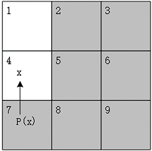
Figure 4: Schematic diagram of search without obstacles around the node

where L() denotes the path length, [P(x),…,n/x] is the path from P(x) to n without passing through x; [P(x),x,n] is the path P(x) passing through x to n. n is the movable nodes around node x.

2.4.3 Obstacles around the Current Node

As shown in Fig. 5, when there is an obstacle node around node x (node 2 in Fig. 5), the screening method in the case of no obstacle is inapplicable, necessitating the adoption of an alternative screening rule. In this case, a node n is said to be a forced neighbor of node x if the path through node x to the next node n (from node 7 through node 4 to node 2 in Fig. 5) is shorter than the path directly to node n without nodes (from node 7 to node 2 in Fig. 5), and node n is not a natural neighbor of node x. MN in Fig. 5 is the required neighbor point. The mandatory neighbors are filtered as follows:

n∉NaturalNeighbors(x),(12)

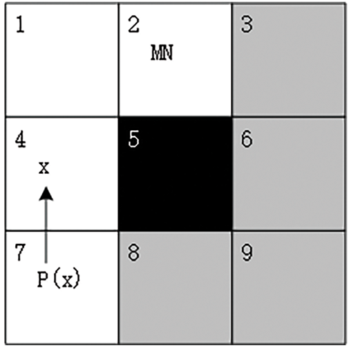
Figure 5: Schematic diagram of search with obstacles around the node

and:

L(P(x),⋅⋅⋅,n/x)>L(P(x),x,n),(13)

where NaturalNeighbors(x) denotes the set of natural neighbors of node x.

Through the screening of these two cases, the OJPS algorithm can effectively identify the critical jump points, thus optimizing the path search process and improving the efficiency of the algorithm and the quality of path planning.

When the screening of orthogonal jump points is completed, the obtained orthogonal jump points will be added to the Openlist table of the A* algorithm for evaluation, and the evaluation function is shown in Eq. (14):

f(n)=h(n)+g(n),(14)

where f(n) is the evaluation function, h(n) is the path cost from the current node to the target node and g(n) is the path cost from the start node to the current node. The target node with the smallest surrogate value is selected and added to the Closer list table of the A* algorithm, and then the paths are obtained by connecting the nodes in the Closer list table. The A* algorithm can only select the neighboring 8 directions in the next node selection for the computation, whereas the OJPS algorithm selects from the orthogonal jumping points, which allows the algorithm to perform a long-distance move across multiple nodes. This long-range and restricted orthogonal direction jump selection mechanism significantly improves the operational efficiency of the path search while maintaining the accuracy of the path planning. This feature of the OJPS algorithm makes it particularly suitable for local path optimization of UAVs in urban environmental event monitoring, where fast response and efficient path optimization delineation are crucial for the success of the monitoring mission.

2.4.4 Time Complexity Analysis of the OJPS Algorithm

The core mechanism of the OJPS algorithm lies in its effective identification of orthogonal jump points. This process systematically examines the neighborhood of each node to determine eligible jump points. For any given node, the algorithm evaluates up to four neighboring nodes, with this number reaching its maximum in obstacle-free environments or increasing adaptively in the presence of obstacles. Since this process primarily involves a fixed number of comparison and calculation operations, its time complexity is classified as O(1) (constant time complexity). During the path search phase, the OJPS algorithm adopts the A* algorithm framework while optimizing the Openlist update strategy through orthogonal jump point recognition. Although extreme cases may require revisiting most graph nodes, the ability to filter non-critical nodes via jump point identification significantly reduces the number of evaluated nodes. Let V denote the total number of nodes in the graph, and V′ represent the actual number of nodes evaluated by OJPS. Empirically, V′ is often less than V. Thus, the overall time complexity of the OJPS algorithm is expressed as:

O(V′).

2.4.5 Space Complexity Analysis of the OJPS Algorithm

The OJPS algorithm relies on two critical data structures: the Openlist and Closelist. The Openlist temporarily stores unevaluated nodes, whereas the Closelist records evaluated nodes. In the worst-case scenario, where all nodes require evaluation, both lists must store the entire set of V nodes, resulting in a space complexity of O(V) for each list. Considering the storage demands of these data structures and auxiliary information for orthogonal jump points, the total spatial complexity of the OJPS algorithm remains: O(V).

3  Numerical Experiments and Analysis of Results

3.1 Experimental Setup

In order to verify the feasibility and superiority of the R-ACO and OJPS algorithms proposed in this paper in UAV path optimization, numerical experiments are conducted through MATLAB. The UAV model is set to fly at a speed of 1 m/s, and each turning time is set to 4 s. The experimental setup includes:

Global path planning: The classic solution strategy of the traveling salesman problem is adopted, the eil51 standard data set is used, and the corresponding risk value is attached to each coordinate. The average risk value of the R-ACO algorithm, PSO algorithm, and ARO algorithm under different time scales of parameters is compared.

Local Path Optimization: Comparing the performance of the OJPS algorithm with other path planning algorithms in terms of path duration and number of turns in a 2D grid model of a simulated urban environment, using the Manhattan distance as a heuristic function.

3.2 Experimental Results and Analysis

3.2.1 Comparison of Global Path Planning Experiment Results

Fig. 6 shows the path planning results of the three algorithms, where the green node is the starting position, the number labeled next to each node indicates the risk value of the environmental event at that node, and the direction of the path is indicated by the direction of the arrow. In Fig. 6a, the path length planned by the R-ACO algorithm is 671.9681 m; in Fig. 6b, the path length planned by the PSO algorithm is 1308.6833 m; in Fig. 6c, the path length planned by the ARO algorithm is 1336.0146 m. By comparing the path planning graphs of the three algorithms, it can be observed that there is a significant difference between the PSO algorithm and the ARO algorithm in the global path planning using the strategy of solving the TPS problem and the R-ACO algorithm. The optimal path length planned by the two algorithms is still larger than that of the R-ACO algorithm without considering the environmental risk value. The R-ACO algorithm shows a trade-off between risk value and distance in path planning, which ensures effective data aggregation for key nodes with high R value.

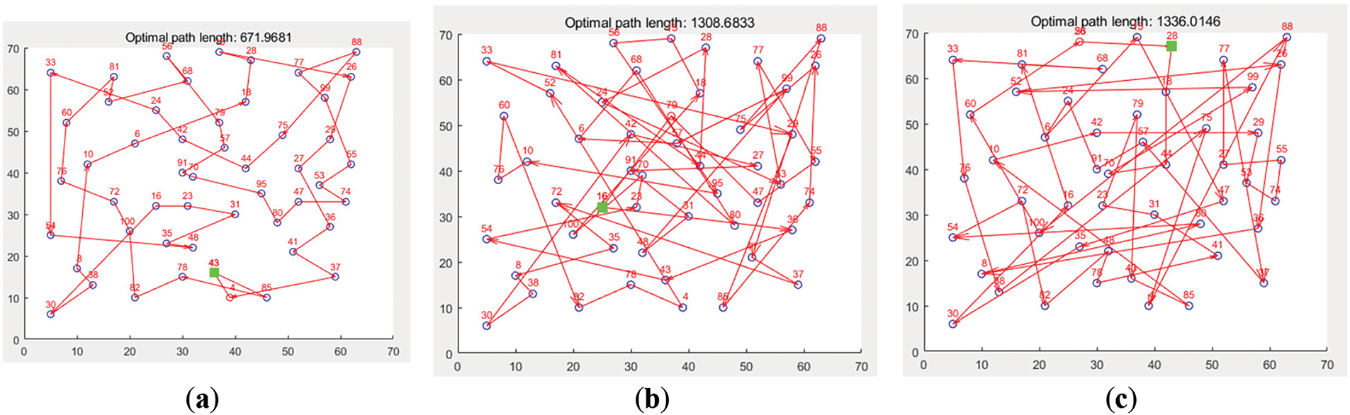
Figure 6: Path planning results of the different algorithms. (a) R-ACO algorithm path planning diagram; (b) PSO algorithm path planning diagram; (c) ARO algorithm path planning diagram

Fig. 7 shows the average R value of the path node traversed by the three algorithms at different times. In the figure, I is the average R value of the path node traversed within 5 min, II is the average R value of the path node traversed within 8 min, and III is the average R value of the path node traversed within 10 min. Within 5 min, the average R value of the path nodes of the R-ACO algorithm is 71.21, which is 48.33% and 70.33% higher than that of the PSO algorithm and ARO algorithm, respectively. Within 8 min, the average R value of path nodes is 59.87, which is 26.10% and 19.08% higher than that of the PSO algorithm and ARO algorithm, respectively. Within 10 min, the average R value of path nodes is 53.79, which is 6.746% and 10.246% higher than that of the PSO algorithm and ARO algorithm, respectively. Although the average R value of the path traversed by R-ACO algorithm in the first 8 and 10 min is lower than that in the first 5 min, and the improvement degree is also lower than that of PSO algorithm and ARO algorithm, this is because R-ACO algorithm is close to the end of path planning at 8 and 10 min. The PSO algorithm and ARO algorithm are in the middle stage of exploration, and the R-ACO algorithm at this time explores more areas with low R value so that the final average R value is reduced. However, in general, the R-ACO algorithm still performs better than the PSO algorithm and ARO algorithm in the average R value of the path traversed in three time nodes, which shows that the R-ACO algorithm can comprehensively consider the R value and the distance in the search process, to carry out more reasonable path planning. Therefore, the proposed algorithm has higher practical application value in UAV path planning for urban environmental event monitoring.

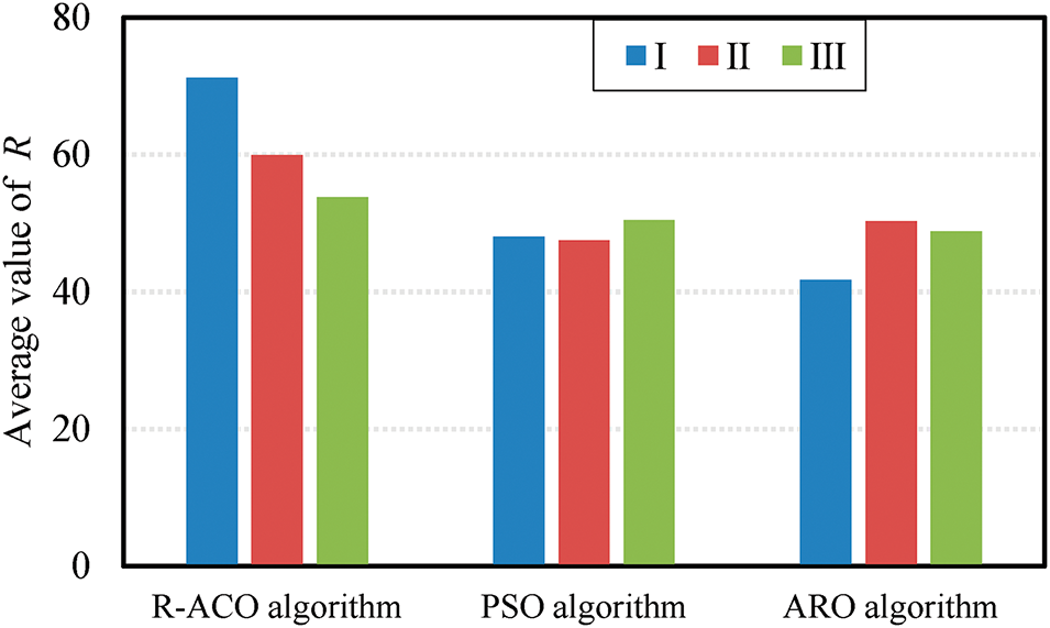
Figure 7: Value of R in different methods

3.2.2 Comparison of Experimental Results for Local Path Optimization

Fig. 8 shows the experimental path results of the four algorithms in the two-dimensional grid model simulating the same complex urban environment, where the heuristic function of the A* algorithm, JPS algorithm, and OJPS algorithm is to choose Manhattan distance, which is more conducive to the comparison of results. In the figure, the green grid is the starting position, the red grid is the end position, the gray grid is the obstacle, and the white grid is the feasible region. Fig. 8a shows the path result of the Dijkstra algorithm, and the path length is 58 m. Fig. 8b shows the path result of the A* algorithm, and the path length is 58 m. Fig. 8c shows the path result of the JPS algorithm, and the path length is 45.7 m. Fig. 8d shows the path result of the OJPS algorithm with a path length of 58 m. Fig. 8 shows that although the OJPS algorithm has no obvious advantage in path length, its path is more concise and direct and has a better search range, which can improve the search efficiency in practical applications.

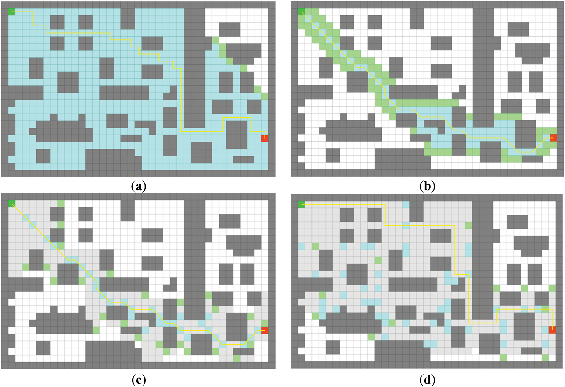
Figure 8: The stimulation of path planning results in different ways. (a) Dijkstra algorithm; (b) A* algorithm; (c) JPS algorithm; (d) OJPS algorithm

Fig. 9 comprehensively shows the performance of the four algorithms in terms of the number of path turns and the total flight duration, where I is the number of turns and II is the total flight duration. The OJPS algorithm is significantly better than the other algorithms in the number of turns with only 9, which is 40%, 40%, and 57.1% less compared to the JPS algorithm, the A* algorithm, and the Dijkstra algorithm, respectively. Considering that the ability to turn the Angle of a UAV is limited by dynamic and environmental factors, reducing the number of turning angles can not only improve the flight stability of UAV but also improve its monitoring efficiency. The OJPS algorithm effectively reduces the number of nodes that need to be considered by restricting the search direction of jumping points to the orthogonal direction and thus performs well in terms of the number of turning times, which is especially important for UAVs to perform the task of monitoring urban environmental events. In terms of total flight time, the OJPS algorithm completes the flight in 94 s, which is 11.1%, 11%, and 33.8% shorter than the JPS algorithm, the A* algorithm, and the Dijkstra algorithm, respectively. The result is due to the optimization of the OJPS algorithm in terms of the number of turns, which also significantly reduces the flight time. This is crucial for responding to urgent urban environmental events, enabling the UAV to respond quickly and complete the monitoring task in time.

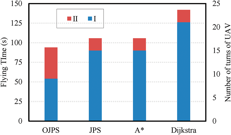
Figure 9: Flying time and number of turns of UAV in different methods

In summary, the advantages of the OJPS algorithm in reducing the number of turns and flight time demonstrate high efficiency and effectiveness in monitoring urban environmental events. These properties make the OJPS algorithm ideal for rapid local optimization in UAV path planning, helping to facilitate the successful completion of monitoring tasks.

3.3 Sensitivity Analysis of Key Parameters of R-ACO Algorithm

To further explore the effects of different parameters on the performance of the proposed R-ACO algorithm, we conduct a sensitivity analysis. By systematically changing the number of ants, the pheromone influence degree factor, and the power of R value, and the change of path length is also observed when other conditions remain unchanged, the specific effects of these parameters on the performance of the algorithm can be evaluated.

Table 1 shows how the path length varies with different parameter combinations. As shown in Table 1, the number of ants has a relatively minor effect on the path length, with an increase in the number of ants leading to a slight reduction in path length. In contrast, the pheromone influence degree factor and the power of R value have more pronounced impacts. Specifically, increasing the pheromone influence degree factor from 2 to 3 significantly decreases the path length, whereas reducing it to 1 leads to a substantial increase. Most notably, the power of R value exhibits the most significant influence on the path length, with its increase from 3 to 4 resulting in a dramatic rise in the path length.

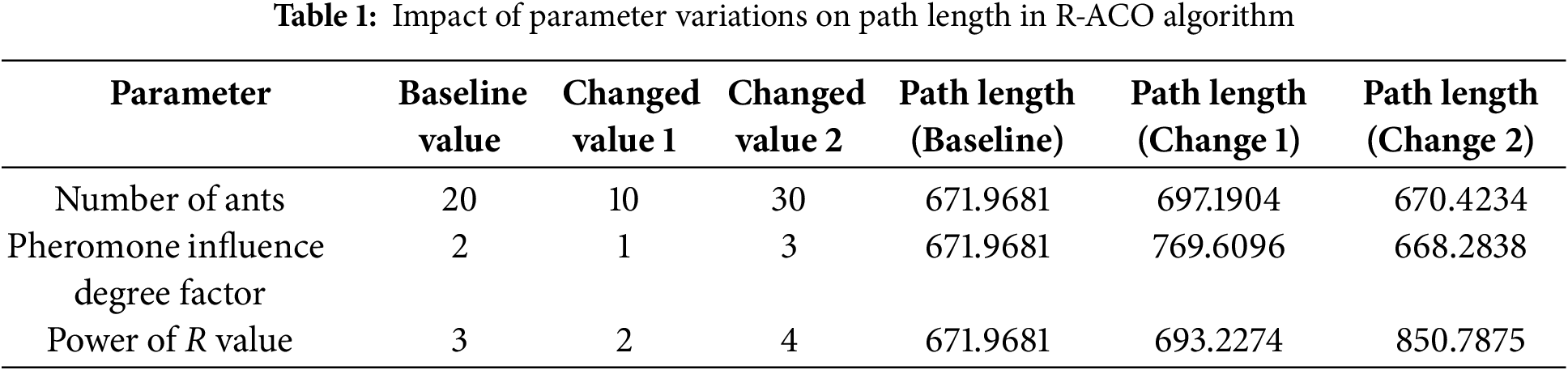
In summary, sensitivity analysis showed that the pheromone influence degree factor and the power of R has the most significant effect on the path length, especially the power of R. These findings provide an important reference for optimizing algorithm parameters and lay a foundation for further research.

4  Simulation Experiment

At the end of the simulation experiment, an actual path experiment will be conducted. In the experiments, a 20 × 20 grid map with distributed obstacles is designed in this paper for simulating the real situation. The black areas in the map indicate obstacles, the white areas indicate feasible regions, and the grid of each feasible region is labeled with the corresponding R value. In this experiment, the R-ACO algorithm and the traditional ACO algorithm are used for path planning on the same grid map, and the starting point and the end point of the experiment are set as Grid 1 and Grid 400, respectively. A comparison graph of the experimental results is shown in Fig. 10.

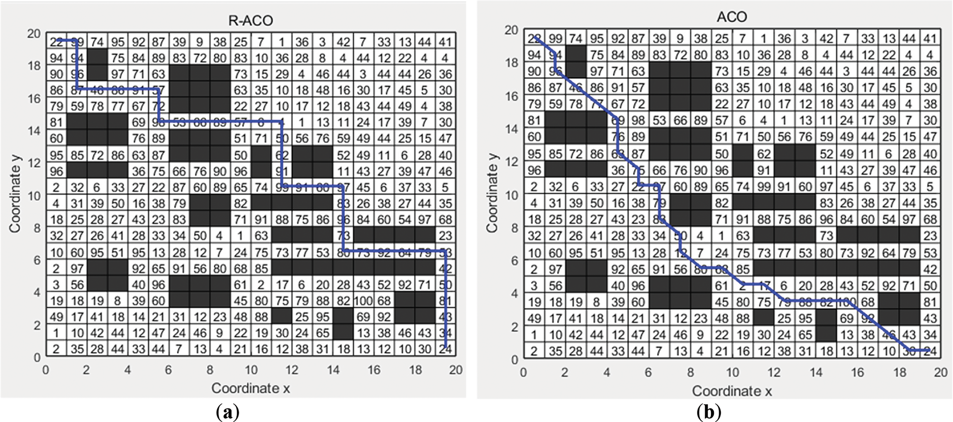
Figure 10: Path planning results of the R-ACO and ACO algorithms. (a) R-ACO algorithm; (b) ACO algorithm

Fig. 10a shows the path planned by the R-ACO algorithm and Fig. 10b shows the path planned by the ACO algorithm, from the figure it can be seen that the path planned by the ACO algorithm suffers from a high number of turns and a complex path, while the R-ACO algorithm, due to the adoption of the OJPS algorithm in the local planning, makes the planned path have the advantage of simplicity and clarity and a low number of turns.

Fig. 11 shows the comparison between the R-ACO algorithm and the ACO algorithm in terms of path average R value, path length, and number of turns, where I is the path average R value, II is the path length, and III is the number of turns. The path average R-value and the number of turns for the R-ACO algorithm are 67.79 and 9, respectively, which is an increase of 9.55% and 47.06% in the two performance indexes compared with the ACO algorithm, respectively. This is due to the fact that the R-ACO algorithm considers the R value during path planning and utilizes the OJPS algorithm for local path planning, which enables the UAV to plan a monitoring-valued path when performing environmental event monitoring tasks, and at the same time effectively reduces the number of turning times in order to improve flight efficiency when encountering complex obstacles. As for the path length, although the R-ACO algorithm plans a path length of 38 m, which is slightly inferior to the 34.97 m planned by the ACO algorithm, this path gap is obviously acceptable considering that the R-ACO algorithm is a combination of the R value as well as the distance for the path search.

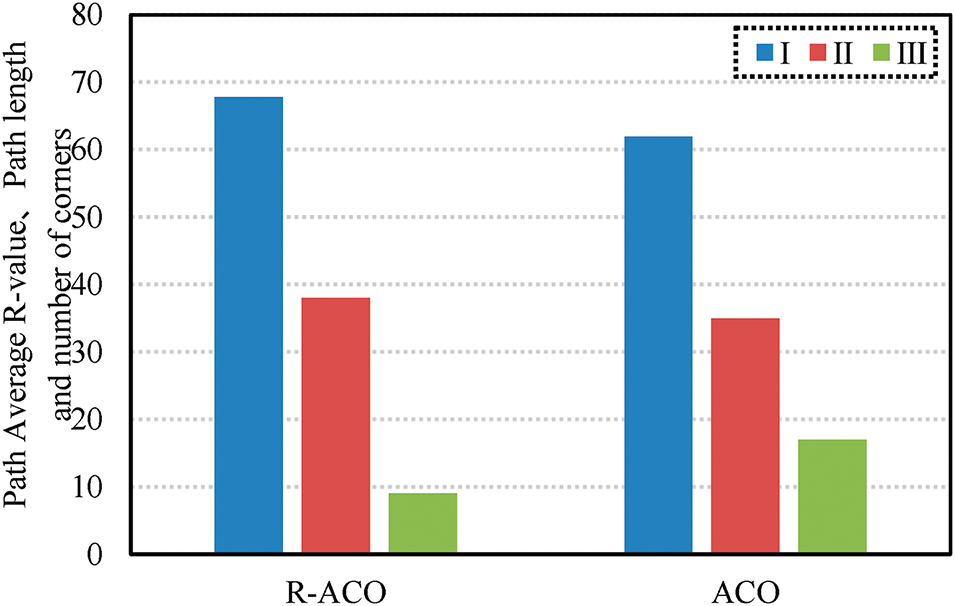
Figure 11: Path-averaged R-value, path length, and number of turns for R-ACO and ACO algorithms

Furthermore, experiments were conducted on path planning in a 3D environment, as illustrated in Fig. 12. The experiment utilizes a 5 × 5 × 5 3D rasterized map to depict the urban environment, wherein the grid points represent the monitoring points present in the 3D environment, and the colors of the different grid points indicate the R values of the environmental events, with a color gradient from blue (low risk) to red (high risk). The black connecting line indicates the flight path generated by the UAV according to the optimized path planning algorithm. The green star symbolizes the initial point, while the blue square denotes the terminal point.

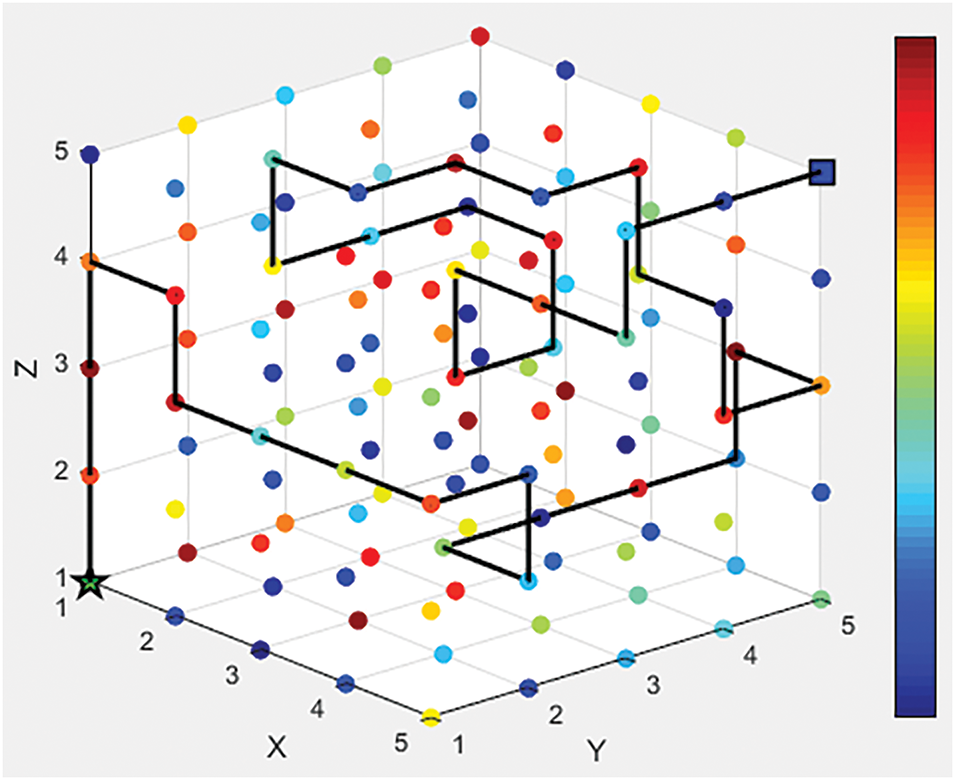
Figure 12: Path planning results in 3D environment

As illustrated in Fig. 12, the path planning method proposed in this paper prioritizes the exploration of monitoring points with high R-values in urban environments. Additionally, searching along orthogonal directions can minimize excessive cornering when the UAV performs the monitoring task. This can assist the UAV in effectively reducing energy loss due to excessive cornering during flight. In summary, the UAV path planning method for environmental event monitoring proposed in this paper is effective.

5  Conclusion

This paper presents an innovative UAV path-planning method that incorporates the OJPS algorithm and the R-ACO algorithm. After reviewing the blindness of the traditional ACO algorithm in the initial search phase and the limitations of its applicability in urban environmental event monitoring, this paper introduces the concept of R value to critically improve the ACO algorithm. This improvement significantly enhances the relevance and effectiveness of path planning, ensuring that the generated paths not only consider the R value but also synthesize the distance factor between grids, thus providing a path with practical monitoring significance for UAVs in urban environmental event monitoring. Aiming at the common vertical or horizontal obstacles in the urban environment, the OJPS algorithm proposed in this paper effectively solves the path planning difficulties caused by local complex obstacles by restricting the search direction to orthogonal directions. Both numerical experiments and practical application cases fully prove the effectiveness and superiority of the method.

Although the path planning method proposed in this paper shows a broad application prospect, there are still some aspects that need to be further explored.

(1)   UAV Battery Capacity: The current method does not explicitly account for UAV battery constraints. In real-world applications, battery capacity directly impacts flight duration and mission success. Future work should explore strategies to optimize path planning while considering energy consumption.

(2)   Communication Range: Effective communication between UAVs and ground stations is crucial for successful missions. Our method assumes reliable communication; however, varying communication ranges can affect task coordination. The study of adaptive communication protocols will be an effective means of improving the reliability of operations in the future.

(3)   Environmental Variables: Environmental factors, such as weather conditions (e.g., wind, precipitation), can significantly influence UAV performance. Incorporating dynamic environmental variables into the path planning process is an important future research direction to improve the robustness of algorithms in different and unpredictable environments.

Acknowledgement: Not applicable.

Funding Statement: The work is supported by the Special Project for Key Fields of Ordinary Universities in Guangdong Province (Number: 2023ZDZX1076).

Author Contributions: The authors confirm contribution to the paper as follows: study conception and design: Huiru Cao, Yongxin Liu; data collection: Shaoxin Li; analysis and interpretation of results: Shaoxin Li; draft manuscript preparation: Xiaomin Li. All authors reviewed the results and approved the final version of the manuscript.

Availability of Data and Materials: The readers can access the data used in the study by contacting the corresponding author.

Ethics Approval: Not applicable.

Conflicts of Interest: The authors declare no conflicts of interest to report regarding the present study.

References

1. Peduzzi P. The disaster risk, global change, and sustainability nexus. Sustainability. 2019;11(4):957. doi:10.3390/su11040957. [Google Scholar] [CrossRef]

2. Satir O, Kemec S, Yeler O, Akin A, Bostan P, Mirici ME. Simulating the impact of natural disasters on urban development in a sample of earthquake. Nat Hazards. 2023;116(3):3839–55. doi:10.1007/s11069-023-05838-w. [Google Scholar] [CrossRef]

3. Outay F, Mengash HA, Adnan M. Applications of unmanned aerial vehicle (UAV) in road safety, traffic and highway infrastructure management: recent advances and challenges. Transp Res Part A Policy Pract. 2020;141:116–29. doi:10.1016/j.tra.2020.09.018. [Google Scholar] [PubMed] [CrossRef]

4. Wang Z, Chen J, Cheng W, Arulrajah A, Horpibulsuk S. Investigation into the tempo-spatial distribution of recent fire hazards in China. Nat Hazards. 2018;92:1889–907. doi:10.1007/s11069-018-3264-5. [Google Scholar] [CrossRef]

5. Fu G, Wang J, Yan M. Anatomy of tianjin port fire and explosion: process and causes. Process Saf Prog. 2016;35(3):216–20. doi:10.1002/prs.11837. [Google Scholar] [CrossRef]

6. Stöcker C, Bennett R, Nex F, Gerke M, Zevenbergen J. Review of the current state of UAV regulations. Remote Sens. 2017;9(5):459. doi:10.3390/rs9050459. [Google Scholar] [CrossRef]

7. Manfreda S, McCabe MF, Miller PE, Lucas R, Pajuelo Madrigal V, Mallinis G, et al. On the use of unmanned aerial systems for environmental monitoring. Remote Sens. 2018;10(4):641. doi:10.3390/rs10040641. [Google Scholar] [CrossRef]

8. Zhang Y, Yuan X, Li W, Chen S. Automatic power line inspection using UAV images. Remote Sens. 2017;9(8):824. doi:10.3390/rs9080824. [Google Scholar] [CrossRef]

9. Dong J, Ota K, Dong M. UAV-based real-time survivor detection system in post-disaster search and rescue operations. IEEE J Miniaturization Air Space Syst. 2021;2(4):209–19. doi:10.1109/JMASS.2021.3083659. [Google Scholar] [CrossRef]

10. Yang Z, Yu X, Dedman S, Rosso M, Zhu J, Yang J, et al. UAV remote sensing applications in marine monitoring: knowledge visualization and review. Sci Total Environ. 2022;838:155939. doi:10.1016/j.scitotenv.2022.155939. [Google Scholar] [PubMed] [CrossRef]

11. Asadzadeh S, de Oliveira WJ, de Souza Filho RC. UAV-based remote sensing for the petroleum industry and environmental monitoring: state-of-the-art and perspectives. J Pet Sci Eng. 2022;208(11):109633. doi:10.1016/j.petrol.2021.109633. [Google Scholar] [CrossRef]

12. Sudhakar S, Vijayakumar V, Kumar CS, Priya V, Ravi L, Subramaniyaswamy V. Unmanned aerial vehicle (UAV) based forest fire detection and monitoring for reducing false alarms in forest-fires. Comput Commun. 2020;149(7):1–16. doi:10.1016/j.comcom.2019.10.007. [Google Scholar] [CrossRef]

13. Xiao Y, Guo Y, Yin G, Zhang X, Shi Y, Hao F, et al. UAV multispectral image-based urban river water quality monitoring using stacked ensemble machine learning algorithms—a case study of the Zhanghe River. China Remote Sens. 2022;14(14):3272. doi:10.3390/rs14143272. [Google Scholar] [CrossRef]

14. Bortoff SA. Path planning for UAVs. In: Proceedings of the 2000 American Control Conference. ACC (IEEE Cat. No. 00CH36334); 2000 Jun 28–30; Chicago, IL, USA. p. 364–8. [Google Scholar]

15. Dijkstra EW. A note on two problems in connexion with graphs. Numer Math. 1959;1(1):269–71. doi:10.1007/BF01386390. [Google Scholar] [CrossRef]

16. Hart PE, Nilsson NJ, Raphael B. A formal basis for the heuristic determination of minimum cost paths. IEEE Trans Syst Sci Cybern. 1968;4(2):100–7. doi:10.1109/TSSC.1968.300136. [Google Scholar] [CrossRef]

17. Lavalle S. Rapidly-exploring random trees: a new tool for path planning. In: Research report 9811. Ames, IA, USA: Department of Computer Science, Iowa State University; 1998. [Google Scholar]

18. Liu C, Wu L, Li G, Zhang H, Xiao W, Xu D, et al. Improved multi-search strategy A* algorithm to solve three-dimensional pipe routing design. Expert Syst Appl. 2024;240(1):122313. doi:10.1016/j.eswa.2023.122313. [Google Scholar] [CrossRef]

19. Holand JH. Adaptation in natural and artificial systems. Vol. 32. Ann Arbor, MI, USA: The University of Michigan Press; 1975. [Google Scholar]

20. Kennedy J, Eberhart R. Particle swarm optimization. In: Proceedings of ICNN’95—International Conference on Neural Networks; 1995 Nov 27–Dec 1; Perth, WA, Australia. p. 1942–8. [Google Scholar]

21. Colorni A, Dorigo M, Maniezzo V, Trubian M. Ant system for job-shop scheduling. Jorbel-Belg J Oper Res Stat Comput Sci. 1994;34(1):39–53. [Google Scholar]

22. Xu N, Zhu H, Sun J. Bionic 3D path planning for plant protection UAVs based on swarm intelligence algorithms and krill swarm behavior. Biomimetics. 2024;9(6):353. doi:10.3390/biomimetics9060353. [Google Scholar] [PubMed] [CrossRef]

23. Garip Z, Karayel D, Erhan çimen M. A study on path planning optimization of mobile robots based on hybrid algorithm. Concurr Comput Pract Exp. 2022;34(5):e6721. doi:10.1002/cpe.6721. [Google Scholar] [CrossRef]

24. Bai X, Jiang H, Cui J, Lu K, Chen P, Zhang M. UAV path planning based on improved A* and dwa algorithms. Int J Aerosp Eng. 2021;2021(1):4511252. doi:10.1155/2021/4511252. [Google Scholar] [CrossRef]

25. Hu Z, Chen H, Lyons E, Solak S, Zink M. Towards sustainable UAV operations: balancing economic optimization with environmental and social considerations in path planning. Transp Res Part E Logist Transp Rev. 2024;181(18):103314. doi:10.1016/j.tre.2023.103314. [Google Scholar] [CrossRef]

26. Blum C. Ant colony optimization: introduction and recent trends. Phys Life Rev. 2005;2(4):353–73. doi:10.1016/j.plrev.2005.10.001. [Google Scholar] [CrossRef]

27. Isloor SS, Marsland TA. The deadlock problem: an overview. Computer. 1980;13(9):58–78. doi:10.1109/MC.1980.1653786. [Google Scholar] [CrossRef]

28. Harabor D, Grastien A. Online graph pruning for pathfinding on grid maps. In: Proceedings of the AAAI Conference on Artificial Intelligence; 2011 Aug 7–11; San Francisco, CA, USA. p. 1114–9. [Google Scholar]